Article

Interactions Obtained from Basic Mechanistic Principles: Prey Herds and Predators

by
Cecilia Berardo
1,*,
Iulia Martina Bulai
2,3 and
Ezio Venturino
3,4
1
Department of Mathematics and Statistics, University of Helsinki, FI-00014 Helsinki, Finland
2
Department of Mathematics, Informatics and Economics, University of Basilicata, I-85100 Potenza, Italy
3
GNCS Research Group, INdAM, I-00185 Rome, Italy
4
Department of Mathematics Giuseppe Peano, University of Torino, I-10100 Torino, Italy
*
Author to whom correspondence should be addressed.
Mathematics 2021, 9(20), 2555; https://doi.org/10.3390/math9202555
Submission received: 31 August 2021 / Revised: 21 September 2021 / Accepted: 1 October 2021 / Published: 12 October 2021

Abstract

:
We investigate four predator–prey Rosenzweig–MacArthur models in which the prey exhibit herd behaviour and only the individuals on the edge of the herd are subjected to the predators’ attacks. The key concept is the herding index, i.e., the parameter defining the characteristic shape of the herd. We derive the population equations from the individual state transitions using the mechanistic approach and time scale separation method. We consider one predator and one prey species, linear and hyperbolic responses and the occurrence of predators’ intraspecific competition. For all models, we study the equilibria and their stability and we give the bifurcation analysis. We use standard numerical methods and the software Xppaut to obtain the one-parameter and two-parameter bifurcation diagrams.

1. Introduction

Modelling herd behaviour of a population with ordinary differential equations, via a spatial factor with herding index (see Laurie et al. [1]), avoids an explicit spatial representation.
Already in 1987, Liu and colleagues [2] used the herding index, represented by an exponent, to give a non-linear incidence rate in epidemiological models, and later this concept found several applications in the same context [3,4].
The herding index, α in this article, also appeared in predator–prey dynamics with prey grouped in herd. In particular, the first studies comprised only the case α = 1 / 2 by assuming a two-dimensional herd representation [5,6], while later works allowed for a fixed herding index in the range [ 1 / 2 , 1 ) [6,7]. The concept of herding index was further extended to models other than ordinary differential equations, such as time delay equations, [8], and fractional differential equations [9,10].
In predator–prey models, the assumption that the prey gather in a herd has a direct effect on the shape of the functional response, as the encounter rate of the predator and prey individuals increases with the prey density according to the herding index. Therefore, in the simple case of no prey handling, we obtain the herd-linear functional response. More complex is the herd-Holling type II functional response, already used by Djilali in [8] in a time delay differential model, which we derive in this paper from a system of fast time-scale state transitions.
The mechanistic derivation of the functional response follows from the time-scale separation method that has been recently formalised by Berardo et al. [11] and previously used in the works by Geritz and Gyllenberg [12,13,14]. In particular, analogously to Metz and Diekmann [15], we assume the predators in two states, searching and handling, and model the state transitions on a fast time-scale compared to other processes. The equilibrium distribution of the predators between the two states depends on the density of the prey available for capture on the edge of the herd and, as a consequence, the functional response varies with the prey density in a similar way as the Holling type II.
Finally, in this paper we study four different predator–prey–herd models. All the possible combinations arise from the following situations: first of all, assuming that the prey gather in herds, secondly, assuming that the predator can be specialist, i.e., feeding only on one species, or generalist, i.e., feeding on multiple resources, and lastly, considering two functional responses, the herd-linear and herd-Holling type II functional responses. The aim of the paper is to derive their mathematical formulation from the individual-level state transitions, and compare the models’ dynamics in terms of equilibria, stability and bifurcation diagrams.
The paper is organised as follows. In Section 2, we introduce the mechanistic derivation of the herd-Holling type II functional response for the predator–prey dynamics. In Section 3, we give partial results on the equilibrium and linear stability analysis, and the bifurcation diagrams obtained with numerical methods. In Section 4, we outline the main outcomes and draw our conclusions.

2. Materials and Methods

Mechanistic Derivation of the Functional Response for the Predator–Prey Dynamics

We model the scenario where a prey species x and a predator species y interact in the following way. The prey gather in herds and the predators are partitioned among searching individuals y S and handling individuals y H . We define the handling time as the time necessary for killing, eating and digesting the prey, as well as resting and giving birth.
Suppose that there is one prey herd and multiple predator individuals. Assume further that
(i)
the geometric shape of the herd is fixed, e.g., a circle in two dimensions or a ball in three dimensions,
(ii)
the density of individuals inside the shape stays constant independently of the size of the herd,
(iii)
the predators can attack the prey on the edge of the herd or in a small boundary layer of the herd.
Therefore, the number of individuals exposed to predation is proportional to x α , where the exponent α is defined as herding index [1] and depends only on the characteristic shape of the herd. Examples are α = 1 2 for a circle in two dimensions or α = 2 3 for a sphere in three dimensions. Intermediate values of α would model fractal or multi connected sets; such exponents are investigated in [7].
Let us assume that the attack rate for a searching predator is a x α , i.e., the per capita attack rate is proportional to the number of available prey according to mass action. Thus, the time until prey capture becomes 1 a x α . When we exclude handling, the predator functional response is linear and takes the form f ( x ) = a x α (herd-linear functional response). Alternatively, let h denote the handling time, then the time between two successive catches by the same predator is 1 a x α + h .
All in all, consider the following fast processes
y S a x α y H the predator meets the prey and the prey is caught , y H h 1 y S the predator stops handling .
The above interactions were first used by Metz and Diekmann [15] to mechanistically derive the Holling type II functional response and what differs here is the exponent α in the encounter rate a x α , defining predation on the edge of the herd. We apply the time-scale separation method between fast and slow processes (for details on this modelling approach we refer to [11]). In particular, birth and death happen on a slower time scale. By converting the individual-level processes in (1) into differential equations, considering the rates at which individuals leave and enter the two subsets y S and y H , the equations for the fast-time dynamics reduce to
d y S d t = a x α y S + h 1 y H ,
d y H d t = + a x α y S h 1 y H ,
where we recall that a is the predator’s attack rate and h denotes the handling time as defined in the individual-level processes above. The total population density y is constant on the fast time scale (as y S and y H verify d y d t = d y S d t + d y H d t = 0 ), therefore, we can reduce the system to one equation by using the conservation law y = y S + y H . By using this law and solving the equilibrium equation for y S , i.e., setting the right hand side of (2) and (3) to zero, we obtain a unique quasi-steady state for the fast dynamics
y S = y 1 + a h x α , y H = y y S .
By definition, the corresponding functional response is given by the average number of prey caught by a searching predator per unit of time, i.e., f ( x ) = a x α y S y , and, plugging the expression for y S at the quasi-equilibrium in (4), we obtain
f ( x ) = a x α 1 + a h x α .
We name the functional response in (5) the herd-Holling type II functional response. Note that when α = 1 we recover the Holling type II functional response and when α = 2 we obtain the Holling type III functional response. However, in the present context with prey herd geometry, we necessarily have α ( 0 , 1 ) . In this case, the shape of the functional response is similar to the Holling type II functional response as it is concave and saturating, but the behaviour near the origin is different as it is infinitely steep.

3. Results

In this section we present the theoretical and numerical results for the following the Rosenzweig and MacArthur [16] models with functional responses derived in Section 2:
(i)
specialist predator and herd-linear functional response f ( x ) = a x α ;
(ii)
generalist predator and herd-linear functional response f ( x ) = a x α ;
(iii)
specialist predator and herd-Holling type II like functional response f ( x ) = a x α 1 + a h x α ;
(iv)
generalist predator and herd-Holling type II like functional response f ( x ) = a x α 1 + a h x α .
The analysis is organised as follows. First, we check the unboundedness of the prey and predator populations, we derive the dimensionless version of the equations, we compute the equilibrium points and we study their stability by applying linear stability analysis. Section 3.1, Section 3.2, Section 3.3 and Section 3.4 cover this first part of the study and give the analytical results for each of the models above. Finally, in Section 3.5, we use standard numerical methods and the software Xppaut to give the one-parameter and two-parameter bifurcation diagrams.

3.1. Predator–Prey Dynamics with Specialist Predator and Herd-Linear Functional Response: Boundedness, Equilibrium Points and Stability Analysis

We study the dynamics of the model by Rosenzweig and MacArthur [16] with herd-linear response f ( x ) = a x α , conversion factor e of captured prey into new predators, per capita natural mortality rate m for the predators and logistic growth g ( x ) = r x 1 x K for the prey, where r denotes their net growth rate and K their carrying capacity,
d x d t = r x 1 x K a x α y ,
d y d t = e a x α y m y .
We show that the populations do not grow unbounded (we refer to the work by Bulai and Venturino in [7]). We define with ψ ( t ) = x ( t ) + y ( t ) the total population density and, summing up the equations for the prey and predator populations, we obtain
d ψ ( t ) d t = r x 1 x K ( 1 e ) a x α y m ψ ( t ) + m x .
We collect d ψ ( t ) d t + m ψ ( t ) on the left-hand side and drop the term ( 1 e ) a x α y > 0 to obtain
d ψ ( t ) d t + m ψ ( t ) max x r x 1 x K + m x .
The value of max x r x 1 x K + m x is at x = ( m + r ) K 2 r and, by substituting this, we obtain
d ψ ( t ) d t + m ψ ( t ) K ( r + m ) 2 4 r M ¯ .
We solve the equation for ψ ( t ) and get the upper bound for ψ ( t ) , as well as x ( t ) and y ( t )
ψ ( t ) = e m t ψ ( 0 ) M ¯ m + M ¯ m max ψ ( 0 ) , M ¯ m .
To reduce the number of parameters, we introduce the dimensionless quantities x ˜ = x K , y ˜ = y K , t ˜ = r t , a ˜ = a K α r , m ˜ = m r . Applying the substitutions and dropping the tildes, we obtain the non-dimensional system
d x d t = x ( 1 x ) a x α y ,
d y d t = e a x α y m y ,
with g ( x ) = x ( 1 x ) and f ( x ) = a x α .
The equilibria follow by setting the equations in (12) and (13) to zero. We obtain the trivial equilibrium points of the system
E 0 = ( 0 , 0 ) , E 1 = ( 1 , 0 )
and the interior equilibrium E = ( x , y ) with full expression below
E = m a e 1 α , 1 a m a e 1 α α 1 m a e 1 α .
Note that the interior equilibrium is positive if m a e < 1 .
We use the Jacobian matrix of the system in (12) and (13) to study the stability of the equilibria
J ( x , y ) = 1 2 x a x α 1 α y a x α a e x α 1 α y a e x α m .
The Jacobian evaluated at E 0 has possibly a singularity, but the instability of this point can be assessed looking back at the original Equations (12) and (13). With y = 0 , and x near 0, the first equation behaves like x r x , so that x grows. Conversely, on x = 0 the second equation is y m y and y 0 . Hence, E 0 is a saddle. When evaluated at the equilibrium E 1 , the determinant of the Jacobian matrix is m a e and is positive if m a e > 1 , that is, when the interior equilibrium is not feasible (i.e., does not exist or is negative). Under the same condition, the trace of the Jacobian at E 1 , a e m 1 , is negative and the equilibrium is stable.
For simplicity, we rewrite the Jacobian matrix evaluated at the interior equilibrium E = ( x , y ) in terms of the functions f ( x ) and g ( x )
J ( x , y ) = g ( x ) f ( x ) y f ( x ) e f ( x ) y e f ( x ) m = f ( x ) g ( x ) f ( x ) m e e f ( x ) y 0 .
The determinant of the matrix in (17) is m f ( x ) y > 0 (since the functional response is an increasing function of the prey density), therefore the stability of the interior equilibrium depends on the sign of the trace f ( x ) g ( x ) f ( x ) , and, in particular, on the slope of the prey zero-growth isocline g ( x ) f ( x ) = x α [ x ( α 2 ) + 1 α ] a | x = x (see also Gause [17] and Gause et al. [18]). We obtain that the equilibrium E is stable if m a e > α 1 α 2 α ( 0 , 1 ) (check Table 1 for a summary of the feasibility and stability conditions).
We conclude that a transcritical bifurcation occurs at m a e = 1 , where the interior equilibrium exchanges stability with the predator-free equilibrium. A Hopf bifurcation appears at m a e = α 1 α 2 α , as the eigenvalues of the community matrix become purely imaginary and the system converges to a stable limit cycle.

3.2. Predator–Prey Dynamics with Generalist Predator and Herd-Linear Functional Response: Boundedness, Equilibrium Points and Stability Analysis

We study the dynamics of the model by Rosenzweig and MacArthur [16] with herd-linear response f ( x ) = a x α , conversion factor e of captured prey into new predators and per capita natural mortality rate m for the predators. We assume logistic growth for both the prey and the predator species, g x ( x ) = r x 1 x K x and g y ( x ) = s x 1 x K y , respectively, where r is the net growth rate of the prey and K x their carrying capacity, while s denotes the predators’ reproduction rate, i.e., not discounted by deaths,
d x d t = r x 1 x K x a x α y ,
d y d t = s y 1 y K y + e a x α y m y .
In this way, the predators are subjected to intraspecific competition, which occurs at rate s K y .
To check that the populations do not grow unbounded, we set ψ ( t ) = x ( t ) + y ( t ) and, by repeating the steps in Section 3.1, we get the differential equation for the total population
d ψ ( t ) d t + m ψ ( t ) max x , y r x 1 x K x + s y 1 y K y + m x .
We differentiate the right-hand term with respect to x and y to get the local maximum ( r + m ) 2 r K x , K y 2 . By substitution in the equation above, we obtain
d ψ ( t ) d t + m ψ ( t ) ( r + m ) 2 4 r K x + s 4 K y M ¯ .
Therefore, the solution for the total population reads
ψ ( t ) = e m t ψ ( 0 ) M ¯ m + M ¯ m max ψ ( 0 ) , M ¯ m ,
where the upper bound is applicable also for x ( t ) and y ( t ) .
To obtain the non-dimensional version of the system in (18) and (19), we consider the dimensionless variables and parameters x ˜ = x K x , y ˜ = y K y , t ˜ = r t , a ˜ = K y K x 1 α r a , s ˜ = s r , e ˜ = K x K y e , m ˜ = m r . We drop the tildes and obtain the dimensionless system
d x d t = x ( 1 x ) a x α y ,
d y d t = s y ( 1 y ) + e a x α y m y ,
with g x ( x ) = x ( 1 x ) , g y ( y ) = s y ( 1 y ) and f ( x ) = a x α .
We proceed with computing the equilibria. The trivial equilibria are
E 0 = ( 0 , 0 ) , E 1 = ( 1 , 0 ) , E 2 = 0 , 1 m s ,
with E 2 feasible if m < s . The interior equilibria are given by the intersection of the isoclines
y = ( 1 x ) x 1 α a
and
y = 1 m s + e a s x α .
Note that the isocline in (26) intersects the x-axis at ( 0 , 0 ) and ( 1 , 0 ) and has a maximum at x = 1 α 2 α < 1 2 for 0 < α < 1 , while the isocline in (27) intersects the vertical axis at ( 0 , 1 m s ) and is a root function translated by 1 m s and dilated by e a s . Therefore, if the intersection point of the isocline in (27) lies in the positive quadrant, i.e., if m < s , we find three different configurations for the phase plane: the two isoclines can intersect at most twice at E 1 and E 2 if 1 m s < 1 a ( 2 α ) 1 α 2 α 1 α e a s 1 α 2 α α , or be tangent at E = 1 α 2 α , 1 m s + e a s 1 α 2 α α when 1 m s = 1 a ( 2 α ) 1 α 2 α 1 α e a s 1 α 2 α α or never intersect in x ( 0 , 1 ) when 1 m s > 1 a ( 2 α ) 1 α 2 α 1 α e a s 1 α 2 α α . The equilibria are obtained as the positive roots of the curve
ϕ ( x ) = 1 m s + e a s x α ( 1 x ) x 1 α a
and the non-negativity of y is ensured by the condition
m 1 e a 1 α < x < 1 .
When m > s , the isocline in (27) intersects the vertical axes at y = 1 m s < 0 and we find at most one interior equilibrium E . We obtain the feasibility condition for E by imposing that the curve in (27) takes positive values at x = 1 , that is, if m < s + e a .
The Jacobian matrix of the system in (23) and (24) is given by
J ( x , y ) = 1 2 x a x α 1 α y a x α a e x α 1 α y s 2 s y + a e x α m .
The equilibrium E 0 , restricting the analysis to the trajectories on the coordinate axes, is seen to be either an unstable node if m < s , or a saddle if m > s . The prey-only equilibrium E 1 is a stable node if m > s + a e , otherwise the steady state is an unstable saddle. Under its feasibility condition m < s , the equilibrium E 2 is always an unstable saddle. We summarise the feasibility and stability conditions studied above in Table 2 and Table 3.
We rewrite the Jacobian matrix evaluated at the interior equilibrium in terms of functions f ( x ) , g x ( x ) and g y ( y ) :
J ( x , y ) = g x ( x ) f ( x ) y f ( x ) e f ( x ) y g y ( y ) + e f ( x ) m = f ( x ) g x ( x ) f ( x ) f ( x ) e f ( x ) y y .
The trace and the determinant at the interior equilibrium are given by
tr J ( x , y ) = f ( x ) g x ( x ) f ( x ) y ,
det J ( x , y ) = y f ( x ) g x ( x ) f ( x ) + e f ( x ) f ( x ) y .
When only one interior equilibrium exists and is positive, the signs of the trace and the determinant determine its asymptotic stability, more specifically if tr J ( x , y ) < 0 and det J ( x , y ) > 0 .
It seems rather difficult to obtain more analytical details on the stability of the equilibria and bifurcations for the model in (23) and (24). If possible, a more detailed analysis will be the topic of a future work.

3.3. Predator–Prey Dynamics with Specialist Predator and Herd-Holling Type II Functional Response: Boundedness, Equilibrium Points and Stability Analysis

We study the dynamics of the model by Rosenzweig and MacArthur [16] with the herd-Holling type II functional response f ( x ) = a x α 1 + a h x α derived in Section 2, conversion factor e of captured prey into new predators and per capita natural mortality rate m for the predators, logistic growth g ( x ) = r x 1 x K for the prey, where r denotes their net growth rate and K their carrying capacity,
d x d t = r x 1 x K a x α 1 + a h x α y ,
d y d t = e a x α 1 + a h x α y m y .
The total population ψ ( t ) = x ( t ) + y ( t ) verifies
ψ ( t ) max ψ ( 0 ) , M ¯ m ,
with M ¯ = K ( r + m ) 2 4 r as in Section 3.1.
We obtain the dimensionless version of the model by applying the substitutions x ˜ = x K , y ˜ = y K , t ˜ = r t , a ˜ = a K α r , h ˜ = r h , m ˜ = m r . We drop the tildes and get the equations
d x d t = x 1 x a x α 1 + a h x α y ,
d y d t = e a x α 1 + a h x α y m y ,
with g ( x ) = x 1 x and f ( x ) = a x α 1 + a h x α .
We compute the equilibria by setting the equations in (37) and (38) to zero. The trivial equilibria are E 0 = ( 0 , 0 ) and E 1 = ( 1 , 0 ) , while the unique interior equilibrium E = ( x , y ) has full expression
E = m e a m a h 1 α , e m x ( 1 x )
and exists and is positive if and only if m a h + m < e a .
The Jacobian matrix corresponding to the system in (37) and (38) is given by
J ( x , y ) = 1 2 x a α x α 1 ( 1 + a h x α ) 2 y a x α 1 + a h x α e a α x α 1 ( 1 + a h x α ) 2 y e a x α 1 + a h x α m .
The origin is unstable, being a saddle, a fact that is shown restricting the system to the coordinate axes, as previously done for the system (12) and (13). The equilibrium E 1 is stable if and only if e a < m a h + m (under this condition the determinant of the Jacobian matrix at the equilibrium is positive and the trace is negative). The prey-only equilibrium changes its stability at e a = m a h + m when a transcritical bifurcation occurs. We can use the same formulation as in (17) for the Jacobian evaluated at the interior equilibrium, which for convenience we reproduce here
J ( x , y ) = g ( x ) f ( x ) y f ( x ) e f ( x ) y e f ( x ) m = f ( x ) g ( x ) f ( x ) m e e f ( x ) y 0 .
As the determinant of the Jacobian matrix is always positive, the stability of the interior equilibrium depends on the sign of the trace, in particular on the slope of the predator isocline, g ( x ) f ( x ) = x α [ x ( α 2 ) + 1 α + a h x α ( 1 2 x ) ] a | x = x . For the same reason as in Section 3.1, the system in (37) and (38) undergoes a Hopf bifurcation when g ( x ) f ( x ) = 0 and converges to a stable limit cycle for g ( x ) f ( x ) > 0 , otherwise it converges to the interior equilibrium E . In Table 4 we give a summary of the feasibility and stability conditions of the equilibria.

3.4. Predator–Prey Dynamics with Generalist Predator and Herd-Holling Type II Functional Response: Boundedness, Equilibrium Points and Stability Analysis

We study the dynamics of the model by Rosenzweig and MacArthur [16] with the herd-Holling type II functional response f ( x ) = a x α 1 + a h x α derived in Section 2, conversion factor e of captured prey into new predators and per capita natural mortality rate m for the predators. We assume logistic growth for both the prey and the predator species, g x ( x ) = r x 1 x K x and g y ( x ) = s x 1 x K y , respectively, where r is the net growth rate of the prey and K x their carrying capacity, while s denotes the predators’ reproduction rate,
d x d t = r x 1 x K x a x α 1 + a h x α y ,
d y d t = s y 1 y K y + e a x α 1 + a h x α y m y .
Once again, note the second term in the predators’ equation, whose coefficient s K y models predators intraspecific competition.
The boundedness of the populations is ensured by the condition on the total population density ψ ( t ) = x ( t ) + y ( t )
ψ ( t ) max ψ ( 0 ) , M ¯ m ,
with M ¯ = ( r + m ) 2 4 r K x + s 4 K y as in Section 3.1.
We use the dimensionless quantities x ˜ = x K x , y ˜ = y K y , t ˜ = r t , a ˜ = K y K x 1 α r a , h ˜ = r K x K y h , s ˜ = s r , e ˜ = K x K y e , m ˜ = m r to obtain the dimensionless system of equations
d x d t = x 1 x a x α 1 + a h x α y ,
d y d t = s y ( 1 y ) + e a x α 1 + a h x α y m y ,
with g x ( x ) = x 1 x , g y ( y ) = s y ( 1 y ) and f ( x ) = a x α 1 + a h x α .
The corresponding trivial equilibria correspond to the ones in Section 3.2 and are given by
E 0 = ( 0 , 0 ) , E 1 = ( 1 , 0 ) , E 2 = 0 , 1 m s ,
with E 2 being feasible if m < s . The interior equilibria are given by the intersection of the isoclines
y = x ( 1 x ) ( 1 + a h x α ) a x α
and
y = 1 m s + e a x α s ( 1 + a h x α ) .
The isocline in (48) intersects the horizontal axis at ( 0 , 0 ) and ( 1 , 0 ) , while the isocline in (49) intersects the vertical axis at ( 0 , 1 m s ) . As for the model with generalist predator and linear functional response in Section 3.2, we may expect that, under some conditions, the system admits two interior equilibria. However, given the formulation of the isoclines in (48) and (49), it seems difficult to find explicit analytical results and we refer to the next Section 3.5 for more details on the interior equilibria and their feasibility and stability conditions.
We obtain the Jacobian matrix to check the stability of the trivial equilibria:
J ( x , y ) = 1 2 x a α x α 1 ( 1 + a h x α ) 2 y a x α 1 + a h x α e a α x α 1 ( 1 + a h x α ) 2 y s 2 s y + e a x α 1 + a h x α m .
Again, restricting the analysis to the trajectories on the coordinate axes, we obtain that E 0 is an unstable node for m < s , or a saddle if m > s . We find that the origin E 0 is an unstable saddle, as well as the predator-only equilibrium E 2 . The prey-only equilibrium E 1 is a stable node if m > s + e a 1 + a h , an unstable saddle otherwise. We give a summary of these results in Table 5.

3.5. One-Parameter and Two-Parameter Bifurcation Diagrams

In this section, we proceed with the bifurcation analysis. We give the one-parameter bifurcation diagrams and vary either the value of the predator mortality rate, m, or the herding index, α , when possible. Additionally, we obtain the two-parameter bifurcation diagrams with respect to the parameter pairs ( m , 🟉 ) or ( α , 🟉 ) , where 🟉 equals one of the other parameters in the model. Note that in the numerical simulations we use the model and parameters prior to non-dimensionalisation, to obtain a complete analysis with respect to all the model parameters.
We first study the predator–prey model with specialist predator and herd-linear functional response. In the one-parameter bifurcation plots, we fix the parameter values of the model in (6) and (7) as in Table 6 and we call it the nominal set (hypothetical values).
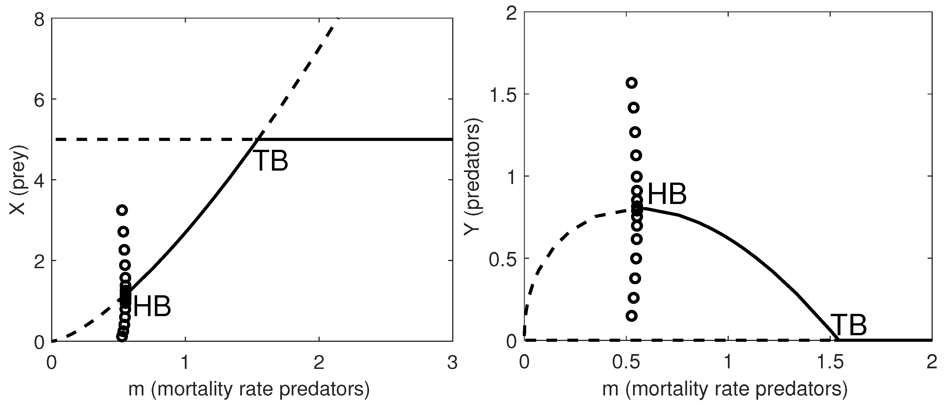
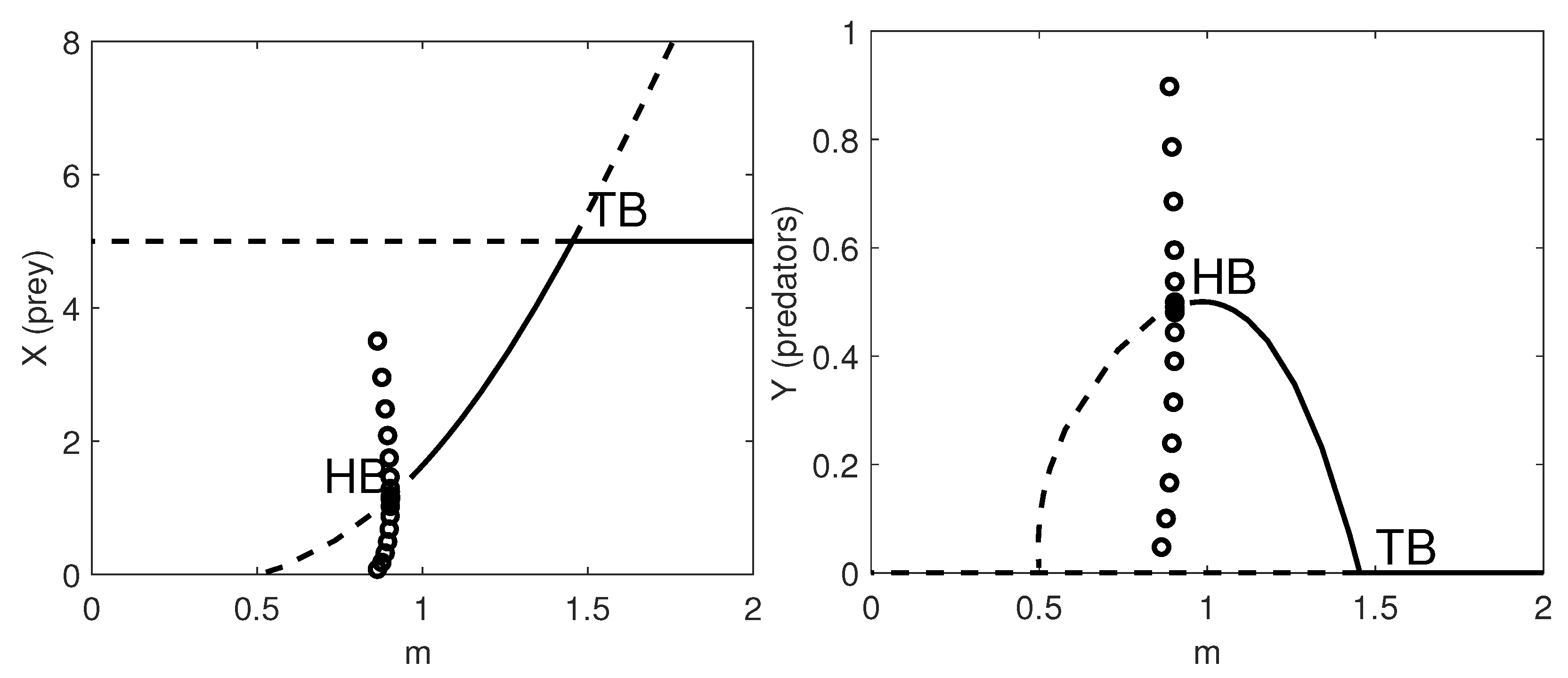
In Figure 1 we give the one-parameter bifurcation diagrams with respect to the natural mortality rate of the predators, m. Note that when m = 0.5526 , the system undergoes a supercritical Hopf bifurcation (HB) and a stable limit cycle appears. At m = 1.543 , a transcritical bifurcation occurs, where the coexistence equilibrium loses its stability and the predator-free equilibrium becomes stable.
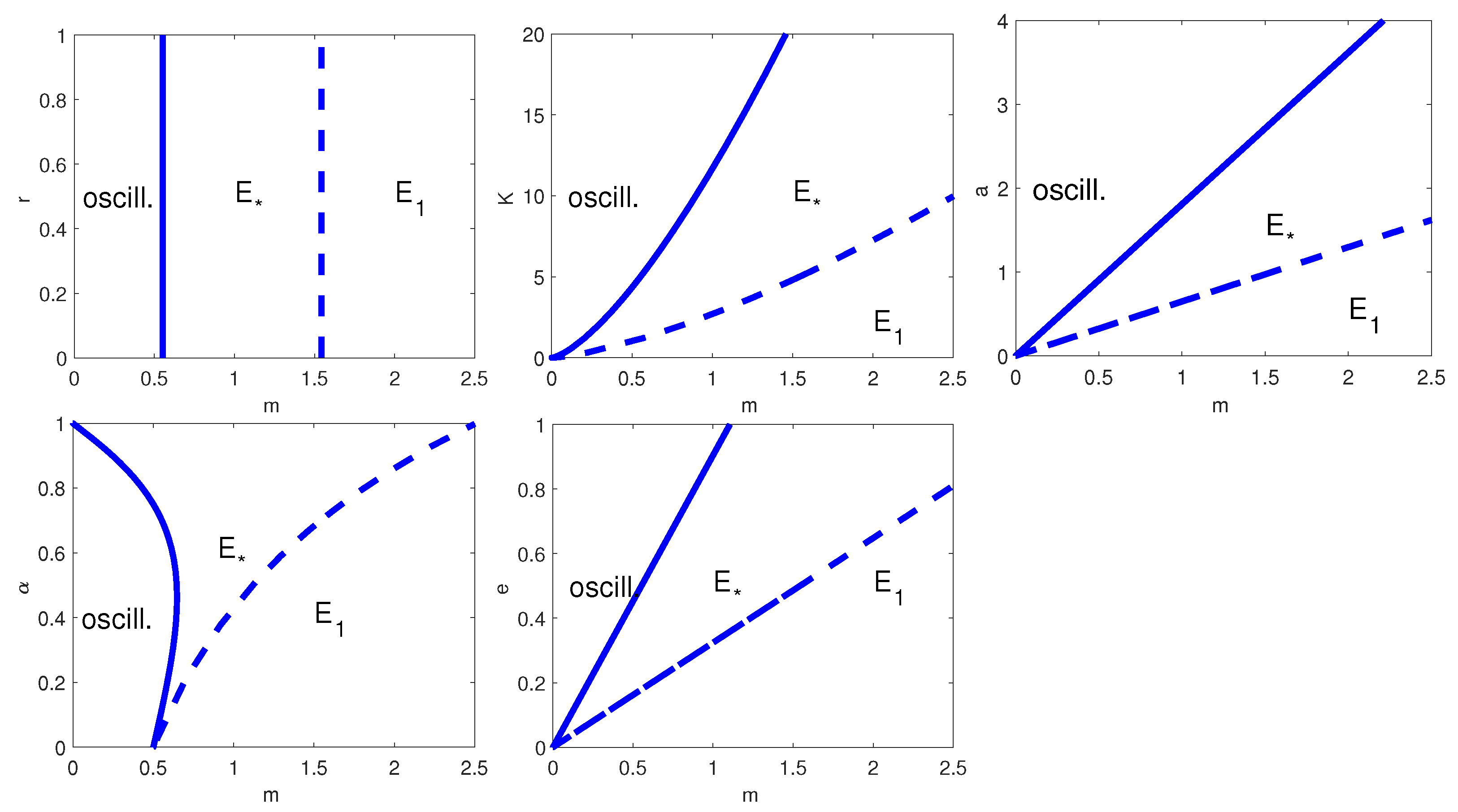
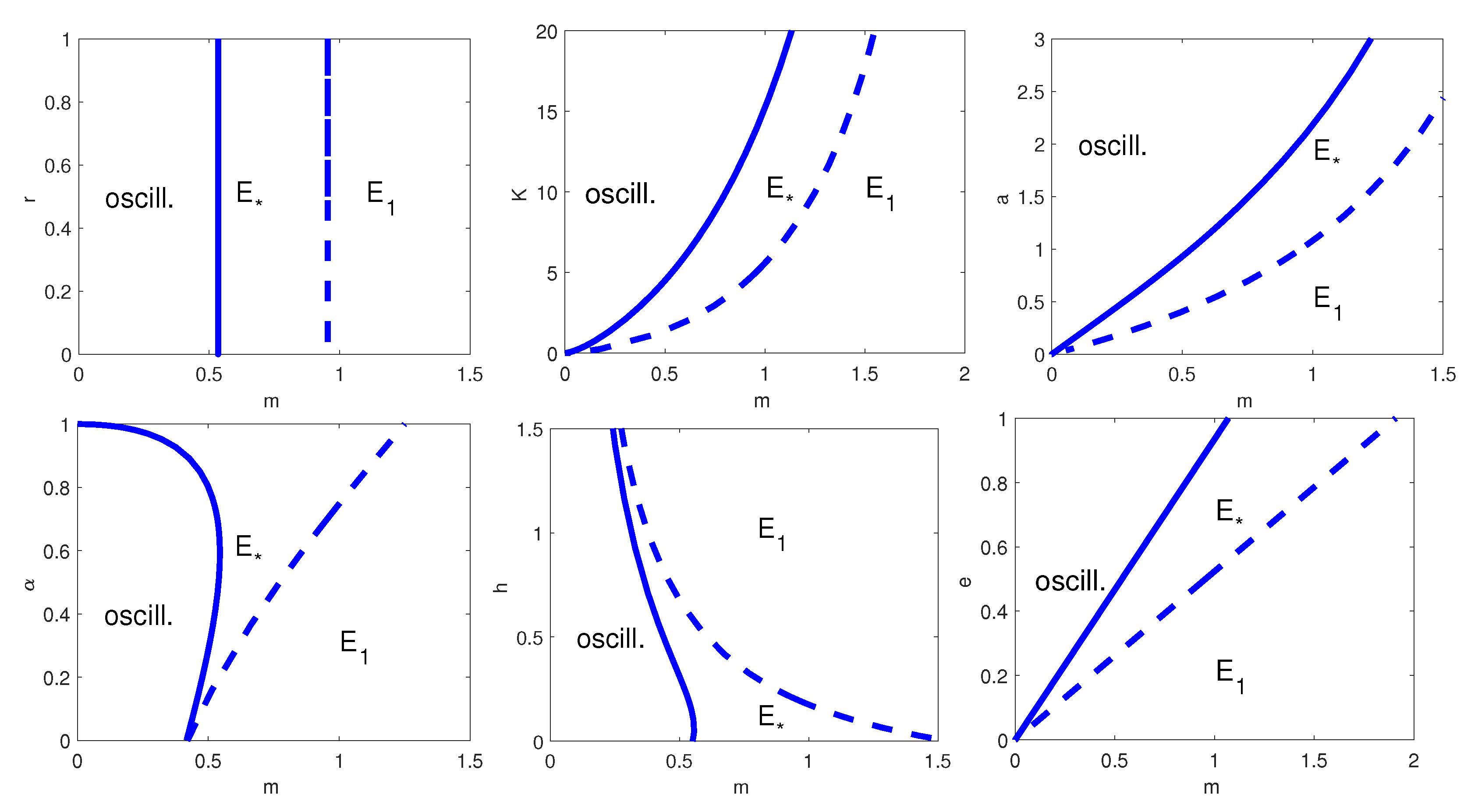
To complete the analysis, in Figure 2 we have plotted all the possible two-parameter bifurcation diagrams for ( m , 🟉 ) , with 🟉 = a , K, a, α or e. Note that the HB curve appears in all two-parameter bifurcation diagrams, but only in the plots where we vary ( m , K ) , ( m , a ) and ( m , e ) it occurs for every value of m. When we let r vary, the HB curve is present only at m = 0.5526 (Figure 2, top left); similarly, when we allow α to change, the HB occurs only for m 0.5 (Figure 2, bottom left).
As a second example, we analyse the predator–prey dynamics with generalist predator and herd-linear functional response. In Table 7 we give the nominal set of parameter values for the model in (18) and (19).
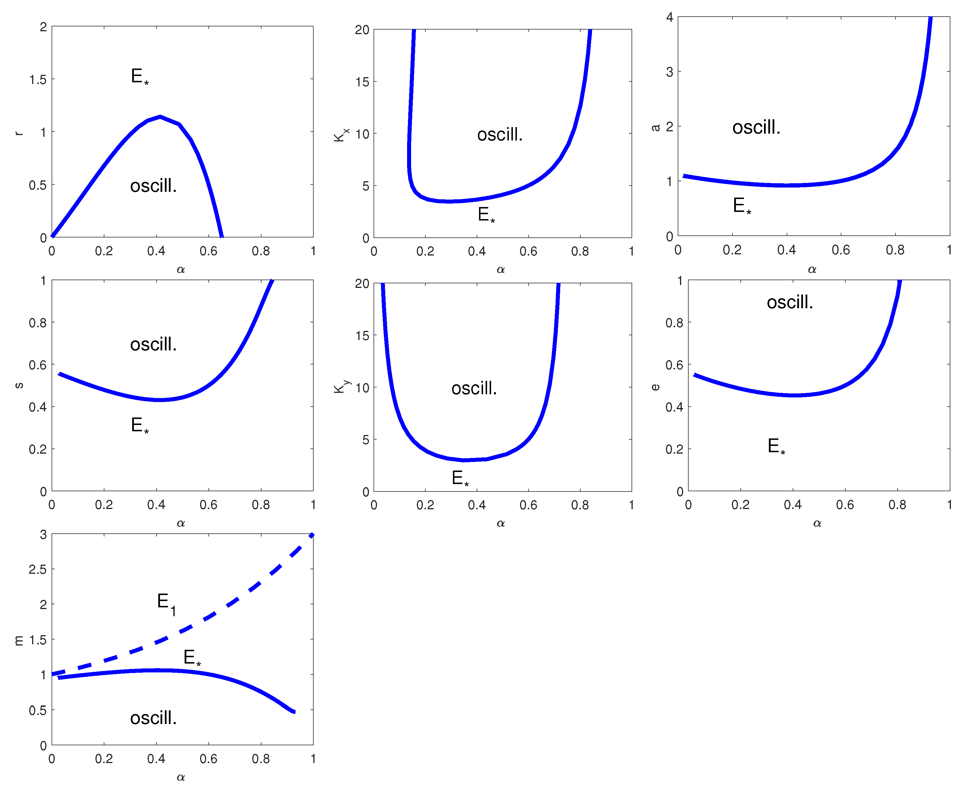
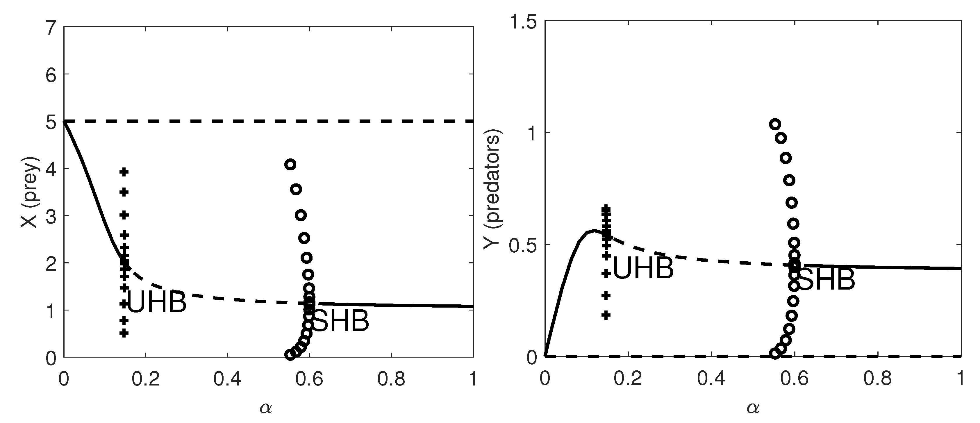
In Figure 3 we give the one-parameter bifurcation diagram with respect to the herd exponent, α . Here a supercritical HB occurs at α = 0.5995 and a subcritical HB appears at α = 0.1476 .
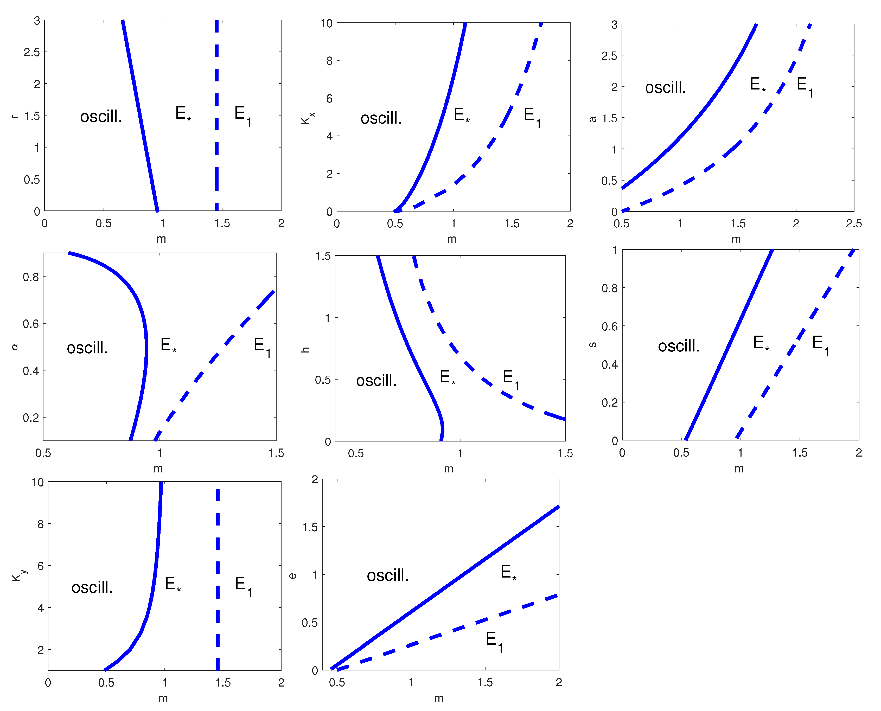
The two-parameters bifurcation diagrams with respect to ( α , 🟉 ) , with 🟉 = r , K x , a, s, K y , e, and m for the model with Equations (18) and (19) are given in Figure 4. When we vary the parameter pair ( α , a ) , a HB appears for all values of α independently of the value of a, while for the remaining cases the HB is present only for some parameter values. Moreover, we observe that only when we vary the parameter pair ( α , m ) , the transcritical bifurcation curve is present. Finally, if one of the parameters 🟉 = K x , a, s, K y , and e are below certain threshold values, with the other parameter values fixed as in Figure 4, the coexistence equilibrium is asymptotically stable; analogously, when r is above a certain threshold value the system converges to the interior equilibrium.
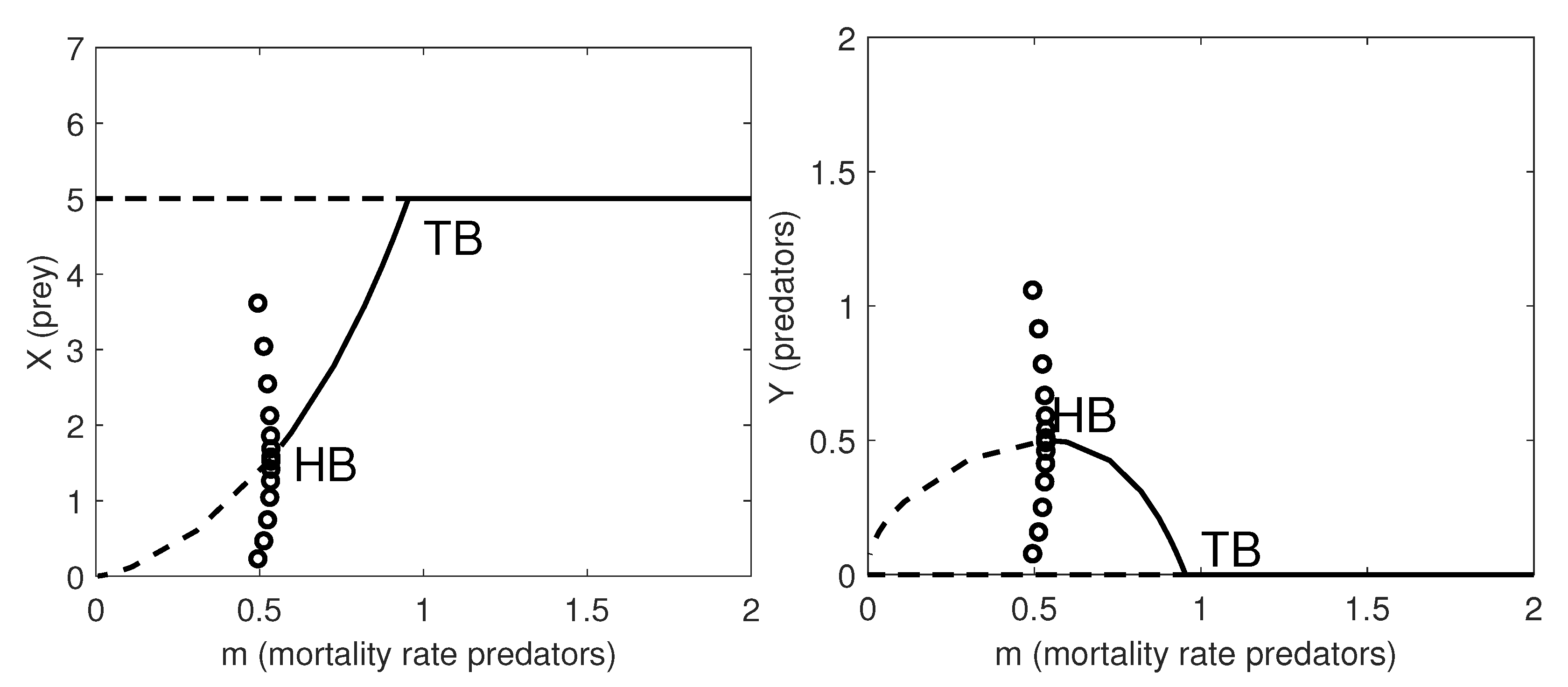
In this paragraph, we focus on the predator–prey dynamics with specialist predator and herd-Holling type II functional response. In Table 8 we list the parameter values for the model in (34) and (35).
In Figure 5 we obtain qualitatively similar results as for (6) and (7) for the one-parameter bifurcation diagrams with respect to the natural mortality rate of the predators, m.
The dynamic described in Figure 6 is similar to the one in Figure 2. There are two main differences: in the two-parameter bifurcation diagrams with respect to ( m , K ) and ( m , a ) the HB curve is more concave; when we vary the parameter pair ( m , h ) (this case is not present in Figure 2), one can see that the HB occurs for all values of h and for m smaller than a threshold value.
Finally, we study the predator–prey dynamics with generalist predator and herd-Holling type II functional response. In Table 9 we list the nominal set of parameter values for model in (42) and (43). This is the most general model that we study which encompasses all the previously considered cases.
Both the one-parameter bifurcation diagram with respect to m, and two-parameter bifurcation diagrams with respect to ( m , 🟉 ) , with 🟉 = r , K x , a, α , h, s, K y and e show behaviours similar to the previous models, see Figure 7 and Figure 8, respectively. It is worth noting that the results for models (34) and (35) are different as we give the two-parameter bifurcation diagrams with respect to the herd exponent as first parameter, while we refer to the predator natural mortality rate in the other two-parameter bifurcation plots.

4. Conclusions

The aim of this paper is to formalise, by means of illustrative examples, how prey herd behaviour can be modelled with ordinary differential equations from first principles. We propose four different Rosenzweig–MacArthur predator–prey models where the prey gather in herds and only the individuals on the edge are subjected to the predators’ attacks.
We use the mechanistic approach and time-scale separation method to derive from the individual mechanisms a Holling type II–like functional response for the predators, the herd-Holling type II functional response, which takes into account the prey herd shape. As strongly emphasised in [11,12,13,14,15], the strength of the mechanistic approach lies in the possibility of interpreting the population equations in terms of individual state transition parameter rates.
Moreover, by introducing the so-called herding index  α (see [5,6,7,8,9,10]), we model the density of the prey x on the edge of the herd as x α and we are able to track information on the herd shape in a simple system of ordinary differential equations for the population dynamics.
We focus our attention on the ecological dynamics with one prey and one predator species, including specialist versus generalist predators, i.e., no predators’ intraspecific competition versus predators’ intraspecific competition. Such antagonistic behaviour has been widely observed in population ecology, especially in aquatic species and insects, and has been proven to deeply affect niche expansion and speciation (see, for example, [19,20,21,22,23]). We further assume either herd-linear or herd-Holling type II functional responses for the predators.
Unlike the two simple cases with specialist predator where both the analytical and numerical results on the attractors and bifurcations for the population dynamics given in this paper are exhaustive, for the two models assuming intraspecific competition there is room for a more detailed study. Indeed, we have found that such ecological dynamics can give rise to multiple stable attractors (cycles and steady states), while our current analysis comprises only the cases with one interior equilibrium.
Moreover, given the evidence of possible chaotic behaviour in models with prey herd behaviour, as found for instance in the recent paper [24], the analysis can be widened in both analytical and numerical directions, by introducing an adequate change of variable. This has the advantage of simplifying the exponential term in the population equations as in [7] and analysing two-bifurcation diagrams in the same way as performed in [25].
Further extensions of our models may include more complex types of predators and prey-predator dynamics, e.g., generalist predators with respect to prey switching and prey–predator–superpredator models, where the superpredator species feeds on the prey and alternative food sources, such as cannibalising the weaker and younger predator individuals (see, for example, the state transitions and time-scale separation in [26,27] for a system with one predator species with cannibalistic tendencies). However, the greater the number of states and state transitions, the more complicated the population dynamics. Extending the mechanistic derivation of the population equations from individual-level interactions to ecosystems with multiple prey and predator species can further increase the complexity of the model, which may become parameter-heavy and will require advanced numerical methods.

Author Contributions

Formal analysis, C.B.; investigation, C.B. and I.M.B.; methodology, C.B., I.M.B. and E.V.; software, I.M.B.; writing—review and editing, C.B., I.M.B. and E.V. All authors have read and agreed to the published version of the manuscript.

Funding

C. Berardo was supported by the Academy of Finland, Centre of Excellence in Analysis and Dynamics Research. I. M. Bulai was supported by MIUR through PON-AIM Linea 1 (AIM1852570-1).

Institutional Review Board Statement

Not applicable.

Informed Consent Statement

Not applicable.

Data Availability Statement

Not applicable.

Acknowledgments

This research has been accomplished within the UMI Group TAA ”Approximation Theory and Application”.

Conflicts of Interest

The authors declare no conflict of interest.

References

  1. Laurie, H.; Venturino, E.; Bulai, I.M. Herding Induced by Encounter Rate, with Predator Pressure Influencing Prey Response. Curr. Trends Dyn. Syst. Biol. Nat. Sci. 2020, 21, 63. [Google Scholar]
  2. Liu, W.M.; Hethcote, H.W.; Levin, S.A. Dynamical behavior of epidemiological models with nonlinear incidence rates. J. Math. Biol. 1987, 25, 359–380. [Google Scholar] [CrossRef]
  3. Bhattacharyya, R.; Mukhopadhyay, B. On an epidemiological model with nonlinear infection incidence: Local and global perspective. Appl. Math. Model. 2011, 35, 3166–3174. [Google Scholar] [CrossRef]
  4. Materassi, M. Some fractal thoughts about the COVID-19 infection outbreak. Chaos Solitons Fract. X 2019, 4, 100032. [Google Scholar] [CrossRef]
  5. Ajraldi, V.; Pittavino, M.; Venturino, E. Modelling herd behavior in population systems. Nonlinear Anal. Real World Appl. 2011, 12, 2319–2338. [Google Scholar] [CrossRef]
  6. Gimmelli, G.; Kooi, B.W.; Venturino, E. Ecoepidemic models with prey group defense and feeding saturation. Ecol. Complex. 2015, 22, 50–58. [Google Scholar] [CrossRef] [Green Version]
  7. Bulai, I.M.; Venturino, E. Shape effects on herd behavior in ecological interacting population models. Math. Comput. Simul. 2017, 141, 40–55. [Google Scholar] [CrossRef]
  8. Djilali, S. Impact of prey herd shape on the predator-prey interaction. Chaos Solitons Fract. 2019, 120, 139–148. [Google Scholar] [CrossRef]
  9. Bentout, S.; Djilali, S.; Kumar, S. Mathematical analysis of the influence of prey escaping from prey herd on three species fractional predator-prey interaction model. Phys. A Stat. Mech. Its Appl. 2021, 572, 125840. [Google Scholar] [CrossRef]
  10. Djilali, S.; Ghanbari, B. Dynamical behavior of two predators–one prey model with generalized functional response and time-fractional derivative. Adv. Differ. Equ. 2021, 2021, 235. [Google Scholar] [CrossRef]
  11. Berardo, C.; Geritz, S.; Gyllenberg, M.; Raoul, G. Interactions between different predator–prey states: A method for the derivation of the functional and numerical response. J. Math. Biol. 2020, 80, 2431–2468. [Google Scholar] [CrossRef]
  12. Geritz, S.; Gyllenberg, M. A mechanistic derivation of the De Angelis-Beddington functional response. J. Theor. Biol. 2012, 314, 106–108. [Google Scholar] [CrossRef] [PubMed]
  13. Geritz, S.A.H.; Gyllenberg, M. Group defence and the predator’s functional response. J. Math. Biol. 2013, 66, 705–717. [Google Scholar] [CrossRef] [PubMed]
  14. Geritz, S.A.H.; Gyllenberg, M. The De Angelis-Beddington functional response and the evolution of timidity of the prey. J. Theor. Biol. 2014, 359, 37–44. [Google Scholar] [CrossRef] [PubMed]
  15. Metz, J.A.; Diekmann, O. The Dynamics of Physiologically Structured Populations; Springer: Berlin, Germany, 1986; Volume 68. [Google Scholar]
  16. Rosenzweig, M.L.; MacArthur, R.H. Graphical representation and stability conditions of predator-prey interactions. Am. Nat. 1963, 97, 209–223. [Google Scholar] [CrossRef]
  17. Gause, G.F. The Struggle for Existence; Williams and Wilkins: Baltimore, MD, USA, 1934. [Google Scholar]
  18. Gause, G.F.; Smaragdova, N.P.; Witt, A.A. Further studies of interaction between predators and prey. J. Anim. Ecol. 1936, 5, 1–18. [Google Scholar] [CrossRef] [Green Version]
  19. Dieckmann, U.; Doebeli, M. On the origin of species by sympatric speciation. Nature 1999, 400, 354–357. [Google Scholar] [CrossRef] [PubMed] [Green Version]
  20. Bolnick, D.I. Intraspecific competition favours niche width expansion in Drosophila melanogaster. Nature 2001, 410, 463–466. [Google Scholar] [CrossRef] [PubMed]
  21. Svanbäck, R.; Bolnick, D.I. Intraspecific competition drives increased resource use diversity within a natural population. Proc. R. Soc. B Biol. Sci. 2007, 274, 839–844. [Google Scholar] [CrossRef]
  22. Araújo, M.S.; Guimaraes, P.R., Jr.; Svanbäck, R.; Pinheiro, A.; Guimarães, P.; Reis, S.F.D.; Bolnick, D.I. Network analysis reveals contrasting effects of intraspecific competition on individual vs. population diets. Ecology 2008, 89, 1981–1993. [Google Scholar] [CrossRef] [Green Version]
  23. Bolnick, D.I. Can intraspecific competition drive disruptive selection? An experimental test in natural populations of sticklebacks. Evolution 2004, 58, 608–618. [Google Scholar] [CrossRef] [PubMed]
  24. Kumar, S.; Kumar, R.; Cattani, C.; Samet, B. Chaotic behaviour of fractional predator-prey dynamical system. Chaos Solitons Fract. 2020, 135, 109811. [Google Scholar] [CrossRef]
  25. Butusov, D.; Ostrovskii, V.; Tutueva, A.; Savelev, A. Comparing the algorithms of multiparametric bifurcation analysis. In Proceedings of the 2017 XX IEEE International Conference on Soft Computing and Measurements (SCM), St. Petersburg, Russia, 24–26 May 2017; pp. 194–198. [Google Scholar] [CrossRef]
  26. Lehtinen, S.O.; Geritz, S.A. Cyclic prey evolution with cannibalistic predators. J. Theor. Biol. 2019, 479, 1–13. [Google Scholar] [CrossRef] [PubMed]
  27. Lehtinen, S.O.; Geritz, S.A. Coevolution of cannibalistic predators and timid prey: Evolutionary cycling and branching. J. Theor. Biol. 2019, 483, 110001. [Google Scholar] [CrossRef] [PubMed]
Figure 1. One-parameter bifurcation diagram with respect to m. Left panel: the prey population dynamics. Right panel: the predator population dynamics. Thick lines: stable equilibria; dashed lines: unstable equilibria; HB: supercritical Hopf bifurcation point where a stable limit cycle arises with maximum amplitude given by the amplitude of the HB (circles); TB: transcritical bifurcation point where the coexistence equilibrium exchanges its stability with the prey-only equilibrium. The remaining parameter values are as in Table 6.
Mathematics 09 02555 g001
Figure 2. Two-parameter bifurcation diagrams with respect to m and, from top-left to bottom-right, r, K, a, α and e. Thick line: HB curve; dashed line: transcritical bifurcation curve. E is the coexistence equilibrium and E 1 the prey-only equilibrium. The remaining parameter values are as in Table 6.
Mathematics 09 02555 g002
Figure 3. One-parameter bifurcation diagram with respect to α . Left panel: the prey population dynamics. Right panel: the predator population dynamics. Thick lines: stable equilibria; dashed lines: unstable equilibria; SHB: supercritical Hopf bifurcation point where a stable limit cycle arises with maximum amplitude given by the amplitude of the SHB (circles); UHB: subcritical Hopf bifurcation point, where an unstable limit cycle arises with maximum amplitude given by the amplitude of the UHB (pluses); TB: transcritical bifurcation point where the coexistence equilibrium exchanges its stability with the prey-only equilibrium. The remaining parameter values are as in Table 7.
Mathematics 09 02555 g003
Figure 4. Two-parameter bifurcation diagram with respect to α , and, from top left to bottom right, r, K x , a, s, K y , e and m. Thick line: HB curve; dashed line: transcritical bifurcation curve. E is the coexistence equilibrium and E 1 the prey-only equilibrium. The remaining parameter values are as in Table 7.
Mathematics 09 02555 g004
Figure 5. One-parameter bifurcation diagram with respect to the natural mortality rate of the predators, m. Left panel: the prey population dynamics; Right panel: the predator population dynamics. Thick lines: stable equilibria; dashed lines: unstable equilibria. HB: supercritical Hopf bifurcation point where a stable limit cycle arises with maximum amplitude given by the amplitude of the HB (circles); TB: transcritical bifurcation point where the coexistence equilibrium exchanges its stability with the prey-only equilibrium. The remaining parameter values are as in Table 8.
Mathematics 09 02555 g005
Figure 6. Two-parameter bifurcation diagram with respect to m and, from top left to bottom right, r, K, a, α , h and e. Thick line: HB curve; dashed line: transcritical bifurcation curve. E is the coexistence equilibrium and E 1 the prey-only equilibrium. The remaining parameter values are as in Table 8.
Mathematics 09 02555 g006
Figure 7. One-parameter bifurcation diagram with respect to m. Left panel: the prey population dynamics. Right panel: the predator population dynamics. Thick lines: stable equilibria; dashed lines: unstable equilibria; HB: supercritical Hopf bifurcation point where a stable limit cycle arises with maximum amplitude given by the amplitude of the HB (circles); TB: transcritical bifurcation point where the coexistence equilibrium exchanges its stability with the prey-only equilibrium. The remaining parameter values are as in Table 9.
Mathematics 09 02555 g007
Figure 8. Two-parameters bifurcation diagram with respect to m and, from top left to bottom right, r, K x , a, α , h, s, K y , and e. Thick line: HB curve; dashed line: transcritical bifurcation curve. E is the coexistence equilibrium and E 1 the prey-only equilibrium. The remaining parameter values are as in Table 9.
Mathematics 09 02555 g008
Table 1. Conditions for feasibility and stability of the equilibria of the system in (12) and (13). The trivial equilibrium E 0 is always unstable. TB: transcritical bifurcation. HB: Hopf bifurcation.
Condition E 1 E Bifurcation
m a e > 1 asympt. stablenot feasible
m a e = 1 TB
α 1 α 2 α < m a e < 1 unstableasympt. stable
m a e = α 1 α 2 α HB
0 < m a e < α 1 α 2 α unstableunstable
Table 2. Conditions for the feasibility and stability of the equilibria of the system in (23) and (24).
Condition E 0 E 1 E 2 E 1 E 2
m < s unstableunstableunstableSee Table 3See Table 3
s < m < s + a e unstableunstablenot feas.stablenot feasible
m > s + a e unstableasympt. stablenot feasiblenot feasiblenot feasible
Table 3. Conditions for feasibility of the interior equilibria of the system in (23) and (24) when m < s .
Condition E 1 E 2
1 m s < 1 a ( 2 α ) 1 α 2 α 1 α e a s 1 α 2 α α feasiblefeasible
1 m s = 1 a ( 2 α ) 1 α 2 α 1 α e a s 1 α 2 α α feasiblenot feasible
1 m s > 1 a ( 2 α ) 1 α 2 α 1 α e a s 1 α 2 α α not feasiblenot feasible
Table 4. Conditions for feasibility and stability of the equilibria of the system in (37) and (38). TB: transcritical bifurcation. HB: Hopf bifurcation.
Condition E 0 E 1 E Bifurcation
e a < m a h + m unstableasympt. stablenot feasible
e a = m a h + m TB
e a > m a h + m , g ( x ) f ( x ) < 0 unstableunstableasympt. stable
e a > m a h + m , g ( x ) f ( x ) = 0 HB
e a > m a h + m , g ( x ) f ( x ) > 0 unstableunstableunstable
Table 5. Conditions for feasibility and stability of the trivial equilibria of the system in (45) and (46).
Condition E 0 E 1 E 2
m < s + e a 1 + a h unstableunstableunstable
m > s + e a 1 + a h , g ( x ) f ( x ) < 0 unstableasympt. stableunstable
Table 6. Nominal set of parameter values for the model in (6) and (7).
ParameterDescriptionValue
rprey net reproduction rate1
Kprey carrying capacity5
apredation rate1
α herd exponent 0.7
econversion factor 0.5
mnatural mortality rate (predators)1
Table 7. Nominal set of parameter values for the model in (18) and (19).
ParameterDescriptionValue
rprey net reproduction rate 0.5
K x prey carrying capacity5
apredation rate1
α herd exponent 0.7
spredator reproduction rate 0.5
K y predator carrying capacity5
econversion factor 0.5
mnatural mortality rate (predators)1
Table 8. Nominal set of parameter values for the model in (34) and (35).
ParameterDescriptionValue
rprey net reproduction rate 0.5
Kprey carrying capacity5
apredation rate1
α herd exponent 0.7
hhandling time 0.2
econversion factor 0.5
mnatural mortality rate (predators)1
Table 9. Nominal set of parameter values for the third model (42) and (43).
ParameterDescriptionValue
rprey net reproduction rate 0.5
K x prey carrying capacity5
apredation rate1
α herd exponent 0.7
hhandling time 0.2
spredator reproduction rate 0.5
K y predator carrying capacity5
econversion factor 0.5
mnatural mortality rate (predators)1
Publisher’s Note: MDPI stays neutral with regard to jurisdictional claims in published maps and institutional affiliations.

