Modeling and Analysis of Cardiac Hybrid Cellular Automata via GPU-Accelerated Monte Carlo Simulation

Abstract

The heart consists of a complex network of billions of cells. Under physiological conditions, cardiac cells propagate electrical signals in space, generating the heartbeat in a synchronous and coordinated manner. When such a synchronization fails, life-threatening events can arise. The inherent complexity of the underlying nonlinear dynamics and the large number of biological components involved make the modeling and the analysis of electrophysiological properties in cardiac tissue still an open challenge. We consider here a Hybrid Cellular Automata (HCA) approach modeling the cardiac cell-cell membrane resistance with a free variable. We show that the modeling approach can reproduce important and complex spatiotemporal properties paving the ground for promising future applications. We show how GPU-based technology can considerably accelerate the simulation and the analysis. Furthermore, we study the cardiac behavior within a unidimensional domain considering inhomogeneous resistance and we perform a Monte Carlo analysis to evaluate our approach.

1. Introduction

Computational cardiology provides a safe, non-invasive, and ethical method to investigate the heart and its dysfunctionalities. Early mathematical models [1,2,3,4] extend the pioneering work of Hodgkin-Huxley [5] to describe and explain, with a set of ordinary differential equations (ODEs), the ionic mechanisms responsible for the initiation and the electrical propagation of action potentials traversing excitable cells such as cardiac myocytes and neurons [6,7]. These early studies enabled innovative in-silico research and clinically oriented applications [8]. For example, they allow us to understand a variety of nonlinear phenomena affecting cardiac dynamics [9,10,11,12,13] and unexpected, chaotic properties of the heart [14,15]. The mathematical complexity of such models has stimulated several works [16,17,18] trying to improve the analysis by simplifying the model representation.

Cellular Automata (CA) are a well-known class of discrete simplified dynamical systems widely used to reproduce pattern formation and growth [19,20]. One of the first approaches using CA and its theory was proposed by von Neumann et al. [21]. A cellular automaton consists of a regular grid of cells where a discrete state is associated to each cell. The state of each cell can evolve in time according to a set of rules operating over the states of the neighboring cells. This class of models provides a simple mathematical framework to reproduce several emergent behaviors that can be observed in excitable media such as the cardiac tissue [22] and the nervous system [23]. Other extensions of CA allow one to customize the model describing how each cell reacts to the external stimuli from the neighboring cells. For example, the electrophysiological process in a myocyte is driven by a set of voltage-dependent thresholds that control the opening/closing of ionic channels regulating the flux of ions across the cellular membrane. These thresholds generally identify specific phases of the myocyte’s behavior, such as the rapid depolarization, the initial repolarization, the plateau, and the late repolarization/resting phase, characterized by different dynamics.

A well-established approach to describe such processes is via Hybrid Automata [24,25,26], a modeling formalism that extends finite automata with a set of ODEs describing the continuous behavior of the action potential at each phase (a phase corresponds to a discrete state in the finite automata). A set of guard conditions over voltage-dependent thresholds determine how each cell switches the continuous dynamics that modeling the inward/outward flux of ionic currents at each phase. Previous works [24,25,27] have shown that HA can accurately reproduce the action potential occurring in myocytes. HA can be simulated using numerical integration, but they are also amenable to formal analysis techniques such as model checking [18,28]. HA and CA can be then combined in a Hybrid Cellular Automata (HCA) that can model both the reaction of each cell to external stimuli and the diffusion of the ionic currents among neighboring cells.

In this work, we consider an HCA model where the single cell behavior is described by a simplified but very accurate four-variables hybrid model proposed in [16] and the cells are coupled with a simple link (resistance) to propagate signals as a unidirectional cable or as a ring of cardiac cells. The considered phenomenological modeling approach stems from experimental works on one-dimensional rings of cardiac cells and whole heart models studying the onset of alternans and irregular rhythms [29,30,31].

In addition to modeling, one can reduce simulation time and associated computational costs using special hardware accelerators such as Graphical Processing Units (GPU) [32,33,34] and Field Programmable Gate Arrays (FPGA) [35,36]. To optimally simulate our cardiac cell model, we compare common numerical methods in combination with different coding approaches: Matlab^®Simulink, a sequential C implementation running on a CPU and an NVIDIA^®CUDA-based implementation running on a modern GPU. Such a comparison is a required step to evaluate the limitations and trade-offs of the different technologies as well as the reliability of our modeling approach.

The literature is populated by a multitude of physiological and phenomenological mathematical models of cardiac cell electrophysiology [37]. These dynamical systems are usually analyzed in terms of local restitution features (e.g., changes of the action potential duration versus decreasing stimulation pacing periods) as well as bifurcation diagrams (when period-doubling occurs) and space-time visualization [38,39,40,41,42]. Like the biological original, models depend on a variety of additional parameters, i.e., including temperature, membrane resistance, and nonlinearities within the tissue [11,43,44,45].

One-dimensional cables and rings of cardiac cells fulfill standard physiology studies on reentry circuits in cardiology [46,47]. Monolayers of cardiomyocytes [29], as well as multiorgan structures [30], introduced a fine control of system’s dynamics improving our understanding of complex neurocardiac diseases. Due to certain pathological conditions, such as ischemia, current sinks might develop. This behavior can be simulated by changing the amount of heterogeneity within the tissue and the coupling between cells [48]. In this perspective, we will conduct an extended analysis investigating emergent phenomena associated with alternans and conduction blocks by using bifurcation diagrams and modeling the cell-cell coupling with a random variable. First, we investigate the propagation and benchmarks of our model, with respect to conduction velocity (CV) and action potential duration (APD). Then we analyze the resiliency of the proposed HCA by decreasing the length (cell count) within the ring structure after a freely chosen amount of time-steps. Doing so, we achieve shortening and spatiotemporal adaptation of the excitation wave, without the need of electrical pacing, also observing the onset of electrical alternans.

The final object of the paper is to assess the proposed HCA approach under different implementations. We do so by investigating the results of a Monte Carlo simulation analysis. As we are using a free resistance variable, we test the robustness of the approach using random values for this variable. We then use a numerical analysis of the bifurcation over APD in a decreasing number of cells. This study allows us to draw conclusions on usability, deficiencies, and further improvement of HCA as a cardiac modeling technique.

The paper is structured as follows: we first present the considered computational models and analysis techniques in Section 2. In Section 3, we summarize the main findings of our computational experiments, and we compare the performance of different model implementations. We discuss our results in Section 4. We conclude in Section 5 by discussing limitations and perspectives of our work.

2. Computational Models and Methods

In this section, we present the computational models that we have considered in our analysis and different computational approaches to simulate them.

2.1. Unidirectional Hybrid Cellular Automata Model

The presented HCA model satisfies the properties of a Cellular Automata by following simple principles: each node represents a cell and the smallest entity of an HCA, which can have different states. The state of a cell depends on the states of its neighbors in the previous step, leading to a unidirectional coupling between cardiac cells.

For the determination of the cell state, we are using the four-variable phenomenological Minimal Model [16], recapitulated in Equations (1) and (2), adopting the minimum set of ODEs to recover specific cardiac behaviors, e.g., action potential shape and duration, restitution properties, conduction velocity, and alternans dynamics [49,50]:

$$\begin{array}{cc}\hfill {\partial }_{t}u& =\nabla ·(\tilde{D}\nabla u)-(j_{fi}+j_{so}+j_{si})+j_{ext}\hfill \\ \hfill {\partial }_{t}v& =(1-H(u-{\theta }_v))(v_{\infty }-v)/{\tau }_v^{-}-H(u-{\theta }_v)v/{\tau }_v^{+}\hfill \\ \hfill {\partial }_{t}w& =(1-H(u-{\theta }_w))(w_{\infty }-w)/{\tau }_w^{-}-H(u-{\theta }_w)w/{\tau }_w^{+}\hfill \\ \hfill {\partial }_{t}s& =(1-tanh\left(k_s(u-u_s)\right))/2-s)/{\tau }_s\hfill \end{array}$$

(1)

$$\begin{array}{cc}\hfill j_{fi}& =-vH(u-{\theta }_v)(u-{\theta }_v)(u_u-u)/{\tau }_{fi}\hfill \\ \hfill j_{so}& =(u-u_o)(1-H(u-{\theta }_w))/{\tau }_o+H(u-{\theta }_w)/{\tau }_{so}\hfill \\ \hfill j_{si}& =H(u-{\theta }_w)ws/{\tau }_{si}\hfill \end{array}$$

(2)

Equation (1) lists the four state-variables reaction-diffusion dynamics, where u is the normalized transmembrane voltage variable and $v,w$, and s are normalized virtual gates, namely gating variables, ranging between 1 and 0. These gating variables are a phenomenological equivalent of ion-channels kinetics within a cell and used to compute the three currents listed in Equation (2): fast inward, $j_{fi}$, slow inward, $j_{si}$ and slow outward, $j_{so}$. Such a phenomenological description has been proved to recreate the spatiotemporal action potential features of cardiac cells and tissues. In particular, the diffusion term $\nabla ·(\tilde{D}\nabla u)$ allows for cell-cell signal transmission in space, where $\tilde{D}$ represents the diffusion coefficient based on human ventricular tissue experiments. Finally, an external time-dependent stimulation current, $j_{ext}$, is added to the ionic currents to reproduce electrical pacing of the tissue and H is the standard Heaviside function.

Model parameters, defining time-constants and threshold values, refer to epicardial cells behavior (see Appendix A). More precisely, the constant values are listed in

Table A1. Model Parameters.

${\mathit{\tau }}_{\mathit{v}}^{+}$	${\mathit{\tau }}_{1\mathit{v}}^{-}$	${\mathit{\tau }}_{2\mathit{v}}^{-}$	${\mathit{\tau }}_{\mathit{w}}^{+}$	${\mathit{\tau }}_{1\mathit{w}}^{-}$	${\mathit{\tau }}_{2\mathit{w}}^{-}$	${\mathit{\tau }}_{\mathit{s}1}$	${\mathit{\tau }}_{\mathit{s}2}$	${\mathit{\tau }}_{\mathit{f}\mathit{i}}$	${\mathit{\tau }}_{\mathit{o}1}$	${\mathit{\tau }}_{\mathit{o}2}$
1.4506	60	1150	200	60	15	2.7342	16	0.11	400	6
${\theta }_{v_{\infty }}$	${\theta }_w$	${\theta }_{w_{\infty }}$	${\theta }_{so}$	${\theta }_{si}$	${\theta }_o$	${\tau }_{so1}$	${\tau }_{so2}$	${\tau }_{si}$	${\tau }_{w_{\infty }}$	${\theta }_v$	${\theta }_v^{-}$
0.006	0.13	0.006	0.13	0.13	0.006	30.0181	0.9957	1.8875	0.07	0.3	0.006
$k_w^{+}$	$k_w^{-}$	$k_s$	$k_{so}$	$k_{si}$	$u_w^{-}$	$u_s$	$u_o$	$u_u$	$u_{so}$	$w_{\infty }^{\ast }$
5.7	65	2.0994	2.0458	97.8	0.03	0.9087	0	1.55	0.65	0.94

, the determination for the varying definitions are shown in Equation (A1) and the infinity values in Equation (A2). According to [16,51] the critical parameters ruling system’s features include, amongst others, the maximum AP upstroke velocity (via ${\tau }_{fi},{\tau }_v^{+},{\theta }_v$ ), AP amplitude (via $u_u,u_o$), maximum and minimum APD (via ${\tau }_w^{+},{\tau }_{si},{\tau }_{so}$).

The local state of a cell is determined by the difference between its two neighboring cells. To control the CV and other expected physical properties of the HCA, we introduced a free variable for the cell membrane resistance. Accordingly, the computation for propagation reads:

$$\begin{array}{c}\hfill (u_{i-1}-u_i)\ast R_V\end{array}$$

(3)

where $u_i$, represents the voltage of the current cell, i, and $R_V$ the free resistance variable among cell i and cell $i-1$. Therefore, the resulting discretized reaction-diffusion equation (cable equation) for the voltage variable u becomes:

$$\begin{array}{cc}\hfill {\partial }_{t}u& =u-((u_{i-1}-u_i)\ast R_V+j_{fi}+j_{so}+j_{si})\hfill \end{array}$$

(4)

Equation (4) together with the local kinetics (1) are the mathematical foundation of the present approach, as the state of the HCA cells is represented by the four state-variables of the Minimal Model. For state-change propagation within the HCA, i.e., the update function, we use Equation (3) using the voltage-state of the predecessor in the previous time step. The activation wave in the HCA is created by setting an excited initial condition for the cell at index 0 with values $u=1,v=1,w=1$ and $s=0$. For all other cells we set instead as initial condition the values $u=0,v=1,w=1$ and $s=0$ corresponding to resting state. The state values for computation are dimensionless to recreate phenomena and not scaled to any biophysical properties or ion concentrations. According to [16], u can be scaled to mV using the equation $V_{mV}=85.7u-84$.

A highly simplified illustration of the propagation flow within the proposed HCA is shown in Figure 1. Each node represents a cell $C_x$ at position x. In particular, the first cell is activated at time step 0 (T0), the cell in the second position updates only in the next step (T1). This pattern is valid for all the cells. Due to the difference of potential between neighboring cells, the action potential u will propagate in time across all the cells. Restoration of resting (quiescent) conditions follows the cardiac action potential time constant with vanishing activation wave propagation. Figure 1 shows different shades of gray that corresponds, and we assume that at time step 2 (T2), the impulse created at $C_2$ is too weak to activate the last cell; therefore, it does not change color in Figure 1e.

2.2. Model Behavior Evaluation

The original Minimal Model by Bueno-Orovio et al. can simulate a wide range of cardiac behavioral patterns. Therefore, to evaluate our HCA model, we assess which patterns and characteristics we can recover. One of the most important benchmarks to evaluate the model, is the CV which is approximately $0.5$ $\mathrm{m}$/$\mathrm{s}$ [52]. This benchmark asserts the usability of a free resistance variable in the model, which we use to control CV. Further, we evaluate the AP propagation and its duration within the model to ensure correct physiological behavior. These benchmarks are also used to determine the optimal value for the resistance variable.

Additionally, we use highly simplified structures to evaluate the functionality and behavior of our HCA. We are using a unidirectional propagation in 1D cell structures, shown in Figure 2. The cells are a voltage source, propagating from previous to next (left to right). Between each cell is a resistor, resembling the computation of Equation (3). In Figure 2b the last cell propagates to the first cell, creating a closed ring. If a circular cell construct is stimulated at a single point, it propagates bidirectionally. Propagation waves, then, meet in the middle and extinguish each other (annihilate) [53]. If the stimulus is delivered with hyperpolarization on one site (i.e., one of the two concurring cells cannot be activated), the wave starts to propagate only in one direction, as the different state of the cells does not allow stimulation in the other. Due to connections between first and last cell (i.e., periodic boundary conditions), propagation of state-change runs in a circle. The wave is, therefore, "trapped" in our ring, showing self-sustained propagation, a prototype of cardiac reentry and arrhythmias. To simulate this one-directional wave, we designed the previously described 1D ring of cells in Figure 2b. With this unidirectional flow of waves, we are able to simulate a trapped circuit wave [54] and omit the necessity to establish a one-sided block in the opposite direction.

Figure 2a shows the cell cable, with no-flux boundary conditions, represented as a barrier at beginning and end. These two constructs will give us insights into the properties and recoverable characteristics of our model, as the ring represents the smallest closed circuit entity in cardiac arrhythmias [46]. The cable, on the other hand, gives us insight into the correct propagation properties and alternans dynamics of the presented approach.

Specifically, using 1D structures, we study CV and APD features. Further, by reducing the ring length during the simulation, we highlight the self-adapting properties of cardiac cells within a ring. To avoid unnecessary computation steps, we validate the sum of the voltage over the cable in each time step: if it falls below a value of 0.5, the simulation stops assuming that no action potential occurs. Additionally, we investigate the impact of the resistance value on our model in these scenarios. Each scenario is performed once in a homogeneous setup, with a constant resistance value for each cell. Then we introduce tissue heterogeneity using different resistance in each cell and time step. The adopted values follow the von Mises distribution, and a Monte Carlo study is performed as described below.

2.3. Computational Methods

High-performance CPUs and GPUs are the most common hardware technologies employed to simulate complex cardiac models [32]. Additionally, Matlab^®Simulink provides a suitable graphical programming framework enabling fast model prototyping and revision.

2.3.1. Matlab^®Simulink

Matlab^®Simulink is a proprietary graphical programming environment designed to model, simulate and analyze dynamical systems. It provides a graphical block diagramming language and a set of block libraries that can be easily customized by the user. Each block represents a mathematical function and the graphical environment provides the user with the possibility to build complex models by just dragging-and-dropping blocks and connecting them, without the need to have much experience in programming. Moreover, the language enables one to derive new composite blocks out of other primitive/atomic or composite blocks.

We have implemented our HCA model using this framework (see Figures in Appendix E.1). In particular, we have implemented the Minimal Model as a single Simulink block representing a cell. We then compose several cell blocks in a cable by connecting the input/output of each cell block with its neighboring cells. In Figure A1, we show the first cell of the cable, where the constant mode in this block, as well as the switch, decide if the first cell is connected to the last cell, forming a ring of cells. The computation of input connection is performed within a separate blockResistor, shown in Figure A2. The external impulse ($I_{ex}$) in both blocks represents an external stimulation (Pulse Generator block) which can be activated in the main Model block, as shown in Figure A4.

We created special block that groups a certain amount of cells block together. Using these special blocks, we were able to create and simulate structures of maximum 3000 cells. For example, in Figure A3, we show the smallest entity of five grouped cells.

2.3.2. Central Processing Unit (CPU) and Graphics Processing Unit (GPU)

Despite Matlab^®Simulink being suitable for fast model prototyping and revision, it is less efficient when it comes to handling the simulation of thousands or millions of cardiac cells. Thus, we first implemented in C-language a second version of our simulator that runs sequentially on a CPU. In this implementation, we represent the HCA model as an array of cells, avoiding the use of complex pointer-arithmetic; for example, the access to the neighboring cells and the decreasing of the cable size at runtime are performed using only integer indices instead of pointers.

We use this sequential implementation as a baseline to both check the correctness and compare the performance of a third parallel implementation that we developed to run on a GPU. GPUs are programmable chipsets with flexible throughput-oriented processing architecture and were originally designed to solve problems that require high-performance computing, such as 3D graphic renderings. Figure 3 illustrates how GPU architecture is organized around an array of streaming multiprocessors (SMs). Each SM includes several scalar processors (SPs), and each SP consists of an arithmetic logic unit that can perform a floating-point operation.

The GPU code development is generally simplified by a software layer that provides access to the instruction set and parallel computational elements of the GPU. In this work, we used the Compute Unified Device Architecture (CUDA) designed specifically for NVIDIA^®GPU cards. The CUDA parallel model enables the execution of thousands of lightweight threads organized in thread blocks. Each thread executes in parallel the code of a function called kernel while using different parameters. The threads that are within the same thread block can cooperate using different mechanisms. For example, a synchronization point in the code of the kernel makes sure that all the threads must reach that point before the execution can continue. Threads in the same block can also exchange data among each other using on-chip shared memory. Threads that are located in different blocks cannot be synchronized during the kernel execution and operate independently. The CUDA environment provides the possibility to use C/C++ languages extended with built-in primitives enabling the programmer to launch thousands of threads and to specify parameters for the threads and their blocks.

The CUDA model refers a GPU with the term device while a CPU with the term host. A device has different types of memory, and their correct use can highly impact the performance of the implementation. The global memory is a device memory that can be read/written by all the threads running on the device. The host can also access the global memory of the device using special CUDA primitives. This enables the exchange of data between the host and the device memories. The global memory is generally available in large amounts (e.g., in the order of gigabytes), but its access is also very expensive. Within the SM, there are instead two very fast (but limited in size) types of memory: the registers and the shared memory. Registers have the largest bandwidth, but very small size and can only be accessed by a single thread. They are partitioned among all the threads of a thread block running on a SM. The amount of available registers also limits the number of threads that can be executed in the same thread block. Shared memory can be accessed as fast as the registers, and it facilitates the communication among the threads in the same thread block.

In our implementation, we developed two kernels: the first calculates the diffusion of the action potential among the cells using the values of the first neighbors for each cell; the second computes the numerical integration for a time-step of the piece-wise nonlinear ordinary differential equations modeling the inward/outward current flows in each cardiac cell. The program starts with a main function running on the CPU. First, it allocates the necessary global memory space in the GPU device to store the cardiac cells, and then it initializes the simulation. This procedure is followed by a while loop terminating when the simulation is completed. At each loop iteration, the program first calls the kernel function to compute the action potential diffusion across the cells and then calls the kernel updating the values of the ionic current flows and of the action potential for each cell. When a kernel is called, its code is executed in parallel on a grid with multiple blocks of threads running on the device, one thread assigned to each cell. At the end of the execution of a kernel, the control flow returns to the CPU, and this provides an implicit point of synchronization, enabling data consistency before the launch of the threads for the next kernel. When other analysis are necessary, intermediate results can be transferred from the GPU to the CPU after multiple loop iterations. However, this operation is computationally expensive and can slow down the computation.

The work in [32] shows that the use of shared memory can increase the efficiency of the simulation when it is employed to compute the diffusion for large 2D/3D cardiac domains. However, for the simulation of a one-dimensional cable or ring of cardiac cells, we have not observed a significant increase in efficiency by using shared memory.

It is worth noting that we use a pre-generated lookup table (LUT) for the resistance variables following the von Mises distribution, as we do not have enough memory available on GPU it is only accessible on CPU. Therefore, for the GPU implementation in each step, we randomly generate an array of indices to access the LUT and read the values into another array, which is then copied onto the device, and the indices correspond to the indices of the cells. To exploit the full usage of GPU, we use cuRand, a built-in random number generation library. On the CPU, we use a similar approach to sample the resistance values, with the C-library function rand(). These functions must be initialized with a different seed to produce different sequences each time. In both versions, we use the current system time to initialize the seed. For LUT, we pre-generated several distributions with various $\kappa$ and $\mu$ for a greater sample size pool.

For reasonable results, we introduced a virtual cell size, meaning a size that one cell supposedly has in length. In all following images and representations, each cell has a length of 100 $\mathsf{\mu }$$\mathrm{m}$. The virtual cell size is mostly used to compute the CV and APD. If not said otherwise, we measure the length of the structures in the number of cells and the simulation time in time-steps per cell.

3. Results

In this section, we present the results for the different test scenarios that we have considered. All the experiments were performed on a workstation equipped with an NVIDIA^®GeForce GTX TITAN X (with 12 GB GDDR5 of memory) and an Intel^®Core^TM i7-5820K CPU (with 32 GB of RAM). We used Matlab^®version 2019b, including the full toolbox set for Simulink. The sample size is determined by the number of cells in the HCA as well as the number of performed time-steps in the simulations without decreasing size.

3.1. Accuracy of GPU

We assume the calculations in the CPU-based implementation are correct. To determine the correctness and truncation error and hence resulting loss of accuracy, we computed the mean squared error, E, comparing the voltage values obtained by simulating a cell cable with both the GPU-based ($\overline{u}$) and CPU-based ($\widehat{u}$) implementations:

$$E=\frac{1}{N\ast T}\sum _{s=0}^{N-1}\sum _{t=0}^{T-1}{({\widehat{u}}_t^s-{\overline{u}}_t^s)}^2,$$

(5)

where N refers to the number of cells and T to the simulation time in time-steps computed per cell. As Figure 4 shows, the error is negligible for a variety of resistance variables, number of cells, and simulation time (i.e.,: 20,000 steps ~1 s, as 1 step = 0.05 ms). In Figure 4a the boxplot was computed for each $R_V$ in

Table A2. MSE of u between CPU and GPU Sample size as number of cells times simulation time (in time-steps) on the Left Value of the $R_V$ on Top.

Sample Size|${\mathbf{R}}_{\mathbf{V}}$	0.5	1.7	2.0	2.2	3.0	3.5
$\mathbf{1000}\ast$20,000	3 $\times {10}^{-6}$	3 $\times {10}^{-6}$	1 $\times {10}^{-6}$	0.0	0.0	0.0
$\mathbf{1000}\ast$30,000	8 $\times {10}^{-6}$	3 $\times {10}^{-6}$	2 $\times {10}^{-6}$	0.0	0.0	0.0
$\mathbf{1000}\ast$40,000	1 $\times {10}^{-5}$	2 $\times {10}^{-6}$	5 $\times {10}^{-6}$	3 $\times {10}^{-6}$	0.0	0.0
$\mathbf{2000}\ast$20,000	1 $\times {10}^{-6}$	1 $\times {10}^{-6}$	0.0	0.0	1 $\times {10}^{-6}$	0.0
$\mathbf{2000}\ast$30,000	1 $\times {10}^{-6}$	1 $\times {10}^{-6}$	1 $\times {10}^{-6}$	1 $\times {10}^{-6}$	2 $\times {10}^{-6}$	0.0
$\mathbf{2000}\ast$40,000	6 $\times {10}^{-6}$	0.0	2 $\times {10}^{-6}$	1 $\times {10}^{-6}$	2 $\times {10}^{-6}$	0.0
$\mathbf{3000}\ast$20,000	0.0	1 $\times {10}^{-6}$	1 $\times {10}^{-6}$	0.0	0.0	1 $\times {10}^{-6}$
$\mathbf{3000}\ast$30,000	1 $\times {10}^{-6}$	1 $\times {10}^{-6}$	1 $\times {10}^{-6}$	0.0	0.0	0.0
$\mathbf{3000}\ast$40,000	2 $\times {10}^{-6}$	3 $\times {10}^{-6}$	1 $\times {10}^{-6}$	0.0	1 $\times {10}^{-6}$	0.0
$\mathbf{4000}\ast$20,000	0.0	1 $\times {10}^{-6}$	2 $\times {10}^{-6}$	0.0	0.0	0.0
$\mathbf{4000}\ast$30,000	0.0	1 $\times {10}^{-6}$	7 $\times {10}^{-6}$	0.0	0.0	0.0
$\mathbf{4000}\ast$40,000	1 $\times {10}^{-6}$	0.2 $\times {10}^{-6}$	1$\times {10}^{-5}$	0.0	0.0	1 $\times {10}^{-6}$

using the MSE of the 12 simulations with increasing number of executed computation steps ($N\ast T$). The boxplot in Figure 4b was computed for each number of executed computations ($N\ast T$) in Table A2 using the MSE corresponding to 6 different $R_V$ values. It is worth noticing that the error is independent of the resistance variable and is, in general, very small.

3.2. Acceleration using GPU

To measure the gain in execution time using GPU w.r.t. CPU, we have considered only the time spent for the simulation. Therefore, we did not consider the time for the analysis (i.e., the time necessary for computing the APD and CV), to store the results in the file system and for generating the plots.

Table A4. Execution times in milliseconds for the CPU-based implementation of the decreasing ring simulation. On the left the number of cells (length) while on top the value considered for $R_V$).

Length|${\mathbf{R}}_{\mathbf{V}}$	0.50	1.00	1.70	2.00	2.20	3.00	3.50
750	240.192	238.468	2.90253	2.8968	2.84844	2.78341	2.84889
1000	564.484	579.127	350.292	220.442	131.932	4.29828	4.35958
1250	969.275	1011.07	784.288	653.249	558.842	202.407	6.14406
1500	1455.63	1526.11	1319.38	1185.8	1092.33	718.903	483.882
1750	2018.12	2117.92	1939.51	1817.11	1725.46	1345.71	1100.71
2000	2660.24	2791.34	2641.93	2527.15	2439.14	2073.84	1819.97
2250	3383.76	3544.19	3429.59	3323.34	3244.67	2890.8	2640.81
2500	4183.63	4386.91	4300.8	4204.9	4133.38	3800.71	3556.48
2750	5062.56	5291.62	5246.47	5169.95	5096.36	4826.3	4566.59

and

Table A5. Execution times in milliseconds for the GPU-based implementation of the decreasing ring simulation. On the left the number of cells (length) while on top the value considered for $R_V$.

Length|${\mathbf{R}}_{\mathbf{V}}$	0.50	1.00	1.70	2.00	2.20	3.00	3.50
750	41.8529	125.058	1.32457	0.146041	0.165624	1.26863	1.25893
1000	254.9	255.257	135.833	82.8866	48.4579	1.47809	1.4264
1250	464.078	488.732	344.528	266.477	226.149	77.6642	2.07172
1500	647.826	649.191	512.527	455.636	411.114	253.568	165.798
1750	818.234	820.921	684.815	625.691	580.426	423.808	336.593
2000	1009.94	1025.43	890.362	799.599	754.914	597.915	509.719
2250	1212.77	1205.46	1070.18	1023.48	967.128	808.924	721.257
2500	1402.38	1415.23	1282.1	1192.58	1147.75	986.991	896.333
2750	1616.38	1635.49	1480.98	1426.67	1349.12	1189.27	1099.99

provide the execution times for the simulation of the decreasing ring-structure using CPU and GPU, respectively. The number of cells (length), as well as the values for the resistance variable, are varied to increase the complexity of the simulation. Unlike simulations with a fixed number of time-steps, the decreasing ring simulation stops when no AP can be recovered; therefore, the execution time in this scenario depends also on cell resistance. So, it is worth noting that as the simulation automatically stops depending on when no AP of the trapped wave can be recovered, the execution time varies heavily. Further, CPU and GPU simulations end before when no AP can be recovered within a short ring with a high value of the free resistance.

Table A12. Execution times in milliseconds on GPU with cable structure for 20,000 time-steps (1.0 s); $R_V$ on the Left and number of cells (length) on the Top.

${\mathbf{R}}_{\mathbf{V}}$|Length	750	1000	1250	1500	1750	2000	2250	2500	2750
0.5	0.848999	0.889333	1.16274	1.16188	1.18538	1.2662	1.31223	1.31198	1.31173
1.0	0.841814	0.871742	1.12612	1.15056	1.21253	1.26207	1.29615	1.27176	1.29431
1.7	0.821817	0.865828	1.11941	1.1427	1.20852	1.24688	1.27963	1.25492	1.2792
2.0	0.81353	0.864334	1.16221	1.14417	1.1649	1.24775	1.27578	1.29729	1.27352
2.2	0.837617	0.863485	1.16083	1.14443	1.16972	1.24371	1.27455	1.29626	1.27503
3.0	0.835224	0.861763	1.16146	1.14268	1.16547	1.23839	1.26714	1.28983	1.26722
3.5	0.838692	0.86005	1.15908	1.13851	1.16179	1.23707	1.26472	1.28604	1.26323

,

Table A13. Execution times in milliseconds on GPU with cable structure for 30,000 time-steps (1.5 s); $R_V$ on the Left and number of cells (length) on the Top.

${\mathbf{R}}_{\mathbf{V}}$|Length	750	1000	1250	1500	1750	2000	2250	2500	2750
0.5	1.25072	1.30991	1.76031	1.72492	1.75575	1.89603	1.95313	1.91431	2.01845
1.0	1.24637	1.29681	1.74341	1.71531	1.74496	1.87123	1.9169	1.88033	1.98441
1.7	1.24701	1.28753	1.73467	1.71499	1.76222	1.85481	1.84959	1.86549	1.96853
2.0	1.21006	1.2876	1.73608	1.73641	1.751	1.84913	1.89863	1.85836	1.89367
2.2	1.19942	1.29034	1.73257	1.70141	1.74062	1.84963	1.89708	1.85949	1.89444
3.0	1.19859	1.28334	1.73439	1.70766	1.7371	1.84559	1.88606	1.85213	1.93722
3.5	1.19992	1.2821	1.73551	1.70365	1.73056	1.84127	1.88406	1.85143	1.95201

and

Table A14. Execution times in milliseconds on GPU with cable structure for 40,000 time-steps (2.0 s); $R_V$ on the Left and number of cells (length) on the Top.

${\mathbf{R}}_{\mathbf{V}}$|Lenght	750	1000	1250	1500	1750	2000	2250	2500	2750
0.5	1.67011	1.6729	2.31525	2.37552	2.33679	2.50182	2.56793	2.52347	2.66213
1.0	1.66108	1.6586	2.32068	2.3599	2.32225	2.46985	2.51293	2.52608	2.60121
1.7	1.6577	1.65349	2.31779	2.35987	2.31778	2.46187	2.43051	2.56676	2.60954
2.0	1.65875	1.71481	2.22505	2.35302	2.34389	2.37236	2.50714	2.46658	2.61
2.2	1.65421	1.71005	2.22187	2.35125	2.36354	2.37544	2.50728	2.4606	2.60991
3.0	1.65237	1.69412	2.22313	2.34239	2.31502	2.44709	2.50181	2.46247	2.60179
3.5	1.65479	1.64581	2.21637	2.35296	2.30923	2.43673	2.44566	2.457	2.59723

list the the execution times for the GPU-based simulation of a cable-structure while

Table A15. Execution times in milliseconds on GPU with ring structure for 20,000 time-steps (1.0 s); $R_V$ on the Left and number of cells (length) on the Top.

${\mathbf{R}}_{\mathbf{V}}$|Length	750	1000	1250	1500	1750	2000	2250	2500	2750
0.5	0.824887	0.858292	1.17756	1.2021	1.22642	1.22681	1.26353	1.33139	1.35563
1.0	0.825941	0.867612	1.17605	1.19598	1.21588	1.21514	1.24554	1.31283	1.33772
1.7	0.809318	0.886947	1.17661	1.19286	1.18617	1.21087	1.27585	1.30247	1.32589
2.0	0.837368	0.864277	1.17822	1.19646	1.21667	1.20694	1.23423	1.30222	1.32612
2.2	0.80668	0.859621	1.17954	1.19914	1.21708	1.20913	1.23555	1.30158	1.32694
3.0	0.80394	0.83684	1.15383	1.19679	1.21919	1.2073	1.23838	1.3031	1.32707
3.5	0.802061	0.83134	1.15312	1.19869	1.2175	1.20365	1.23558	1.3025	1.32064

,

Table A16. Execution times in milliseconds on GPU with ring structure for 30,000 time-steps (1.5 s); $R_V$ on the Left and number of cells (length) on the Top.

${\mathbf{R}}_{\mathbf{V}}$|Length	750	1000	1250	1500	1750	2000	2250	2500	2750
0.5	1.27212	1.28448	1.67352	1.78668	1.81432	1.82109	1.9449	1.9757	1.94173
1.0	1.23273	1.27832	1.72846	1.78195	1.78786	1.81367	1.9168	1.94522	1.91128
1.7	1.20466	1.28149	1.7647	1.79105	1.74971	1.80354	1.9112	1.94247	1.91323
2.0	1.25088	1.28156	1.70282	1.79137	1.81618	1.80397	1.85009	1.93807	1.92427
2.2	1.24949	1.28851	1.69943	1.79239	1.82037	1.8065	1.91606	1.94038	1.90788
3.0	1.25007	1.24273	1.69035	1.79164	1.82277	1.80618	1.91635	1.94081	1.91116
3.5	1.24632	1.24053	1.63994	1.79321	1.82051	1.80342	1.916	1.94256	1.91027

and

Table A17. Execution times in milliseconds on GPU with ring structure for 40,000 time-steps (2.0 s); $R_V$ on the Left and number of cells (length) on the Top.

${\mathbf{R}}_{\mathbf{V}}$|Length	750	1000	1250	1500	1750	2000	2250	2500	2750
0.5	1.70821	1.76868	2.24855	2.3773	2.42197	2.41253	2.55641	2.51397	2.65875
1.0	1.7082	1.76785	2.25007	2.37585	2.37959	2.40608	2.53577	2.49686	2.63478
1.7	1.66191	1.77	2.25714	2.38252	2.42265	2.40074	2.53953	2.49534	2.62592
2.0	1.60376	1.77124	2.31413	2.29825	2.42199	2.4419	2.50959	2.56467	2.5395
2.2	1.59695	1.77738	2.34387	2.30694	2.42655	2.40352	2.5453	2.5857	2.54421
3.0	1.62956	1.7126	2.33512	2.30269	2.42819	2.40453	2.54706	2.58898	2.54902
3.5	1.65474	1.71035	2.2077	2.35757	2.42943	2.40046	2.54567	2.55726	2.60797

using the ring-structure. Each table represents 20,000, 30,000, and 40,000 time-steps, respectively. Again, additionally to the simulation time, we vary the value of $R_V$ and the number of cells to increase the computation load. The same principle applies for the CPU times in

Table A6. Execution times in milliseconds on CPU with cable structure for 20,000 time-steps (1.0 S); $R_V$ on the Left and number of cells (length) on the Top.

${\mathbf{R}}_{\mathbf{V}}$|Length	750	1000	1250	1500	1750	2000	2250	2500	2750
0.5	2.17779	2.91875	3.60391	4.22735	4.89102	5.48444	6.11441	6.74417	7.31926
1.0	2.46055	2.88422	3.59794	4.31426	5.05442	5.70277	6.33951	6.97667	7.6054
1.7	2.1395	2.86173	3.5842	4.28218	5.01475	5.70856	6.42313	7.08627	7.77064
2.0	2.15932	2.86457	3.65434	4.38999	5.14664	5.90104	6.64811	7.39858	8.11657
2.2	2.13437	2.84882	3.56744	4.23231	5.005	5.69307	6.40477	7.06973	7.81166
3.0	2.12842	2.8367	3.55478	4.25004	4.95389	5.68169	6.33873	7.08078	7.79899
3.5	2.17363	2.89022	3.68692	4.43204	5.11849	5.81953	6.59956	7.44243	8.19544

,

Table A7. Execution times in milliseconds on CPU with cable structure for 30,000 time-steps (1.5 s); $R_V$ on the Left and number of cells (length) on the Top.

${\mathbf{R}}_{\mathbf{V}}$|Length	750	1000	1250	1500	1750	2000	2250	2500	2750
0.5	3.12263	4.15651	5.21524	6.25149	7.29587	8.21946	9.22595	10.1734	11.0834
1.0	3.02776	4.13103	5.13779	6.21179	7.24284	8.27689	9.31198	10.3538	11.3794
1.7	3.07845	4.11506	5.1605	6.18692	7.07477	8.23436	9.08837	10.2346	11.1813
2.0	3.04207	4.15862	5.21818	6.24523	7.19768	8.42383	9.48892	10.5595	11.5156
2.2	3.07943	4.10617	5.05179	6.16922	7.16885	8.22107	8.97064	10.2735	11.3051
3.0	3.07324	4.09731	5.12766	6.14702	7.1781	8.20001	9.12954	10.2564	11.1974
3.5	3.11948	4.18857	5.2585	6.32607	7.39699	8.45868	9.53566	10.4431	11.6698

and

Table A8. Execution times in milliseconds on CPU with cable structure for 40,000 time-steps (2.0 s); $R_V$ on the Left and number of cells (length) on the Top.

${\mathbf{R}}_{\mathbf{V}}$|Length	750	1000	1250	1500	1750	2000	2250	2500	2750
0.5	4.07271	5.40147	6.74728	7.91406	9.49966	10.8645	12.2209	13.5426	14.7493
1.0	4.05133	5.39391	6.71023	8.10064	9.45727	10.7963	12.0464	13.4511	14.8274
1.7	4.03446	5.37714	6.7095	8.07219	9.37009	10.6967	12.088	13.428	14.7969
2.0	4.05247	5.35428	6.77558	8.17905	9.57027	10.9469	12.3277	13.7138	15.0427
2.2	4.02911	5.37049	6.68062	8.05332	9.39624	10.7436	12.0882	13.4151	14.7604
3.0	4.00694	5.36161	6.70148	8.04218	9.26858	10.6034	11.9962	13.3591	14.7013
3.5	4.06723	5.44716	6.83255	8.22621	9.59891	10.9868	12.3376	13.6897	15.1424

for the cable-structure and

Table A9. Execution times in milliseconds on CPU with ring structure for 20,000 time-steps (1.0 s); $R_V$ on the Left and number of cells (length) on the Top.

${\mathbf{R}}_{\mathbf{V}}$|Length	750	1000	1250	1500	1750	2000	2250	2500	2750
0.5	2.40232	3.31226	4.41017	5.23823	5.90022	6.5286	7.1236	7.75293	8.39601
1.0	2.44475	3.39442	4.40293	5.55135	6.90426	8.30695	9.32327	10.0085	10.6383
1.7	2.28215	3.39336	4.46288	5.60701	6.87933	8.27943	9.80254	11.5531	13.0987
2.0	2.30926	3.36279	4.55691	5.751	7.05894	8.43163	10.0547	11.7666	13.625
2.2	2.30105	3.31152	4.44178	5.63829	6.87634	8.28893	9.81915	11.4697	13.3359
3.0	2.29924	3.17312	4.29249	5.56422	6.89196	8.31743	9.82524	11.3518	13.2487
3.5	2.3378	3.2688	4.31792	5.60091	7.08923	8.5631	10.1441	11.6524	13.6406

,

Table A10. Execution times in milliseconds on CPU with ring structure for 30,000 time-steps (1.5 s); $R_V$ on the Left and number of cells (length) on the Top.

${\mathbf{R}}_{\mathbf{V}}$|Length	750	1000	1250	1500	1750	2000	2250	2500	2750
0.5	3.54459	4.78716	6.20219	7.85189	9.68717	11.1427	11.9949	13.3181	14.2619
1.0	3.62855	4.96414	6.28532	7.77905	9.42828	11.2651	13.3017	15.4316	17.8885
1.7	3.23275	4.91963	6.4203	7.93681	9.53062	11.254	13.1553	15.2147	17.4927
2.0	3.27914	4.8756	6.47453	7.98471	9.72569	11.1829	13.0988	15.4282	17.7083
2.2	3.22943	4.76811	6.3693	7.92068	9.59352	11.3215	13.0317	15.2034	17.3761
3.0	3.22724	4.43279	6.07518	7.84952	9.5962	11.3885	13.2657	15.2252	17.3078
3.5	3.27702	4.52774	5.89123	7.78062	9.65142	11.5836	13.6047	15.614	17.8365

and

Table A11. Execution times in milliseconds on CPU with ring structure for 40,000 time-steps (2.0 s); $R_V$ on the Left and number of cells (length) on the Top.

${\mathbf{R}}_{\mathbf{V}}$|Length	750	1000	1250	1500	1750	2000	2250	2500	2750
0.5	4.68156	6.24452	7.9821	9.89831	12.0787	14.4919	17.2231	19.4347	21.376
1.0	4.8007	6.49978	8.20022	10.0026	11.9132	14.129	16.423	19.0493	21.7869
1.7	4.1721	6.46022	8.34099	10.1745	12.2067	14.2542	16.4717	18.822	21.3789
2.0	4.19316	6.36998	8.43469	10.4116	12.3426	14.4685	16.5756	19.0607	21.6732
2.2	4.15634	6.23683	8.18774	10.297	12.3056	14.3531	16.5775	18.9224	21.3154
3.0	4.17216	5.62696	7.87179	10.1389	12.3108	14.4984	16.6263	18.9597	21.552
3.5	4.22194	5.78749	7.4671	9.9997	12.4308	14.7216	17.1015	19.5122	22.0179

for the ring-structure. Figure 5 provides a comparison of the mean execution times using GPU-based vs CPS-based implementations.

In the case of cable simulation for 40,000 time-steps (2 s), Figure 5a, the GPU takes on average less than half of the execution times of CPU. For the ring in Figure 5b the average execution times of the GPU is nearly ten times less. We also compared the execution times of the decreasing ring simulation, Figure 5c, where GPU takes less than half of CPU time.

3.3. Model Behavior

In order to evaluate the behavior of the proposed model, we have considered two main aspects. First, we shortly describe if we were able to achieve the CV we aimed for, and secondly, we evaluate the HCA’s self-adapting properties. These properties consider which behavior can be observed when inhomogeneities within the cell resistance occur. Even with small discrepancies, the propagation of the signal should be possible. The effect on CV and APD will also be investigated throughout a Monte Carlo analysis, where we assign a random value for the free resistance variable.

3.3.1. Conduction Velocity

For Matlab^®Simulink, we studied a maximum size of 3000 cells, recovering a conduction velocity of ∼$400\mathsf{\mu }\mathrm{m}/\mathrm{ms}$.

As for the implementations on CPU and GPU, Figure 6 shows the impact of the introduced free resistance variable on the computed CV (due to the low error discussed before, we present CPU-based results). We considered a fixed voltage threshold of $u=0.5$, and the computed wave-front velocity refers to the whole structure length. We observe that CV depends both on the resistance value and the overall length of the structure. For a length of ≥3000 cells (~30 cm) and a resistance variable $R_V=0.5$, it was impossible to create a propagating wave (no CV). For all the other cable lengths, CV depends on the value of $R_V$. In particular, a high resistance variable, representing a high diffusivity, leads to higher CV values. In view of physiological application, the value of $R_V$ should span within 2.0 and 2.2, such to get ∼$400\mathsf{\mu }\mathrm{m}/\mathrm{ms}$. A tabular recapitulation of the CV is provided in Appendix C.

3.3.2. Self-Adapting Properties: Monte Carlo Study

We investigated the self-adapting properties of our model by simulating a decreasing ring. In this case, the same ring structure is solved for 500 ms (10,000 time-steps), then the last cell is virtually deleted, and its predecessor is connected to the first cell. Such a procedure incorporates a valid alternative methodology to the electrical pacing protocol [11].

The Monte Carlo Study was performed on such a decreasing ring scenario, with random resistance variable values following a von Mises distribution to simulate fluctuations and spatial heterogeneity of the cell-cell coupling. We conducted the simulation analysis on nine different sized ring structures, with an initial length of 750 cells (7.5 cm) up to 2750 cells (27.50 cm) by increasing 250 cells (2.5 cm). We assigned a random spatial distribution of resistance for every initial length, further sampling $R_V$ at each time step. Considering a preliminary analysis on the limiting values of AP wave propagation, we found a stable excitation wave for $0.5<R_V<3.0$ using different parametrizations of von Mises distribution, i.e., varying the concentration parameter $\kappa$ and the expected value $\mu$ together with a proper normalization of the distribution. This procedure allows us to reproduce the intrinsic heterogeneity of the cardiac tissue, as shown in Figure 7. Among the three distributions investigated, the case characterized by $0.5<R_V<5.0$ yields a global CV $\simeq 540\mathsf{\mu }\mathrm{m}/\mathrm{ms}$, not realistic for the myocardium but appropriate for the fast conduction system. To focus on a myocardial tissue analog, we do not discuss further case Figure 7c in this paper.

To investigate CV dependence on $R_V$ heterogeneity, we analyzed in detail the two cases Figure 7a,b. In the first case we chose $\mu =1.25$, $\kappa =8$. We then adapt accordingly to fit the range $0.5<R_V<2.0$ and obtained an effective $\mu =1.55$ with a global CV $\simeq 320\mathsf{\mu }\mathrm{m}/\mathrm{ms}$; in the second test we adopted $\mu =1.5$, $\kappa =10$ and fit this distribution to $0.5<R_V<2.5$ yielding shifted $\mu =1.98$ with a global CV $\simeq 380\mathsf{\mu }\mathrm{m}/\mathrm{ms}$ resulting in the closest approximation of the deterministic homogeneous ring. In both analyses, CV fluctuates $\pm 10\mathsf{\mu }\mathrm{m}/\mathrm{ms}$ due to the imposed heterogeneity. Besides, the minimum number of cells, i.e., shortest ring, producing a stable excitation wave consisted of 1000 cells (10 cm).

We evaluated the dynamical behavior of the system by constructing the APD bifurcation diagram plotting two consecutive APDs corresponding to the excitation wave’s sequential rotations. In a stable regime (no alternans), two identical APDs are obtained. Once a critical point is reached, electrical alternans appear, and the APD starts to fluctuate (long-short). When the ring length is short enough, sustained propagation is no longer feasible, and wave annihilation (autoannihilating) occurs.

In Figure 8 we show the APD bifurcation diagram for four different ring locations: first cell Figure 8a, first quarter Figure 8b, central cell Figure 8c, and last quarter Figure 8d. Consistently in the four locations, alternans appear for a ring size of ∼$7.1$ cm, increases dramatically at ∼$6.8$ cm, and stops at about 6.7 cm. Notably, the last oscillation before autoannihilation is characterized by quasi-null APD values such that a high level of spatial dispersion of repolarization appears in the tissue. Besides, small fluctuations are the result of the heterogeneous distribution of the resistance value over the ring.

Figure 9 shows the comparison of the APD bifurcation diagrams obtained for two rings of 17.5 cm considering two von Mises distribution parametrization. It is worth noting that both alternans onset and autoannihilation occur for different ring lengths. In particular, a narrower distribution allows for smaller lengths and higher alternans amplitudes. Such a result is further confirmed by the bifurcation diagrams obtained from rings with a much higher spatial dimension. Figure 10 shows the computed APD bifurcation diagrams extracted from the four selected cells and using a von Mises distribution resulting in a faster CV. Consistently, the alternans start below 9 cm and autoannihilation occurs when the length is about 8.4 cm.

4. Discussion

We presented a simplified phenomenological cardiac model based on a Hybrid Cellular Automata formulation by introducing the cell-cell coupling membrane resistance as a free variable. This approach enables us to thoroughly investigate the CV and APD features in the presence of distributed conductivity thus linked to excitation wave spatiotemporal organization and alternans onset [55,56,57,58].

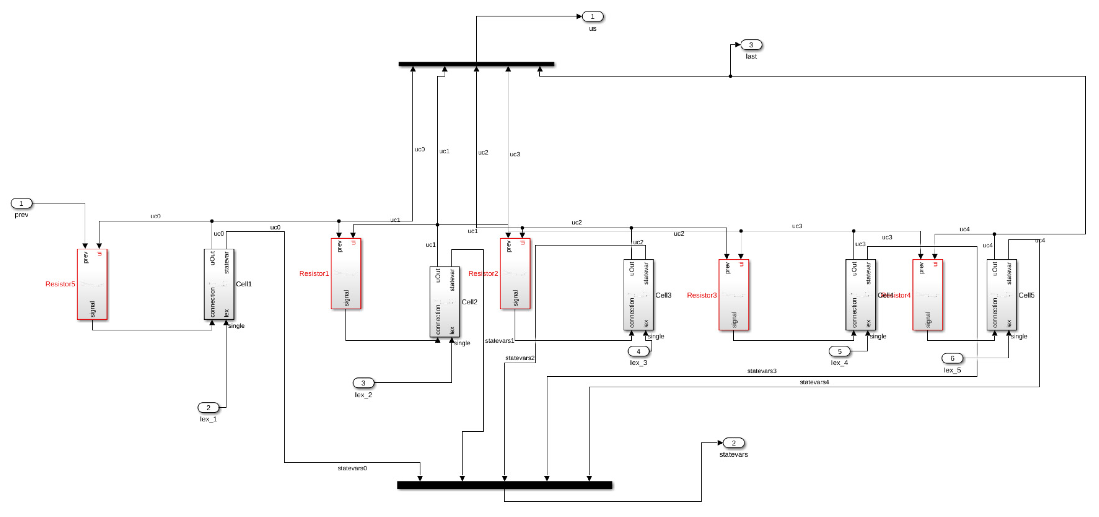
From the implementation point of view, we found Matlab^®Simulink very suitable for the development of rapid model prototypes. However, it is limited when it is necessary to handle large scale simulations. Furthermore, it was not possible to change the length of the cable/ring at runtime. Thus, we were not able to test the self-adapting properties described in the previous sections. In addition, the values of the variables at a certain time step cannot be updated using just the values of the previous step but rather all the values already computed in the current step. Furthermore, we found that the computational resources required to compile large HCA models with several cells were prohibitive (we could consider only models with a length of max. 3000 cells). Due to these restrictions, we could not implement the decreasing ring and the related Monte Carlo analysis in this environment. Nevertheless, as illustrated in the space-time plot shown in Figure 11b, we were able to induce electrical alternans with a trapped wave in a ring with a small number of cells by setting the value of the resistance to $2.0$.

We performed the same numerical experiments by using CPU-based and GPU-based implementations (see Figure 11d). Due to the negligible error between the results obtained using GPU and CPU, in Figure 11 we only provide the result obtained using CPU as representative. While Figure 11b,d look very similar, there is actually a small difference in the APD alternans profile. Specifically, the APD in Figure 11d, is longer than in Figure 11b.

If we observe the color representing the value of the variable u, we notice that the transition in Figure 11a is softer and shorter than in Figure 11c. This is due to the different mechanisms for updating the variables in Matlab^®Simulink previously discussed and that are not suitable to implement CA updating rules that depend on the values of the previous step.

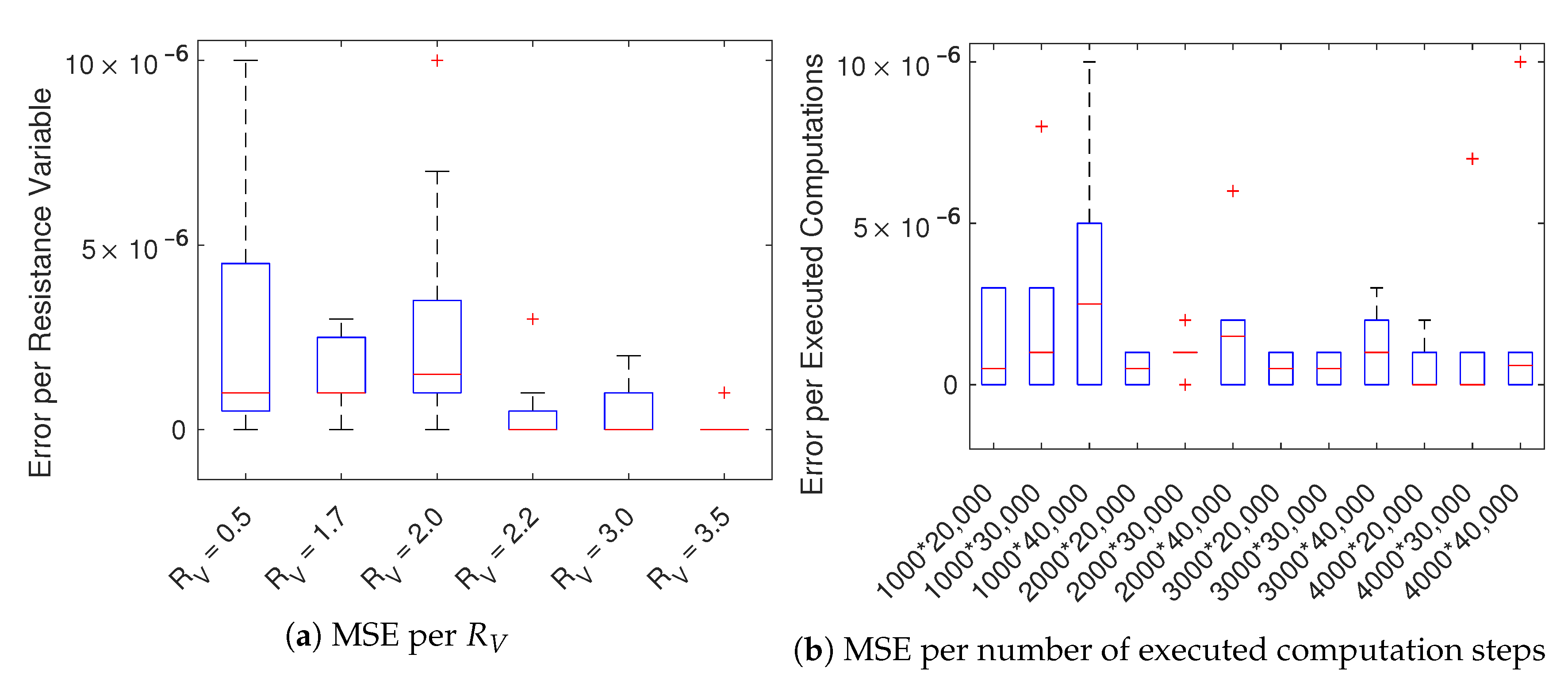
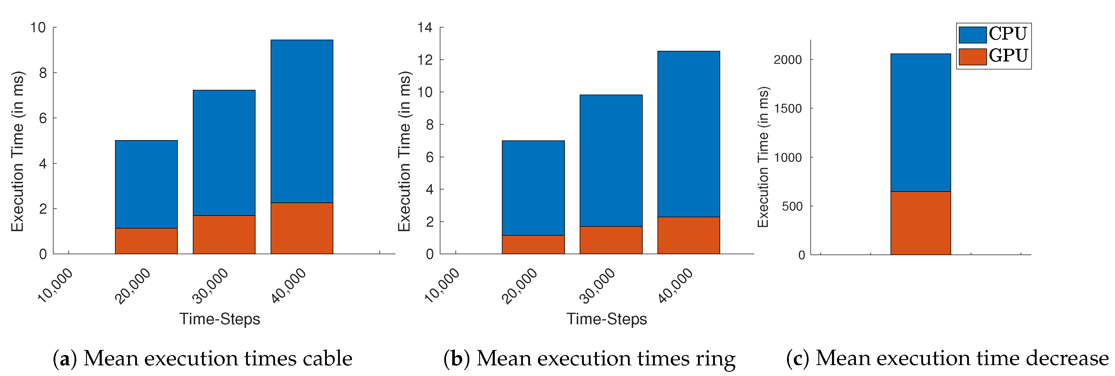
We, therefore, focused on the implementations using CPU (sequential) and GPU (parallel), producing instead results with a negligible difference (the average mean squared error is $1.3361\times {10}^{-6}$). As expected, the parallel GPU-based implementation benefits of the use of many-cores accelerating considerable the simulation. In Figure 5 we compute the average execution times for all used lengths and $R_V$. For simulations with a fixed number of time-steps, only the number of cells and time-steps increase the execution times.

The longest execution time measured was the decreasing ring simulation in both implementations, as we stop when no AP can be recovered. Still, the average execution time overall lengths and $R_V$ for this scenario using GPU is $1/4$ compared to the measured times using CPU, as shown in Figure 5c. Since this kind of analysis does not depend on a fixed number of time-steps, but it relies on the AP dynamics, the execution time for this scenario depends highly on the number of cells and the chosen value for the resistance $R_V$, shown in Table A4 and Table A5.

If we consider simulations with a fixed number of time-steps, the GPU implementation started to perform approximately 10× faster on average than the CPU-based implementation for simulations with more than 40,000 time-steps. If we consider the simulations with the highest number of required time-steps, this becomes more evident: the average measured execution time for simulating the ring with 40,000 time-steps and 2750 cells on GPU is ~2.60 ms while on the CPU required on average 21.60 ms. For the cable using these lengths and number of time-steps, the GPU implementation finishes consistently with an average of ~2.60 ms, while the CPU implementation required (less time than in the ring setting) within ~14.86 ms. In all implementations, we were able to control the CV with the free resistance variable.

Although it is possible to observe APD fluctuations at the beginning of the Monte Carlo simulations of shorter rings, the critical limit in length for the onset of the alternans is consistent in all ring sizes simulated using both CPU and GPU implementations. The occurrence of alternans depends only on the distribution of the resistance and thus on the resulting CV.

The observed decrease in the CV and the occurrence of APD fluctuations in inhomogeneous settings can be compared to the behavior observed in studies of ischemic cardiac tissue [59,60]. Even though we have slight inhomogeneities in the cell’s resistance, our analysis shows that the APD is stable until the length falls below a certain critical point when too many cells undergo large oscillations, thus a continuous propagation. Such a condition depends on the chosen initial number of cells and CV, as we could observe an early onset with both von Mises distributions that we have considered. Considering a CV of $380\mathsf{\mu }\mathrm{m}/\mathrm{ms}$, the obtained APD is similar to the results in [11] attained considering a regular body temperature of 37 °C. It is also similar to the original measurement data for epicardial cells referenced in [16].

5. Conclusions

We have presented an HCA modeling the cardiac cell-cell membrane resistance with a free variable.

We provide three different implementations comparing pros and cons: one using the Matlab^®Simulink graphical environment, a second implementation running on a CPU sequentially, and a third implementation running on a GPU in parallel. While Matlab^®Simulink provides a suitable environment for fast prototyping complex models is less efficient in handling simulation instances of large HCA models. The GPU-based implementation could handle instead larger instances accelerating considerably the simulation (in our experiments, we could observe 10× speed-up with respect to the CPU-based implementation) and indeed the overall analysis of the model.

We then study the cardiac behavior within a unidimensional domain considering inhomogeneous resistance by performing a Monte Carlo simulation. We show that our modeling approach can reproduce important and complex spatiotemporal properties such as self-adaptive properties and the onset of alternans, paving the ground for promising future applications.

In future work, we plan to extend our analysis from the one-dimensional cases to two and three spatial dimensions, including the possibility to use different cell types. We foresee to generalize the present study towards an efficient computation of ECG signals [61] simulating pathological conditions adapting critical parameters such as the free resistance variable and the ionic time constants. Additionally, we aim to apply our HCA computational approach in a more physiological context by implementing species-specific models [62,63,64,65] and investigating the underlying genetics [66] linked to cell-to-cell communications problems [67,68,69].

As mentioned in [58,70,71], the estimation of cardiac conductivity is still under investigation; therefore, we need to consider approaches to determine a more precise value for this parameter for future work. One strategy worth investigating is to use machine learning approaches or optimization algorithms such as the one described in [58] that map the free resistance variable to a specific conduction velocity. We also plan to improve our GPU-based implementation by combining our current approach with other optimizations described in other papers such as [34,72,73].

The use of other hardware accelerators, such as FPGAs that are becoming more and more employed to handle computational extensive problems in simulation [74,75] and graphic processing [76,77] represents a promising perspective.

References

1. Beeler, G.W.; Reuter, H. Reconstruction of the action potential of ventricular myocardial fibres. J. Physiol. 1977, 268, 177–210. [Google Scholar] [CrossRef]
2. Luo, C.H.; Rudy, Y. A model of the ventricular cardiac action potential. Depolarization, repolarization, and their interaction. Circ. Res. 1991, 68, 1501–1526. [Google Scholar] [CrossRef] [Green Version]
3. Karma, A. Electrical alternans and spiral wave breakup in cardiac tissue. Chaos 1994, 4, 461–472. [Google Scholar] [CrossRef]
4. Iyer, V.; Mazhari, R.; Winslow, R.L. A Computational Model of the Human Left-Ventricular Epicardial Myocyte. Biophys. J. 2004, 87, 1507–1525. [Google Scholar] [CrossRef] [Green Version]
5. Hodgkin, A.L.; Huxley, A.F. A quantitative description of membrane current and its application to conduction and excitation in nerve. J. Physiol. 1952, 117, 500–544. [Google Scholar] [CrossRef]
6. Noble, D. A modification of the Hodgkin—Huxley equations applicable to Purkinje fibre action and pacemaker potentials. J. Physiol. 1962, 160, 317–352. [Google Scholar] [CrossRef]
7. Noble, D. From the Hodgkin–Huxley axon to the virtual heart. J. Physiol. 2007, 580, 15–22. [Google Scholar] [CrossRef]
8. Dierckx, H.; Fenton, F.H.; Filippi, S.; Pumir, A.; Sridhar, S. Simulating normal and arrhythmic dynamics: From sub-cellular to tissue and organ level. Front. Phys. 2019, 7, 89. [Google Scholar] [CrossRef] [Green Version]
9. Bartocci, E.; Singh, R.; von Stein, F.B.; Amedome, A.; Caceres, A.J.; Castillo, J.; Closser, E.; Deards, G.; Goltsev, A.; Ines, R.S.; et al. Teaching cardiac electrophysiology modeling to undergraduate students: Laboratory exercises and GPU programming for the study of arrhythmias and spiral wave dynamics. Adv. Physiol. Educ. 2011, 35, 427–437. [Google Scholar] [CrossRef] [Green Version]
10. Gizzi, A.; Loppini, A.; Ruiz-Baier, R.; Ippolito, A.; Camassa, A.; La Camera, A.; Emmi, E.; Di Perna, L.; Garofalo, V.; Cherubini, C.; et al. Nonlinear diffusion and thermo-electric coupling in a two-variable model of cardiac action potential. Chaos Interdiscip. J. Nonlinear Sci. 2017, 27, 093919. [Google Scholar] [CrossRef] [Green Version]
11. Fenton, F.H.; Gizzi, A.; Cherubini, C.; Pomella, N.; Filippi, S. Role of temperature on nonlinear cardiac dynamics. Phys. Rev. E 2013, 87, 042717. [Google Scholar] [CrossRef] [Green Version]
12. Ruiz Baier, R.; Gizzi, A.; Loppini, A.; Cherubini, C.; Filippi, S. Modelling Thermo-Electro-Mechanical Effects in Orthotropic Cardiac Tissue. Commun. Comput. Phys. 2019, 27. [Google Scholar] [CrossRef] [Green Version]
13. Bini, D.; Cherubini, C.; Filippi, S. On vortices heating biological excitable media. Chaos Solitons Fractals 2009, 42, 2057–2066. [Google Scholar] [CrossRef]
14. Welsh, A.J.; Delgado, C.; Lee-Trimble, C.; Kaboudian, A.; Fenton, F.H. Simulating waves, chaos and synchronization with a microcontroller. Chaos Interdiscip. J. Nonlinear Sci. 2019, 29, 123104. [Google Scholar] [CrossRef]
15. Fenton, F.; Karma, A. Vortex dynamics in three-dimensional continuous myocardium with fiber rotation: Filament instability and fibrillation. Chaos Interdiscip. J. Nonlinear Sci. 1998, 8, 20–47. [Google Scholar] [CrossRef]
16. Bueno-Orovio, A.; Cherry, E.M.; Fenton, F.H. Minimal model for human ventricular action potentials in tissue. J. Theor. Biol. 2008, 253, 544–560. [Google Scholar] [CrossRef]
17. Bartocci, E.; Corradini, F.; Berardini, M.R.D.; Entcheva, E.; Grosu, R.; Smolka, S.A. Spatial Networks of Hybrid I/O Automata for Modeling Excitable Tissue. Electron. Notes Theor. Comput. Sci. 2008, 194, 51–67. [Google Scholar] [CrossRef] [Green Version]
18. Grosu, R.; Batt, G.; Fenton, F.H.; Glimm, J.; Guernic, C.L.; Smolka, S.A.; Bartocci, E. From Cardiac Cells to Genetic Regulatory Networks. In Proceedings of the CAV 2011: The 23rd International Conference on Computer Aided Verification, Snowbird, UT, USA, 14–20 July 2011; Springer: Berlin/Heidelberg, Germany, 2011; Volume 6806, pp. 396–411. [Google Scholar] [CrossRef] [Green Version]
19. Wolfram, S. Cellular automata as models of complexity. Nature 1984, 311, 419–424. [Google Scholar] [CrossRef]
20. Murray, J. Mathematical Biology II: Spatial Models and Biomedical Applications; Springer Nature: Berlin/Heidelberg, Germany, 2013. [Google Scholar] [CrossRef]
21. Neumann, J.; Burks, A.W. Theory of Self-Reproducing Automata; University of Illinois Press Urbana: Champaign, IL, USA, 1966; Volume 1102024. [Google Scholar] [CrossRef]
22. Amorim, R.M.; Campos, R.S.; Lobosco, M.; Jacob, C.; dos Santos, R.W. An electro-mechanical cardiac simulator based on cellular automata and mass-spring models. In Proceedings of the International Conference on Cellular Automata, Santorini, Greece, 24–27 September 2012; Springer: Berlin/Heidelberg, Germany, 2012; pp. 434–443. [Google Scholar] [CrossRef]
23. Lehotzky, D.; Zupanc, G.K. Cellular Automata Modeling of Stem-Cell-Driven Development of Tissue in the Nervous System. Dev. Neurobiol. 2019, 79, 497–517. [Google Scholar] [CrossRef]
24. Grosu, R.; Smolka, S.A.; Corradini, F.; Wasilewska, A.; Entcheva, E.; Bartocci, E. Learning and Detecting Emergent Behavior in Networks of Cardiac Myocytes. Commun. ACM 2009, 52, 97–105. [Google Scholar] [CrossRef] [Green Version]
25. Bartocci, E.; Corradini, F.; Di Berardini, M.; Entcheva, E.; Smolka, S.; Grosu, R. Modeling and simulation of cardiac tissue using hybrid I/O automata. Theor. Comput. Sci. 2009, 410, 3149–3165. [Google Scholar] [CrossRef] [Green Version]
26. Andalam, S.; Ramanna, H.; Malik, A.; Roop, P.; Patel, N.; Trew, M.L. Hybrid automata models of cardiac ventricular electrophysiology for real-time computational applications. In Proceedings of the 2016 38th Annual International Conference of the IEEE Engineering in Medicine and Biology Society (EMBC), Orlando, FL, USA, 16–20 August 2016; pp. 5595–5598. [Google Scholar] [CrossRef]
27. Ye, P.; Grosu, R.; Smolka, S.A.; Entcheva, E. Formal Analysis of Abnormal Excitation in Cardiac Tissue. In Proceedings of the CMSB 2008: The 6th International Conference on Computational Methods in Systems Biology, Rostock, Germany, 12–15 October 2008; Volume 5307, pp. 141–155. [Google Scholar] [CrossRef] [Green Version]
28. Bartocci, E.; Lió, P. Computational Modeling, Formal Analysis, and Tools for Systems Biology. PLoS Comput. Biol. 2016, 12, e1004591. [Google Scholar] [CrossRef] [Green Version]
29. Cytrynbaum, E.N.; MacKay, V.; Nahman-Lévesque, O.; Dobbs, M.; Bub, G.; Shrier, A.; Glass, L. Double-wave reentry in excitable media. Chaos Interdiscip. J. Nonlinear Sci. 2019, 29, 073103. [Google Scholar] [CrossRef]
30. Sigalas, C.; Cremer, M.; Bose, S.; Burton, R.A. Combining tissue engineering and optical imaging approaches to explore interactions along the neuro-cardiac axis. R. Soc. Open Sci. 2020. [Google Scholar] [CrossRef]
31. Bub, G.; Glass, L.; Publicover, N.G.; Shrier, A. Bursting calcium rotors in cultured cardiac myocyte monolayers. Proc. Natl. Acad. Sci. USA 1998, 95, 10283–10287. [Google Scholar] [CrossRef] [Green Version]
32. Bartocci, E.; Cherry, E.M.; Glimm, J.; Grosu, R.; Smolka, S.A.; Fenton, F.H. Toward real-time simulation of cardiac dynamics. In Proceedings of the 9th International Conference on Computational Methods in Systems Biology, Paris, France, 21–23 September 2011; ACM: New York, NY, USA, 2011; pp. 103–112. [Google Scholar] [CrossRef] [Green Version]
33. Mena, A.; Ferrero, J.M.; Matas, J.F.R. GPU accelerated solver for nonlinear reaction–diffusion systems. Application to the electrophysiology problem. Comput. Phys. Commun. 2015, 196, 280–289. [Google Scholar] [CrossRef]
34. Pires, C.W.S.; Vasconcellos, E.C.; Clua, E.W.G. GPU Memory Access Optimization for 2D Electrical Wave Propagation Through Cardiac Tissue and Karma Model Using Time and Space Blocking. In Proceedings of the International Conference on Computational Science and Its Applications, Cagliari, Italy, 1–4 July 2020; Springer: Berlin/Heidelberg, Germany, 2020; pp. 376–390. [Google Scholar] [CrossRef]
35. Xu, Q.; Zhu, D. FPGA-based Experimental Validations of Electrical Activities in Two Adjacent FitzHugh–Nagumo Neurons Coupled by Memristive Electromagnetic Induction. IETE Tech. Rev. 2020, 1–15. [Google Scholar] [CrossRef]
36. Adon, N.A.; Jabbar, M.H.; Mahmud, F. FPGA implementation for cardiac excitation-conduction simulation based on FitzHugh-Nagumo model. In Proceedings of the 5th International Conference on Biomedical Engineering in Vietnam, Ho Chi Minh City, Vietnam, 16–18 June 2014; Springer: Berlin/Heidelberg, Germany, 2015; pp. 117–120. [Google Scholar] [CrossRef]
37. Fenton, F.; Cherry, E. Models of cardiac cell. Scholarpedia 2008, 3, 1868. [Google Scholar] [CrossRef]
38. Hastings, H.M.; Fenton, F.H.; Evans, S.J.; Hotomaroglu, O.; Geetha, J.; Gittelson, K.; Nilson, J.; Garfinkel, A. Alternans and the onset of ventricular fibrillation. Phys. Rev. E 2000, 62, 4043–4048. [Google Scholar] [CrossRef] [Green Version]
39. Watanabe, M.; Fenton, F.; Evans, S.; Hastings, H.; Alain, K. Mechanisms for Discordant Alternans. J. Cardiovasc. Electrophysiol. 2003, 12, 196–206. [Google Scholar] [CrossRef]
40. Cherry, E.M.; Fenton, F.H. Suppression of alternans and conduction blocks despite steep APD restitution: Electrotonic, memory, and conduction velocity restitution effects. Am. J. Physiol.-Heart Circ. Physiol. 2004, 286, H2332–H2341. [Google Scholar] [CrossRef] [PubMed]
41. Gizzi, A.; Cherry, E.; Gilmour, R.F., Jr.; Luther, S.; Filippi, S.; Fenton, F.H. Effects of pacing site and stimulation history on alternans dynamics and the development of complex spatiotemporal patterns in cardiac tissue. Front. Physiol. 2013, 4, 71. [Google Scholar] [CrossRef] [PubMed] [Green Version]
42. Islam, M.A.; Cleaveland, R.; Fenton, F.H.; Grosu, R.; Jones, P.L.; Smolka, S.A. Probabilistic reachability for multi-parameter bifurcation analysis of cardiac alternans. Theor. Comput. Sci. 2019, 765, 158–169. [Google Scholar] [CrossRef]
43. Burger, M. Inverse problems in ion channel modelling. Inverse Probl. 2011, 27, 083001. [Google Scholar] [CrossRef]
44. Clerx, M.; Beattie, K.A.; Gavaghan, D.J.; Mirams, G.R. Four ways to fit an ion channel model. Biophys. J. 2019, 117, 2420–2437. [Google Scholar] [CrossRef]
45. Weinberg, S. Ephaptic coupling rescues conduction failure in weakly coupled cardiac tissue with voltage-gated gap junctions. Chaos 2017, 27, 093908. [Google Scholar] [CrossRef]
46. Courtemanche, M.; Glass, L.; Keener, J.P. Instabilities of a propagating pulse in a ring of excitable media. Phys. Rev. Lett. 1993, 70, 2182. [Google Scholar] [CrossRef]
47. Glass, L.; Josephson, M.E. Resetting and Annihilation of Reentrant Abnormally Rapid Heartbeat. Phys. Rev. Lett. 1995, 75, 2059–2062. [Google Scholar] [CrossRef]
48. Steinberg, B.E.; Glass, L.; Shrier, A.; Bub, G. The role of heterogeneities and intercellular coupling in wave propagation in cardiac tissue. Philos. Trans. R. Soc. Math. Phys. Eng. Sci. 2006, 364, 1299–1311. [Google Scholar] [CrossRef]
49. Fink, M.; Niederer, S.A.; Cherry, E.M.; Fenton, F.H.; Koivumäki, J.T.; Seemann, G.; Thul, R.; Zhang, H.; Sachse, F.B.; Beard, D.; et al. Cardiac cell modelling: Observations from the heart of the cardiac physiome project. Prog. Biophys. Mol. Biol. 2011, 104, 2–21. [Google Scholar] [CrossRef] [Green Version]
50. Patel, R.B.; Ng, J.; Reddy, V.; Chokshi, M.; Parikh, K.; Subacius, H.; Alsheikh-Ali, A.A.; Nguyen, T.; Link, M.S.; Goldberger, J.J.; et al. Early Repolarization Associated with Ventricular Arrhythmias in Patients with Chronic Coronary Artery Disease. Circ. Arrhythmia Electrophysiol. 2010, 3, 489–495. [Google Scholar] [CrossRef] [PubMed] [Green Version]
51. Kaboudian, A.; Cherry, E.M.; Fenton, F.H. Real-time interactive simulations of large-scale systems on personal computers and cell phones: Toward patient-specific heart modeling and other applications. Sci. Adv. 2019, 5. [Google Scholar] [CrossRef] [PubMed] [Green Version]
52. Klabunde, R. Cardiovascular Physiology Concepts; Lippincott Williams & Wilkins: Philadelphia, PA, USA, 2011. [Google Scholar]
53. Mines, G.R. On circulating excitations in heart muscles and their possible relation to tachycardia and fibrillation. Trans. R. Soc. Can. 2010, 1914, 43–52. [Google Scholar]
54. Rytand, D.A. The Circus Movement (Entrapped Circuit Wave) Hypothesis and Atrial Flutter. Ann. Intern. Med. 1966, 65, 125–159. [Google Scholar] [CrossRef] [PubMed]
55. Loppini, A.; Gizzi, A.; Ruiz-Baier, R.; Cherubini, C.; Fenton, F.H.; Filippi, S. Competing Mechanisms of Stress-Assisted Diffusivity and Stretch-Activated Currents in Cardiac Electromechanics. Front. Physiol. 2018, 9. [Google Scholar] [CrossRef]
56. Cherubini, C.; Filippi, S.; Gizzi, A.; Ruiz-Baier, R. A note on stress-driven anisotropic diffusion and its role in active deformable media. J. Theor. Biol. 2017, 430, 221–228. [Google Scholar] [CrossRef]
57. Loppini, A.; Gizzi, A.; Cherubini, C.; Cherry, E.M.; Fenton, F.H.; Filippi, S. Spatiotemporal correlation uncovers characteristic lengths in cardiac tissue. Phys. Rev. E 2019, 100, 020201. [Google Scholar] [CrossRef] [Green Version]
58. Barone, A.; Gizzi, A.; Fenton, F.; Filippi, S.; Veneziani, A. Experimental validation of a variational data assimilation procedure for estimating space-dependent cardiac conductivities. Comput. Methods Appl. Mech. Eng. 2020, 358, 112615. [Google Scholar] [CrossRef]
59. Gottwald, E.; Gottwald, M.; Dhein, S. Enhanced dispersion of epicardial activation–recovery intervals at sites of histological inhomogeneity during regional cardiac ischaemia and reperfusion. Heart 1998, 79, 474–480. [Google Scholar] [CrossRef]
60. Taggart, P.; Sutton, P.M.; Opthof, T.; Coronel, R.; Trimlett, R.; Pugsley, W.; Kallis, P. Inhomogeneous Transmural Conduction During Early Ischaemia in Patients with Coronary Artery Disease. J. Mol. Cell. Cardiol. 2000, 32, 621–630. [Google Scholar] [CrossRef]
61. McSharry, P.E.; Clifford, G.D.; Tarassenko, L.; Smith, L.A. A dynamical model for generating synthetic electrocardiogram signals. IEEE Trans. Biomed. Eng. 2003, 50, 289–294. [Google Scholar] [CrossRef] [PubMed] [Green Version]
62. Hund, T.J.; Rudy, Y. Rate Dependence and Regulation of Action Potential and Calcium Transient in a Canine Cardiac Ventricular Cell Model. Circulation 2004, 110, 3168–3174. [Google Scholar] [CrossRef] [PubMed] [Green Version]
63. Sarai, N.; Matsuoka, S.; Kuratomi, S.; Ono, K.; Noma, A. Role of Individual Ionic Current Systems in the SA Node Hypothesized by a Model Study. Jpn. J. Physiol. 2003, 53, 125–134. [Google Scholar] [CrossRef] [PubMed] [Green Version]
64. Mahajan, A.; Shiferaw, Y.; Sato, D.; Baher, A.; Olcese, R.; Xie, L.H.; Yang, M.J.; Chen, P.S.; Restrepo, J.G.; Karma, A.; et al. A Rabbit Ventricular Action Potential Model Replicating Cardiac Dynamics at Rapid Heart Rates. Biophys. J. 2008, 94, 392–410. [Google Scholar] [CrossRef] [PubMed] [Green Version]
65. Cherry, E.M.; Ehrlich, J.R.; Nattel, S.; Fenton, F.H. Pulmonary vein reentry—Properties and size matter: Insights from a computational analysis. Heart Rhythm 2007, 4, 1553–1562. [Google Scholar] [CrossRef] [PubMed]
66. Rice, J.J.; Wang, F.; Bers, D.M.; De Tombe, P.P. Approximate Model of Cooperative Activation and Crossbridge Cycling in Cardiac Muscle Using Ordinary Differential Equations. Biophys. J. 2008, 95, 2368–2390. [Google Scholar] [CrossRef] [PubMed] [Green Version]
67. Lenarda, P.; Gizzi, A.; Paggi, M. A modeling framework for electro-mechanical interaction between excitable deformable cells. Eur. J. Mech.-A/Solids 2018, 72, 374–392. [Google Scholar] [CrossRef] [Green Version]
68. McCain, M.L.; Lee, H.; Aratyn-Schaus, Y.; Kléber, A.G.; Parker, K.K. Cooperative coupling of cell-matrix and cell–cell adhesions in cardiac muscle. Proc. Natl. Acad. Sci. USA 2012, 109, 9881–9886. [Google Scholar] [CrossRef] [Green Version]
69. Rohr, S. Role of gap junctions in the propagation of the cardiac action potential. Cardiovasc. Res. 2004, 62, 309–322. [Google Scholar] [CrossRef]
70. Barone, A.; Fenton, F.; Veneziani, A. Numerical sensitivity analysis of a variational data assimilation procedure for cardiac conductivities. Chaos 2017, 27, 093930. [Google Scholar] [CrossRef]
71. Barone, A.; Michele G., C.; Alessio, G.; Simona, P.; Veneziani, A. Efficient estimation of cardiac conductivities: A proper generalized decomposition approach. J. Comput. Phys. 2020, 423, 109810. [Google Scholar] [CrossRef]
72. Campos, J.; Oliveira, R.; dos Santos, R.; Rocha, B. Lattice Boltzmann method for parallel simulations of cardiac electrophysiology using GPUs. J. Comput. Appl. Math. 2016, 295, 70–82, VIII Pan-American Workshop in Applied and Computational Mathematics. [Google Scholar] [CrossRef]
73. Arthurs, C.J.; Bishop, M.J.; Kay, D. Efficient simulation of cardiac electrical propagation using high-order finite elements II: Adaptive p-version. J. Comput. Phys. 2013, 253, 443–470. [Google Scholar] [CrossRef]
74. Yang, C.; Geng, T.; Wang, T.; Patel, R.; Xiong, Q.; Sanaullah, A.; Wu, C.; Sheng, J.; Lin, C.; Sachdeva, V.; et al. Fully integrated FPGA molecular dynamics simulations. In Proceedings of the International Conference for High Performance Computing, Networking, Storage and Analysis, Denver, CO, USA, 17–22 November 2019; pp. 1–31. [Google Scholar] [CrossRef] [Green Version]
75. Bakhteri, R.; Cheng, J.; Semmelhack, A. Design and Implementation of Cellular Automata on FPGA for Hardware Acceleration. Procedia Comput. Sci. 2020, 171, 1999–2007. [Google Scholar] [CrossRef]
76. Siddiqui, F.; Amiri, S.; Minhas, U.I.; Deng, T.; Woods, R.; Rafferty, K.; Crookes, D. FPGA-Based Processor Acceleration for Image Processing Applications. J. Imaging 2019, 5, 16. [Google Scholar] [CrossRef] [Green Version]
77. Georgis, G.; Lentaris, G.; Reisis, D. Acceleration techniques and evaluation on multi-core CPU, GPU and FPGA for image processing and super-resolution. J. Real-Time Image Process. 2019, 16, 1207–1234. [Google Scholar] [CrossRef] [Green Version]
Figure 1. Schematic propagation in a 4-cell-HCA with vanishing activation wave propagation.
Mathematics 09 00164 g001
Figure 2. 1D cell structures circuit schematic. Panel (a) sketches a cable and Panel (b) a ring with 3 cells each. Cells are represented as voltage source and the resistors in between represent the membrane resistance.
Mathematics 09 00164 g002
Figure 3. Schematic of GPU and CPU communication and memories. Left, memory interaction on a single execution grid created by a single kernel call, with N sketched (thread) blocks and multiple threads within the blocks on GPU. Right, CPU interface and legend.
Mathematics 09 00164 g003
Figure 4. Boxplots of the mean squared error E of the variable u among CPU and GPU solutions. Panel (a) are sampled per R V over increasing number of executed computations ( N T ) while panel (b) per number of executed computations ( N T ) over varying R V .
Mathematics 09 00164 g004
Figure 5. Mean execution times over all cable lengths and resistance values for GPU (orange) and CPU (blue). (a) Cable, (b) ring, and (c) decreasing ring structure.
Mathematics 09 00164 g005
Figure 6. CV (in μ m / ms ) in different sized cell rings with varying value for R V .
Mathematics 09 00164 g006
Figure 7. Von Mises distribution functions for R V spatial characterization.
Mathematics 09 00164 g007
Figure 8. APD bifurication diagrams of four sampled cells within the decreasing ring experiment. The original number of cells is 1000 (10 cm). Parameters of the used von Mises distribution μ = 1.55 , κ = 8 .
Mathematics 09 00164 g008
Figure 9. APD bifurication diagrams of two rings with 1750 cells (17.5 cm) and different von Mises distributions: (a) μ = 1.55, κ = 8; (b) μ = 1.98, κ = 10.
Mathematics 09 00164 g009
Figure 10. Bifurication diagrams of four sampled cells within the decreasing ring experiment. The original number of cells is 2500 (25 cm). von Mises Distribution parameters μ = 1.98 , κ = 10 .
Mathematics 09 00164 g010
Figure 11. Space-time diagram comparison. The x-axis indicates the simulation time (in ms), the y-axis the length (in mm). Colormaps refer to the voltage variable u.
Mathematics 09 00164 g011
Publisher’s Note: MDPI stays neutral with regard to jurisdictional claims in published maps and institutional affiliations.