Abstract
We consider a class of cooperative differential games with continuous updating making use of the Pontryagin maximum principle. It is assumed that at each moment, players have or use information about the game structure defined in a closed time interval of a fixed duration. Over time, information about the game structure will be updated. The subject of the current paper is to construct players’ cooperative strategies, their cooperative trajectory, the characteristic function, and the cooperative solution for this class of differential games with continuous updating, particularly by using Pontryagin’s maximum principle as the optimality conditions. In order to demonstrate this method’s novelty, we propose to compare cooperative strategies, trajectories, characteristic functions, and corresponding Shapley values for a classic (initial) differential game and a differential game with continuous updating. Our approach provides a means of more profound modeling of conflict controlled processes. In a particular example, we demonstrate that players’ behavior is braver at the beginning of the game with continuous updating because they lack the information for the whole game, and they are “intrinsically time-inconsistent”. In contrast, in the initial model, the players are more cautious, which implies they dare not emit too much pollution at first.
1. Introduction
Dynamic or differential games are an important subsection of game theory that investigates interactive decision-making over time. A differential game is when the evolution of the decision process takes place over a continuous time frame, and it generally involves a differential equation. Differential games provide an effective tool for studying a wide range of dynamic processes such as, for example, problems associated with controlling pollution where it is important to analyze the interactions between participants’ strategic behaviors and the dynamic evolution in the levels of pollutants that polluters release. In Carlson and Leitmann [1], a direct methodfor finding open-loop Nash equilibria for a class of differential n-player games is presented.
Cooperative optimization points to the possibility of socially optimal and individually rational solutions to decision-making problems involving strategic action over time. The approach to solving a static cooperative differential game is typically done using a two-step procedure. First, one determines the collective optimal solution and then payoffs are transferred and distributed by using one of the many accessible cooperative game solutions, such as core, Shapley value, nucleolus. In the dynamic cooperative game, it must be assured that, over time, all players will comply with the agreement. This will occur if each player’s profits in the cooperative situation at any intermediate moment dominate their non-cooperative profits. This property is known as time consistency and was introduced by Petrosjan (originally 1977) [2].
In order to derive equilibrium solutions, existing differential games often depend on the assumption of time-invariant game structures. However, the future is full of essentially unknown events. Therefore, it is necessary to consider that the information available to players about the future be limited. In the realm of dynamic updating, the Looking Forward Approach is used in game theory, and in differential games especially. The Looking Forward Approach solves the problem of modeling players’ behavior when the process information is dynamically updating. This means that the Looking Forward Approach does not use a target trajectory, but composes how a trajectory is to be used by players and how a cooperative payoff is to be allocated along that trajectory. The Looking Forward Approach was first presented in [3]. Afterward, the works in [4,5,6,7,8,9] were published.
In [10,11,12,13,14,15], a class of non-cooperative differential games with continuous updating is considered, and it is assumed that the updating process continues to develop over time. In the paper [10], the Hamilton–Jacobi–Bellman equations of the Nash equilibrium in the game with the continuous updating are derived. The work in [11] is devoted to the class of cooperative differential games with the transferable utility using Hamilton–Jacobi–Bellman equations, construction of characteristic function with continuous updating and several related theorems. Another result related to Hamilton–Jacobi–Bellman equations with continuous updating is devoted to the class of cooperative differential games with nontransferable utility [15]. The works in [13,14] are devoted to the class of linear-quadratic differential games with continuous updating. There the cooperative and non-cooperative cases are considered and corresponding solutions are obtained. In the paper [12], the explicit form of the Nash equilibrium for the differential game with continuous updating is derived by using the Pontryagin maximum principle. In this paper, the class of cooperative game models is examined and results concerning a cooperative setting such as the construction of the notion of cooperative strategies, the characteristic function, and cooperative solution for a class of games with continuous updating using Pontryagin maximum principle are presented. Theoretical results for three players are illustrated on a classic differential game model of pollution control presented in [16]. Another potentially important application of continuous updating approach is related to the class of inverse optimal control problems with continuous updating [17]. The approach can be used for human behavior modeling in engineering systems.
The class of differential games with dynamic and continuous updating has some similarities with Model Predictive Control (MPC) theory which is worked out within the framework of numerical optimal control in the books [18,19,20,21]. The current action of control is realized by solving a limited level of open-loop optimal control problem at each sampling moment in the MPC method. For linear systems, there is an explicit solution [22,23]. However, in general, the MPC approach needs to solve several optimization problems. Another series of related papers corresponding to the stable control category is [24,25,26,27], in which similar methods are considered for the linear-quadratic optimal control problem category. However, the goals of the current paper and the paper on continuous updating methods are different: when the information about the game process is continuous updated over time, the player’s behavior can be modeled. In [28,29], a similar issue is considered and the authors investigate repeated games with sliding planning horizons.
The paper is structured as follows. Section 2 starts with the initial differential game model and cooperative differential model. Section 3 demonstrates the knowledge of a differential game with continuous updating and a cooperative differential game with continuous updating by using the Pontryagin maximum principle method and obtains the definition of a characteristic function with continuous updating. It also presents the results of the theoretical portion. Section 4 gives an example of pollution control based on continuous updating. The conclusion is drawn in Section 5.
2. Initial Differential Game Model
2.1. Preliminary Knowledge
Consider the differential game starting with the initial position and evolving on time interval . The equations of the system’s dynamics have the form
where is a set of variables that characterizes the state of the dynamical system at any instant of time during the play of the game, , is the control of player i. We shall use the notation .
The existence, uniqueness, and continuability of solution for any admissible measurable controls was dealt with by Tolwinski, Haurie, and Leitmann [30]:
- is continuous.
- There exists a positive constant k such that
- , such thatfor all x and such that
- for any and setis a convex compact from .
The payoff of player i is then defined as
where , are the integrable functions, is the solution of the Cauchy problem (1) with fixed open-loop controls . The strategy profile is called admissible if the problem (1) has a unique and continuable solution.
Let us agree that in a differential game, a subgame is a “truncated” version of the whole game. A subgame is a game in its own right and a subgame starts out at time instant , after a particular history of actions . Denote such a subgame by . (A remark on this notation is in order. Let the state of the game be defined by the pair and denote by the subgame starting at date t with the state variable x; here, the model considered is of a finite horizon and we will have the terminal time T. If we take account of the infinite horizon, of course, one expects all corresponding value functions to depend on state and not on time.)
For each , we define a subgame by replacing the objective functional for player i and the system dynamics by
and
respectively. Therefore, is a differential game defined on the time interval with initial condition .
2.2. Cooperative Differential Game Model
We adopt a cooperative game methodology to solve the differential game model with transferable utility. The steps are as follows.
- Define the cooperative behavior or strategies and corresponding cooperative trajectory.
- Determine the computation of the characteristic function values.
- Allocate among players a total cooperative payoff, such as the allocation belongs to the kernel, the bargaining set, the stable set, the core, the Shapley value and the nucleolus (see, e.g., Osborne and Rubinstein [31] for an introduction to these concepts).
First of all, we introduce the notions of cooperative strategies for players and the corresponding trajectory . Strategies are called optimal strategies, i.e., a set of controls that maximizes the joint payoff of players:
Suppose that the maximum in (2) is achieved on the set of admissible strategies. If we substitute into Equation (1), we can get the cooperative trajectory .
Consequently, to determine the way to distribute the maximum total payoff among players, it is fundamental to define the concept of the characteristic function of the coalition . This characteristic function shows the strength of the coalition; remarkably, it allows us to take into account the players’ contributions to each coalition.
To define a cooperative game, a characteristic function must be introduced. We call , is a characteristic function for the initial differential game . Through a characteristic function we understand a map from the set of all possible coalitions:
which assigns to each coalition S the total payoff value which the players from S can guarantee when acting independently. An important property is the superadditivity of a characteristic function:
The question of constructing a characteristic function is one of the main questions in cooperative game theory. Originally, the value of the characteristic function was interpreted by von Neumann and Morgenstern (1944) as the maximum guaranteed payoff of coalition S that it can gain acting independently of other players [32]. Presently, it is known that there are various means of constructing characteristic functions in cooperative games, such as —c.f. [33], —c.f. [34], —c.f. [35], and —c.f. [36].
Similar to the above, for each , we define a cooperative subgame (The superscript “c” means “cooperative”) along the cooperative trajectory by replacing the objective functional for player i and the system dynamics by
and
respectively. Therefore, is a cooperative differential game defined on the time interval with initial condition .
In this paper, we will adopt the constructive approach proposed by Petrosjan L. and Zaccour G. [37] with respect to putting together a -characteristic function. denotes the strength of a coalition S for the subgame , it can be calculated in two stages: in the beginning, we are obliged to compute the Nash equilibrium strategies for all players , and second, we refrigerate the strategy for the players of , and the players of the coalition S seek to maximize their joint revenue on . Thus, the definition of the characteristic function is given:
Denote by the set of imputations in the game :
where is a value of characteristic function for coalition .
By represent any cooperative solution or subset of imputation set :
In fact, the two extensively used cooperative solutions are the Shapley value and the core. In the following, we will consider a specific cooperative solution referred to as the Shapley value [38]. The Shapley value selects a single imputation, an n-vector denoted , satisfying three axioms: fairness, which means similar players are treated equally; efficiency (); and linearity (a relatively technical axiom required to obtain uniqueness). The Shapley value is defined in a unique way and is particularly suitable for a range of applications.
The Shapley value in the game is a vector, such that
3. Differential Game with Continuous Updating
3.1. Preliminary Knowledge
In order to compose the corresponding differential game with continuous updating, we will apply the classic differential game with the specified duration of to the continuously updated differential game. Consider the family of games starting from the state x at an arbitrary time . Furthermore, assume that the evolution of the state of the game can be described by the ordinary differential equation
where is the derivative with respect to s, are the state variables of a game that initials from time t, and , indicates the control profile of the game that initials from time t at the instant time s.
For the game , the player’s payoff function has the following form,
where , are trajectory and strategy profile in the game .
The continuously updated differential games can be established in consonance with the following rules.
The instant time is continuously evolving, and appropriately, players continue to attain new information about the equations of motion and payment functions in the game .
The strategy vector in the continuously updated differential game is as follows,
where , are strategies in the game .
Determine the trajectory in the continuously updated differential game according to
where are strategies in the continuously updated differential game (6), and is the derivative with respect to t. We assume that the strategy in the continuously updated differential game achieved using (6) is either admissible, or that the uniqueness and continuity of the solution of problem (7) can be guaranteed. The existence, uniqueness, and continuity conditions of the open-loop Nash equilibrium for the continuously updated differential game have been mentioned previously.
There is the indispensable difference between a continuously updated differential game and a classic differential game with the specified duration . In the case of classic game, the players are conducted by payoffs that they will finally gain within the time interval ; but in the game with continuous updating, they orient themselves toward the expected payoffs (5) at each time instant , which are computed due to the information determined by the interval , or the information that they possess at the instant time t. The subgame of the initial game has the form , by using the same method we can define a family subgames of the differential game with continuous updating at each t as , where is the state at the instant time . We will define this next.
First, we introduce the dynamic of the state:
Therefore, the payoff function of player i in a subgame with continuous updating has the form
where satisfy (8) and , , are strategies in the subgame .
3.2. Cooperative Differential Game with Continuous Updating
In a cooperative setting, before starting the game, all players agree to behave jointly in an optimal way (cooperate).
3.2.1. The Approach to Define the Characteristic Function on the Interval
We introduce the notion of characteristic function , defined for each subgame , which , . Before introducing the characteristic function for the subgame , it should be mentioned that from the Equation (4), we can derive that depends on the initial point x. Therefore, we can replace by x in the previous statement, such as by using and to represent the subgame and the payoff function for each player i of the subgame, respectively. Thus, the characteristic function is given:
where , , , which we have already described in (4). Moreover, is the strategy profile for the players in the coalition S.
We assume that superadditivity conditions for the characteristic function are satisfied:
3.2.2. An Algorithm to Calculate Characteristic Function with Continuous Updating and the Shapley Value
The first three steps are to compute the necessary elements in order to define the characteristic function. In the next step, the Shapley value is computed.
Step 1: Optimizing the total payment of the grand coalition with continuous updating.
We shall refer to the cooperative differential game described above by , the duration of the game is . We believe that there are no inherent obstacles to cooperation between players, and their benefits can be transferred. More specifically, we assume that before the game actually starts, the players agree to cooperate in the game.
Definition 1.
Strategy profile is generalized open-loop cooperative strategies in a game with continuous updating if, for any fixed strategy profile, are open-loop cooperative strategies in game .
Using the generalized open-loop cooperative strategies, it seems possible to define the solution concept for a game model with continuous updating.
Definition 2.
Strategy profile are called open-loop cooperative strategies in a game with continuous updating when defined in the following way,
where has defined the above.
We would like to interpret that the “intrinsically time-inconsistent” of players as follows:
- in the moment t coincides with cooperative strategies in the game defined on the interval ,
- in the instant has to coincide with cooperative strategies in the game defined on the interval .
Trajectory that corresponds to open-loop cooperative strategies with continuous updating can be obtained from the system
Here, denotes a cooperative trajectory with continuous updating.
Let there exist a set of controls
such that
The solution of the system (11) corresponding to is called the corresponding generalized cooperative trajectory.
Theorem 1.
Let be continuously differentiable at , ,
be continuously differentiable on ,.
A set of strategies, , provides generalized open-loop cooperative strategies in a differential game with continuous updating to the problem in (11), if for any fixed , there exists a costate variable with so that the following relations are satisfied:
(1) , for ,
(2) , where , ,
(3) , where ,
.
Remark 1.
Let fix and consider game .
The motion equation is in the form
The payoff function of the grand coalition has the form
If , are the generalized open-loop cooperative strategies in the differential game with continuous updating; then, as stated in Definition 1, for every fixed , , is an open-loop cooperative strategy in game . Therefore, for any fixed , the conditions (1)–(3) of the theorem are satisfied as necessary conditions for cooperative strategies in open-loop strategies (see in [39]).
On the other hand, if for every , the Hamiltonian are concave in , then the conditions of the theorem are sufficient for a cooperative open-loop solution [40].
Then, for any fixed , we can obtain the generalized open-loop cooperative strategy and its corresponding state trajectory , . Using Definitions 1 and 2, we can obtain the cooperative strategies with continuous updating and corresponding cooperative trajectory with continuous updating , .
In order to get the characteristic function of the grand coalition in subgame , substituting and into the corresponding payoff function, denote as the function of the coalition N. The current-value maximized cooperative payoff can be expressed as
Step 2: Computation of the generalized open-loop Nash equilibrium with continuous updating.
The problem of a non-cooperative subgame along the cooperative trajectory with continuous updating can be stated as follows,
where .
In this setting, the current-value Hamiltonian function can be written as
where , . By using the Pontryagin maximum principle with continuous updating [12], we can get the open-loop Nash equilibrium , and the corresponding trajectory , . It is then easy to derive the characteristic function of a single-player coalition as follows, for each
Step 3: Compute the characteristic function for all remaining possible coalitions with continuous updating.
Here, we need to compute only the coalitions that contain more than one player and exclude a grand coalition. There will be subsets obtained in the following way. We will apply the -characteristic function so that players of S maximize their total payoff along the cooperative strategy with continuous updating , while the other players, those from , use generalized open-loop Nash-equilibrium strategies
Thus, we have a two-stage construction procedure for the characteristic function: (1) Find generalized open-loop Nash equilibrium strategies for all players , which we have found in the Step 2; (2) “Freeze” the Nash equilibrium strategies for players from , and, as for the player from the coalition S, maximize their total payoff over . In order to compute the value function of the subgame , ,, we present the following concept.
Definition 3.
A set of strategies , , provides a generalized open-loop optimal strategy for coalition in a subgame with continuous updating when it is the solution obtained by using the Pontryagin maximum principle of the following problem
The Hamiltonian function of the problem (14) has the form, (The uppercase letter “S” in the paper always denotes the coalition S, e.g., , , and :
Theorem 2.
Let
be continuously differentiable on , ,
be continuously differentiable on
A set of strategies, , provides a generalized open-loop optimal strategies of the coalition S in subgame with continuous updating to the problem (14) if there exists costate functions , where , , so that, for , , the following relations are satisfied:
(1) , , for ,
(2) , for , where
(3) , where , , .
Proof.
Follow the proof of Theorem 1. □
Therefore, the agents in the coalition S will adopt the generalized open-loop optimal control characterized in Theorem 2. Note that these controls are functions of fixed time and instant time .
An illustration of the characteristic function for the coalition is provided in the following way,
where is the trajectory at time instant when the players in coalition S use generalized open-loop optimal strategies , while players in use generalized open-loop Nash equilibrium that was already derived in Step 2.
For the characteristic function in the game model with continuous updating, first, suppose that the function , can be continuously differentiated by . Moreover, through can be integrated, the characteristic function in the game model with continuous updating is defined as follows.
Definition 4.
Function , , is a characteristic function of the differential game with continuous updating , if it is defined as the following integral,
where , , , defined on the interval is a characteristic function in game .
In (15), we assume that the intergal is taken with a finite time interval because in this case we can only claim that the values of the characteristic function with continuous updating are finite. Later on in the example model, we shall calculate the characteristic function and Shapley value using the final interval method. We assume that superadditivity conditions are satisfied:
Step 4: Compute the Shapley value based on the characteristic function with continuous updating.
Consider again the cooperative game model with continuous updating. If the players are allowed to form different coalitions consisting of a subset of all players . There are k players in the subset K. An imputation set of cooperative game is the set , which satisfies the conditions
A cooperative solution or the optimal principle is a non-empty subset of the imputation set . In particular, the Shapley value is an imputation whose components are defined as
where is the relative complement of i in K, the notion is defined by Definition 4 and is the profit of coalition K. Meanwhile, is the marginal contribution of player i to coalition K.
There are many other cooperative optimality principles, for example, the von Neumann–Morgenstern solution, N-core, and nucleus. In all cases they involve some subsets of the game imputation set.
4. A Cooperative Differential Game for Pollution Control
Let us consider the following game proposed by Long [41]. When countries are indexed by , we denote that . It is assumed that each player has an industrial production site and the production is proportional to the pollutant . Therefore, the player’s strategy is to decide the amount of pollutants emitted into the atmosphere.
4.1. Initial Game Model
Pollution accumulates over time. We denote by the stock of pollution at time t and assume that the countries “contribute” to the same stock of pollution. For simplicity, the evolution of stock is represented by the following linear equation:
where is a constant rate of decay, in other words, the absorption rate of pollution by nature.
In the following, we assume that the absorption coefficient is equal to zero:
Pollution is a “public bad” because it exerts adverse affects on health, quality of life, and productivity. We assume that these adverse effects can be represented by having x as an argument of the instantaneous social welfare function , with negative derivative:
In each country, aggregate social welfare is taken to be the integral of the instantaneous social welfare. Thus, the payoff of the player i can be formulated as follows,
For tractability, the function is often assumed to take the separable form:
where may be thought of as the utility of the benefit, and as the “disutility” caused by pollution. Following standard practice, we take it that is strictly concave and increasing in , and that is convex and increasing in x. The possibility that is linear is not ruled out.
We assume that the environmental damage cost of player i caused by the pollution stock is and the damage cost increases convexly. In the environmental economics literature, the typical assumption is that the production income function of player i can be expressed as a function of emissions, namely, , satisfying , where and are positive parameters. For the above benefit function to have a concave increase in emissions, we impose the restriction .
Suppose that the game is played in a cooperative scenario in which players have the opportunity to cooperate in order to achieve maximum total payoff:
To solve the optimization problem in (19) and (18), we invoke the Pontryagin maximum principle to characterize the solution as follows. Obviously, these are linear state games (These are games for which the system dynamics and the utility functions are polynomials of degree 1 with respect to the state variables and which satisfy a certain property (described below) concerning the interaction between control variables and state variables. We call this class of games linear state games.). This shows that these games have the property that their open-loop Nash equilibrium are Markov perfect. The class of linear state games has a very useful property. The linearity in the state variables together with the decoupled structure between the state variables and the control variables implies that the open-loop equilibrium is Markov perfect and that the value functions are linear in the state variables.
It is obvious to demonstrate that the optimal emissions control of player i for an initial differential game model is given by
To obtain the cooperative state trajectory for the initial differential game, it suffices to insert in (20) into the dynamics and to solve the differential equation to get
4.2. A Pollution Control Game Model with Continuous Updating
In the game , the dynamics of the total amount of pollution is described by
in which we assume that the absorption coefficient corresponding to the natural purification of the atmosphere is equal to zero.
The instantaneous payoff of player is defined as
Due to decontamination, each player is compelled to bear the cost. Therefore, the instantaneous utility of the player is equal to , where .
Thus the payoff of the player i is defined as
where is the control of the player i at the instant time , is the pollution accumulation at the same time s.
Therefore, the payoff function of the player i in the subgame with continuous updating is given by
where , , and are both the trajectory and strategies in game . The dynamics of the state is given by
Step 1: Optimizing the total payment of the grand coalition with continuous updating.
Consider the game in a cooperative form. This means that all players will work together to maximize their total payoff. We seek the optimal profile of strategies such that .
The optimization problem is as follows,
In order to deal with the problem (24), we use the classical Pontryagin maximum principle. The corresponding Hamiltonian is
The first order partial derivatives w.r.t. ’s are
and the Hessian matrix is negative definite, all at once, we can conclude that the Hamiltonian is concave w.r.t. . Here, we obtain the cooperative strategies:
Considering the Pontryagin’s maximum principle, when dealing with the costate variable
if we set , so, we can get . Finally, the form of the cooperative strategies is
and from (22) we get the optimal (cooperative) trajectory:
where , , .
According to the procedure (10), we construct open-loop optimal cooperative strategies with continuous updating:
After substituting into the differential Equation (18), we can arrive at the optimal cooperative trajectory with continuous updating:
The results of the comparison of the cooperative strategies, corresponding trajectories between initial differential game model and the differential game with continuous updating obtained are graphically shown in Figure 1 and Figure 2.
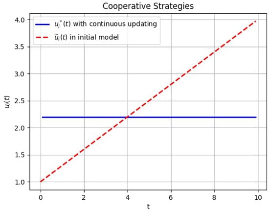
Figure 1.
Cooperative strategies in the initial game (red line) and cooperative strategies with continuous updating (blue line).
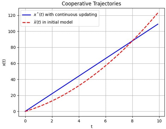
Figure 2.
Cooperative trajectory in the initial game (red line) and cooperative trajectory with continuous updating (blue line).
From Figure 1 we can see that the optimal control with continuous updating is more stable than the optimal control in the initial game model. We can also see that, from the time , the optimal control in the initial game is greater than it with continuous updating, which means players should increase the pollution emissions into the atmosphere in the initial differential game model, a harmful result. This occurs because in the initial game model, players have the whole information of the game on the interval , players are more cautious, and they dare not emit too much pollution at first. However, in real life, it is impossible to have the information for the whole time interval. Therefore, we consider the game with continuous updating, at each time instant t, players have the information only on . In the case of continuous updating, the players are brave enough to emit more pollution because of lacking the information for the whole game.
We can see from Figure 2 that, starting from to , the pollution accumulation in the initial game model is less than the model with continuous updating. Because in the initial game model, players are more knowledgeable, they know the information from the whole time interval, which leads to lower pollution accumulation because the players are cautious. Starting from time , pollution with continuous updating is less than pollution in the initial game because the knowledge for players in the model with continuous updating is close to the initial game model as time goes on. Using the continuous updating method can help us to make our modeling more consistent with the actual situation.
Next, for a given subgame of a differential game with continuous updating , the characteristic function for the grand coalition N is given by , which can be represented as
where satisfies (26) with , satisfies (25). Therefore, we can get the value function of the grand coalition N
where , has been defined above and . Note that in (29), represents the cooperative pollution with continuous updating at the time t.
For our problem, we can also use the dynamic programming method based on the Hamilton–Jacobi–Bellman equation. It is straightforward to verify the Bellman function of the form , and we get the same result as Pontryagin maximum principle.
Step 2: The computation of the generalized open-loop Nash equilibrium with continuous updating.
The Hamiltonian for each player is
its first-order partial derivatives w.r.t. ’s are
and the Hessian matrix is the negative definite whence we conclude that the Hamiltonian is concave w.r.t. . We obtain optimal controls
As for the subgame start at time instant , we can easily derive the corresponding trajectory (for the Nash equilibrium case) of subgame along the cooperative trajectory, in other words is
The maximum of the payoff for each player in the subgame starting from the time instant s and the state has the form
Step 3: The computation of the characteristic function for all remaining possible coalitions in differential games with continuous updating.
It is possible to calculate the controls and the corresponding value functions for different coalitions. Nonetheless, the form will depend on how we define their respective optimal control problems.
Let us build up the characteristic function hinged on the approach of —c.f. The characteristic function of coalition S is calculated in two stages: the first stage is already done (we have already found the Nash equilibrium strategies for each player in Step 2); at the second stage, it is assumed that the remaining players carry out their Nash optimal strategies although the players from coalition S explore to make their joint payoff maximal. Consider the case of S-coalition. It seems constructive to perform calculations in detail. The respective Hamiltonian for the coalition S is
where . Note that we substituted by which was found earlier.
The optimal strategies of players in coalition S are , which satisfies
The differential equation for is which is solved to ensure that . Eventually, we get . We substitute the obtained expression for into , and then get
where . We see that the player out of coalition S implements their optimal strategy while the left out players adhere to their Nash equilibrium.
In the next step, we integrate (23) start from the point to get :
is the trajectory in the subgame of the game starting at time instant s at , when players from coalition S use strategies , and players from coalition use . If we consider the case taken along the cooperative trajectory, then we can substitute the we have already obtained in (26) to get the state variable that depends on .
The respective value of the characteristic function is
According to Definition 4, the characteristic function of a differential game with continuous updating has the following form,
Check the superadditivity condition (16) for constructed characteristic function
. It turns out that for any and , let , the following holds,
Thus, the -characteristic function is a superadditive function without any additional conditions applied to the parameters of the model.
In the following figure, we will compare the characteristic function for the grand coalition N between the initial game model and a differential game with continuous updating.
Figure 3 demonstrates the reason accounting for why the value of a characteristic function in the initial model is greater than that of continuous updating is that the complexity of the information within a continuous updating setting can reduce the effectiveness of the coalition. It should be noted that the continuous updating case is more realistic. We can conclude that the payoff of the coalition decreases because, as time goes on, pollution accumulates in the air. The player’s payoff depends on levels of pollution and payoff decreases as pollution increases. It should also be noted that the coalition’s effectiveness decreases in the initial game model at a faster rate than it does with continuous updating.
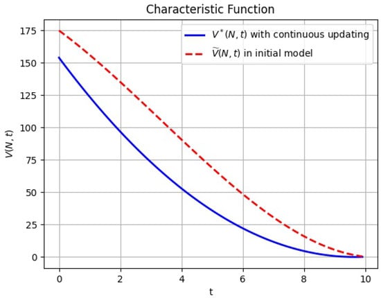
Figure 3.
The value of the characteristic function of a coalition N in the initial game (red line) and the value of the characteristic function of a coalition N with continuous updating (blue line).
Step 4: Compute the Shapley value based on the characteristic function with continuous updating.
Any of the known principles of optimality can be applied to find a cooperative solution. First of all, the notion (Here we should note that ) represents the interaction of cost among players. Now, consider the cooperative solution of a differential game with continuous updating. According to procedure (17), we construct the Shapley value for any with continuous updating using the characteristic function with continuous updating of the auxiliary subgame and get
The graphic representation of the Shapley value for subgames with continuous updating and the initial game model along the optimal cooperative trajectory is demonstrated in Figure 4.
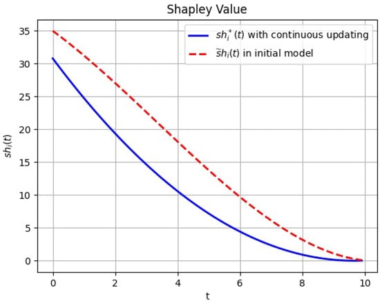
Figure 4.
The Shapley value of player i in the initial game (red line) and the Shapley value with continuous updating (blue line).
Figure 4 shows that if we consider the problem in a more realistic case (continuous updating), a player with continuous updating can get less allocation from the coalition than they get from the initial game model. This is based on the fact that, at an early stage, the pollution emitted into the atmosphere is more than in the initial game model, and in the latter stage the pollution with continuous updating is less than in the initial game model. Thus, starting with , players get more in the initial game model, but in the same period, they all get 0 in the end. This shows that as pollution intensifies the benefits countries receive from its attendant production gradually decrease.
5. Conclusions
In this paper, we presented the detailed consideration of a cooperative differential game model with continuous updating based on Pontryagin maximum principle, where the decision-maker updates his/her behavior based on the new information available which arises from a shifting time horizon. The characteristic function with continuous updating obtained by using the Pontryagin maximum principle for the cooperative case is constructed. The results show that the -characteristic function computed for the game is superadditive and does not have any other restrictions on the model’s parameters. The concept of the Shapley value as a cooperative solution with continuous updating is demonstrated in an analytic form for pollution control problems. Ultimately, considering the example of n-player pollution control, optimal strategies, the corresponding trajectory, the characteristic function, and the Shapley value with continuous updating are conceived for the proposed application and graphically compared for their effectiveness. We showed simulation results that show the applicability of the approach.
The practical significance of the work is determined by the fact that the real life conflict controlled processes evolve continuously in time and the players usually are not or cannot use full information about it. Therefore, it is important to introduce the type of differential games with information updating to the field of game theory. Another important practical contribution of the continuous updating approach is the creation of a class of inverse optimal control problems with continuous updating [17]. Problems that can be used to analyze a profile of the human in the human-machine type of engineering systems. The results are illustrated on the model of a driver assistance system and are applied to the real driving data from the simulator located in the Institute of Control Systems, Karlsruhe Institute of Technology. Our method can provide more in-depth modeling of human engineering systems.
Author Contributions
Conceptualization, J.Z.; Data curation, A.T.; Formal analysis, A.T.; Funding acquisition, O.P.; Investigation, O.P.; Methodology, J.Z.; Project administration, H.G.; Resources, H.G.; Software, J.Z.; Supervision, O.P. and H.G.; Validation, A.T.; Visualization, H.G.; Writing—original draft, J.Z.; Writing—review and editing, O.P. All authors have read and agreed to the published version of the manuscript.
Funding
This work is supported by Postdoctoral International Exchange Program of China and funded by the Russian Foundation for Basic Research (RFBR) according to the Grant No. 18-00-00727 (18-00-00725), and the National Natural Science Foundation of China (Grant No. 71571108).
Institutional Review Board Statement
Not applicable.
Informed Consent Statement
Not applicable.
Data Availability Statement
Not applicable.
Acknowledgments
The corresponding author would like to acknowledge the support from the China-Russia Operations Research and Management Cooperation Research Center, that is an association between Qingdao University and St. Petersburg State University.
Conflicts of Interest
The authors declare no conflict of interest.
References
- Carlson, D.A.; Leitmann, G. An Extension of the Coordinate Transformation Method for Open-Loop Nash Equilibria. J. Optim. Theory Appl. 2004, 123, 27–47. [Google Scholar] [CrossRef]
- Petrosjan, L. Agreeable Solutions in Differential Games. Int. J. Math. Game Theory Algebra 1997, 3, 165–177. [Google Scholar]
- Petrosian, O.L. Looking Forward Approach in Cooperative Differential Games. Int. Game Theory Rev. 2016, 18, 1–20. [Google Scholar]
- Petrosian, O.L. Looking Forward Approach in Cooperative Differential Games with infinite-horizon. Vestnik St.-Peterbg. Univ. Ser. 2016, 4, 18–30. [Google Scholar] [CrossRef]
- Petrosian, O.L.; Barabanov, A.E. Looking Forward Approach in Cooperative Differential Games with Uncertain-Stochastic Dynamics. J. Optim. Theory Appl. 2017, 172, 328–347. [Google Scholar] [CrossRef]
- Gromova, E.; Petrosian, O.L. Control of information horizon for cooperative differential game of pollution control. In Proceedings of the International Conference Stability and Oscillations of Nonlinear Control Systems, Moscow, Russia, 1–3 June 2016. [Google Scholar]
- Petrosian, O.L. About the Looking Forward Approach in Cooperative Differential Games with Transferable Utility. In Static and Dynamic Game Theory: Foundations and Applications; Springer: Berlin/Heidelberg, Germany, 2019. [Google Scholar]
- Petrosian, O.L.; Nastych, M.; Volf, D. Non-cooperative Differential Game Model of Oil Market with Looking Forward Approach. In Frontiers of Dynamic Games; Birkhäuser: Cham, Switzerland, 2018; pp. 189–202. [Google Scholar]
- Petrosian, O.L.; Shi, L.; Li, Y.; Gao, H. Moving Information Horizon Approach for Dynamic Game Models. Mathematics 2019, 7, 1239. [Google Scholar] [CrossRef]
- Petrosian, O.L.; Tur, A. Hamilton-Jacobi-Bellman Equations for Non-cooperative Differential Games with Continuous Updating. Commun. Comput. Inform. Sci. 2019, 1090, 178–191. [Google Scholar]
- Petrosian, O.L.; Tur, A.; Wang, Z. Cooperative differential games with continuous updating using Hamilton–Jacobi–Bellman equation. Optim. Methods Softw. 2020, 1275, 256–270. [Google Scholar] [CrossRef]
- Petrosian, O.L.; Tur, A.; Zhou, J. Pontryagin’s Maximum Principle for Non-cooperative Differential Games with Continuous Updating. Commu. Comput. Inform. Sci. 2020, 1275, 256–270. [Google Scholar]
- Kuchkarov, I.; Petrosian, O.L. On class of linear quadratic non-cooperative differential games with continuous updating. Lect. Notes Comput. Sci. 2019, 11548, 635–650. [Google Scholar]
- Kuchkarov, I.; Petrosian, O.L. Open-Loop Based Strategies for Autonomous Linear Quadratic Game Models with Continuous Updating. Lect. Notes Comput. Sci. 2020, 12095, 212–230. [Google Scholar]
- Wang, Z.; Petrosian, O.L. On class of non-transferable utility cooperative differential games with continuous updating. J. Dyn. Games 2020, 7, 291–2302. [Google Scholar] [CrossRef]
- Gromova, E. The Shapley Value as a Sustainable Cooperative Solution in Differential Games of Three Players. In Recent Advances in Game Theory and Applications; Petrosyan, L., Mazalov, V., Eds.; Springer: Petrozavodsk, Russia, 2015; pp. 67–89. [Google Scholar]
- Petrosian, O.; Inga, J.; Kuchkarov, I.; Flad, M.; Hohmann, S. Optimal Control and Inverse Optimal Control with Continuous Updating for Human Behavior Modeling (to be published). IFAC-PapersOnLine 2020, 7, 291–2302. [Google Scholar]
- Goodwin, G.; Seron, M.; Dona, J. Constrained Control and Estimation: An Optimisation Approach; Springer: Berlin/Heidelberg, Germany, 2005. [Google Scholar]
- Kwon, W.; Han, S. Receding Horizon Control: Model Predictive Control for State Models; Springer: Berlin/Heidelberg, Germany, 2005. [Google Scholar]
- Rawlings, J.; Mayne, D. Model Predictive Control: Theory and Design; Nob Hill Publishing, LLC.: Madison, WI, USA, 2009. [Google Scholar]
- Wang, L. Model Predictive Control System Design and Implementation Using MATLAB; Springer: Berlin/Heidelberg, Germany, 2005. [Google Scholar]
- Bemporad, A.; Morari, M.; Dua, V.; Pistikopoulos, E. The explicit linear quadratic regulator for constrained systems. Automatica 2002, 38, 3–20. [Google Scholar] [CrossRef]
- Hempel, A.; Goulart, P.; Lygeross, J. Inverse Parametric Optimization With an Application to Hybrid System Control. IEEE Trans. Automat. Control 2015, 60, 1064–1069. [Google Scholar] [CrossRef]
- Kwon, W.; Bruckstein, A.; Kailath, T. Stabilizing state-feedback design via the moving horizon method. In Proceedings of the 21st IEEE Conference on Decision and Control, Orlando, FL, USA, 8–10 December 1982; Volume 21, pp. 234–239. [Google Scholar]
- Kwon, W.; Pearson, A. A modified quadratic cost problem and feedback stabilization of a linear system. IEEE Trans. Automat. Control 1977, 22, 838–842. [Google Scholar] [CrossRef]
- Mayne, D.; Michalska, H. Receding horizon control of nonlinear systems. IEEE Trans. Automat. Control 1990, 35, 814–824. [Google Scholar] [CrossRef]
- Shaw, L. Nonlinear control of linear multivariable systems via state-dependent feedback gains. IEEE Trans. Automat. Control 1979, 24, 108–112. [Google Scholar] [CrossRef]
- Vasin, A.A.; Divtsova, A.G. Game-theoretic model of agreement on limitation of transboundary atmospheric pollution. Matematicheskaya Teoriya Igr Prilozheniya 2017, 9, 27–44. [Google Scholar]
- Vasin, A.A.; Divtsova, A.G. The repeated game modelling an agreement on protection of the environment. In Proceedings of the VIII Moscow International Conference on Operations Research (ORM2018), Omsk, Russia, 8–14 July 2018; Volume 1, pp. 261–263. [Google Scholar]
- Tolwinski, B.; Haurie, A.; Leitmann, G. Cooperative equilibria in differential games. J. Math. Anal. Appl. 1986, 119, 182–202. [Google Scholar] [CrossRef]
- Muthoo, A.; Osborne, M.J.; Rubinstein, A. A Course in Game Theory. Economica 1996, 63, 164–165. [Google Scholar] [CrossRef]
- Von Neumann, J.; Morgenstern, O. Theory of Games and Economic Behavior, 1st ed.; Princeton University Press: Princeton, NJ, USA, 1944. [Google Scholar]
- Von Neumann, J.; Morgenstern, O. The characteristic function. In Theory of Games and Economic Behavior, 2nd ed.; Princeton University Press: Princeton, NJ, USA, 1947; pp. 238–242. [Google Scholar]
- Reddy, P.V.; Zaccour, G. A friendly computable characteristic function. Math. Soc. Sci. 2016, 82, 18–25. [Google Scholar] [CrossRef]
- Gromova, E.; Petrosjan, L. On an approach to constructing a characteristic function in cooperative differential games. Automat. Remote Control 2017, 78, 1680–1692. [Google Scholar] [CrossRef]
- Chander, P.; Tulkens, H. The core of an economy with multilateral environmental externalities. Int. J. Game Theory 1997, 26, 379–401. [Google Scholar] [CrossRef]
- Petrosjan, L.; Zaccour, G. Time-consistent Shapley value allocation of pollution cost reduction. J. Econom. Dyn. Control 2003, 27, 381–398. [Google Scholar] [CrossRef]
- Shapley, L.S. A value for n-persons games. Ann. Math. Stud. 1953, 28, 307–318. [Google Scholar]
- Başar, T. Dynamic Noncooperative Game Theory, 2nd ed.; SIAM: Philadelphia, PA, USA, 1999; Volume 23. [Google Scholar]
- Leitmann, G.; Schmitendorf, W. Some Sufficiency Conditions for Pareto-Optimal Control. J. Dyn. Syst. Meas. Control 1973, 95, 356–361. [Google Scholar] [CrossRef]
- Long, N.V. Pollution control: A differential game approach. Ann. Operat. Res. 1992, 37, 283–296. [Google Scholar] [CrossRef]
Publisher’s Note: MDPI stays neutral with regard to jurisdictional claims in published maps and institutional affiliations. |
© 2021 by the authors. Licensee MDPI, Basel, Switzerland. This article is an open access article distributed under the terms and conditions of the Creative Commons Attribution (CC BY) license (http://creativecommons.org/licenses/by/4.0/).