Hybrid Assembly Path Planning for Complex Products by Reusing a Priori Data

Abstract

Assembly path planning (APP) for complex products is challenging due to the large number of parts and intricate coupling requirements. A hybrid assembly path planning method is proposed herein that reuses a priori paths to improve the efficiency and success ratio. The assembly path is initially segmented to improve its reusability. Subsequently, the planned assembly paths are employed as a priori paths to establish an a priori tree, which is expanded according to the bounding sphere of the part to create the a priori space for path searching. Three rapidly exploring random tree (RRT)-based algorithms are studied for path planning based on a priori path reuse. The RRT* algorithm establishes the new path exploration tree in the early planning stage when there is no a priori path to reuse. The static RRT* (S-RRT*) and dynamic RRT* (D-RRT*) algorithms form the connection between the exploration tree and the a priori tree with a pair of connection points after the extension of the exploration tree to a priori space. The difference between the two algorithms is that the S-RRT* algorithm directly reuses an a priori path and obtains a new path through static backtracking from the endpoint to the starting point. However, the D-RRT* algorithm further extends the exploration tree via the dynamic window approach to avoid collision between an a priori path and obstacles. The algorithm subsequently obtains a new path through dynamic and non-continuous backtracking from the endpoint to the starting point. A hybrid process combining the RRT*, S-RRT*, and D-RRT* algorithms is designed to plan the assembly path for complex products in several cases. The performances of these algorithms are compared, and simulations indicate that the S-RRT* and D-RRT* algorithms are significantly superior to the RRT* algorithm in terms of the efficiency and success ratio of APP. Therefore, hybrid path planning combining the three algorithms is helpful to improving the assembly path planning of complex products.

1. Introduction

Assembly is a crucial step to realizing the full functions of a product by constructing a complete structure, which becomes increasingly difficult with an increasing number of parts that make up the product [1,2,3,4,5]. Digital modelling and virtual assembly have been widely studied to solve this problem [6,7,8,9]. Assembly planning is an integral part of virtual assembly [10,11,12,13], which primarily includes assembly sequence planning (ASP), assembly line balancing (ALB), and assembly path planning (APP) [14,15,16,17,18,19].

APP consumes considerable time when there is a significant number of parts. Thus, some methods have been researched to improve its efficiency [20]. APP finds collision-free short paths from the initial location to the final position [20,21], which is similar to path planning for robots, vehicles, and drones, among other technologies [22,23,24,25,26,27]. Hassan et al. proposed a novel near-optimum APP algorithm based on the particle swarm optimization approach to solve the obstacle-free APP process in a 3D haptic-assisted environment [28]. Wei et al. proposed a centroidal Voronoi tessellation (CVT) for the intelligent control of self-assembly path planning of swarm robots [29]. Masehian et al. presented a new simple greedy heuristic method to solve the assembly sequence and path planning problem; the method tries to locally minimize geometric interference between parts being assembled along the main directions in each iteration, and it employs a sampling-based stochastic path planner to arrange short paths for parts while avoiding workspace obstacles [20]. Morato et al. presented a technique that combines motion planning and part interaction clusters based on multiple rapidly exploring random trees to improve the generation of assembly precedence constraints [30]. These studies are beneficial for improving the efficiency of path planning. However, most of the APP methods mentioned above involve a large amount of repeated computation, leading to low planning efficiency and high costs when generating the assembly path through all parts.

In these studies, the rapidly exploring random tree (RRT) is a typical random sampling algorithm in path planning which explores free space by generating leaf nodes randomly and uniformly to expand a tree structure. A collision-free path is obtained by backtracking from the leaf node to the parent node in sequence when a leaf node reaches the target area [30,31]. The randomness of the sampling points makes it difficult to obtain the optimal path even if the number of sampling points is sufficient. Therefore, the rapidly exploring random tree star (RRT*) algorithm is one algorithm that has been proposed to improve the RRT algorithm, making the path cost lower by improving the nearest point selection strategy [23,32]. However, the RRT* algorithm cannot obtain a low-cost assembly path in a short time, or even a valid assembly path, when the number of sampling points is small.

In assembly planning, the final positions of the assembled parts are in close proximity, although their initial positions are different. Hence, most of the assembly paths overlap or partially overlap, meaning that parts of these paths are repeatedly planned. Therefore, finding and reusing the planned paths is a feasible way to reduce repeated planning and improve planning efficiency [33,34]. The difference in initial part positions in the assembly presents a challenge for the direct reuse of the planned paths as a whole. Accordingly, the assembly paths must be segmented for effective reuse. Therefore, a hybrid path planning method based on the improved RRT* algorithm is proposed in this paper to plan the motion segments as paths with different starting points and the same target point by reusing the planned paths.

The rest of this paper is organized as follows. The establishment of the configuration space for path planning is introduced in Section 2. In Section 3, the static RRT* (S-RRT*) and dynamic RRT* (D-RRT*) algorithms are proposed, and the hybrid path planning method based on the improved RRT* algorithm is illustrated in detail. A case study is provided in Section 4 to compare and analyze the RRT*, S-RRT*, and D-RRT* algorithms. Section 5 concludes the paper.

2. Establishment of the Configuration Space for Path Planning

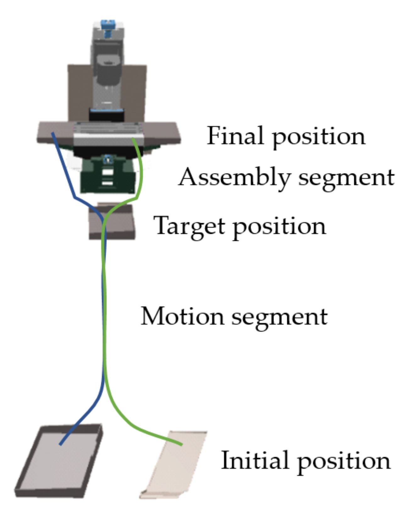
2.1. Segmentation of the Assembly Path

A position near the product assembly is defined as the target position. All the parts are moved from their initial positions to the target position and then assembled in the final positions. Therefore, an assembly path is divided into two segments: a motion segment from the initial position to the target position and an assembly segment from the target position to the final position, as shown in Figure 1.

The motion segment is arranged by reusing the planned path, and the assembly segment is directly planned. Combining the planning results of the two segments reduces repeated planning of the same or similar paths and improves the success ratio.

2.2. Part Shrinkage and Obstacle Expansion

There are many parts and obstacles in the assembly space of a complex product, which leads to high-complexity collision detection. Consequently, the assembly space is typically mapped to a configuration space for unified modelling before path planning. However, a substantial number of components with different shapes and sizes makes path planning a sizeable task if a new configuration space is created for each part. Therefore, the configuration space must be constructed reasonably and efficiently to support reusable path planning.

In path planning based on collision detection, a part is typically described with a bounding volume. The circumscribed sphere of a part is selected as its bounding sphere to simplify the description and calculation. In the equivalent transformation from the assembly space to the configuration space, the part shrinks according to the radius of its bounding sphere. All obstacle outlines are correspondingly expanded with the same radius (see Figure 2). In this way, path planning for a part in the assembly space is transformed into finding a noninterference path in the configuration space.

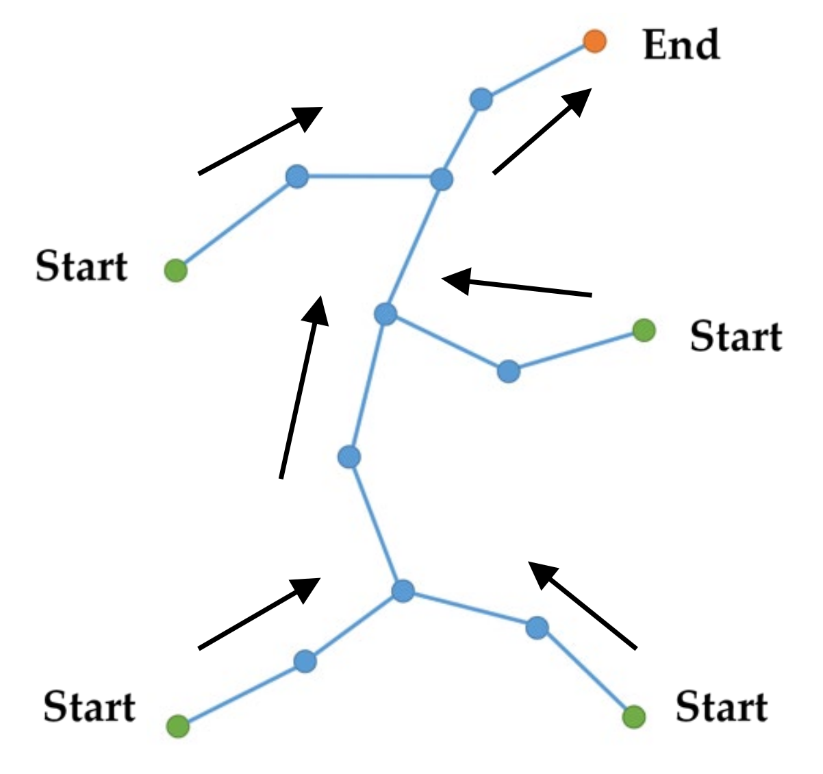
2.3. Establishment of the a Priori Path and a Priori Tree

An a priori path P_prior is a planned assembly path for a part, which is expressed as a linked list as shown in Equation (1):

P_prior = {p₁, p₂, …, p_i, …, p_n},

(1)

where each p_i is a node of the a priori path, and p₁ and p_n are the start and end nodes corresponding to the part’s initial position and target position, respectively.

A priori paths with different start nodes and the same end node form an a priori tree, where the leaf node is the start node of each path, the root node is the end node of all paths, and a branch from the leaf node to the root node is an a priori path, as shown in Figure 3. The reuse of an a priori path can be transformed into the search for an appropriate node of the a priori tree.

A node on the a priori tree may belong to different paths, and the number of such paths reflects its “importance”, which is defined as the weight of the node. The weight increases as the number of paths increases. The weight w_i of node p_i is defined as

w_i = n_i/n,

(2)

where n_i is the number of a priori paths crossing node p_i, and n is the total number of a priori paths. As shown in Equation (2), when the number of a priori paths crossing node p_i becomes bigger, the weight of node p_i also becomes bigger, which means that node p_i becomes more “important” among all the a priori paths.

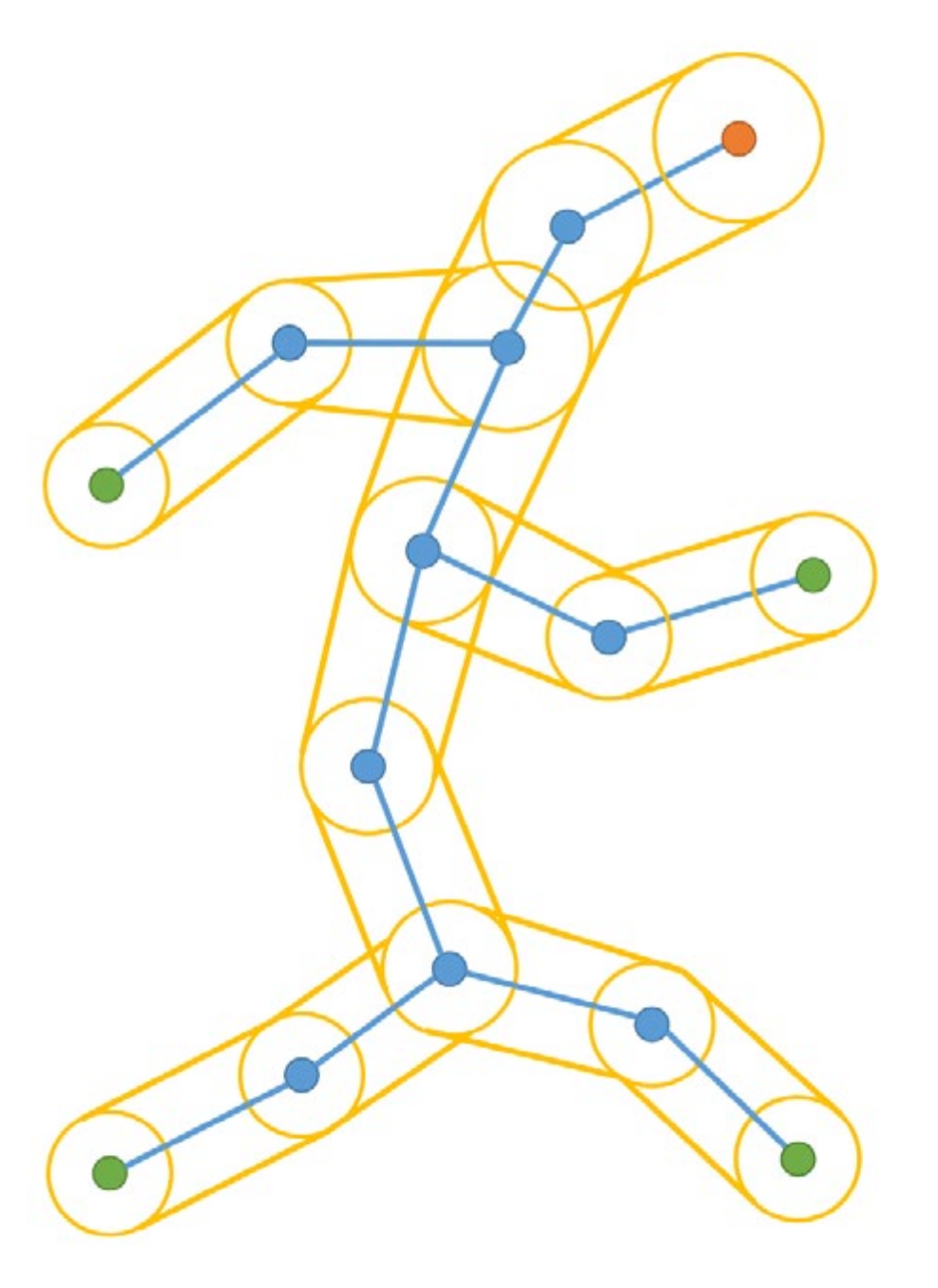
2.4. Expansion of the a Priori Space

The path planning algorithm based on random sampling extends the path by generating random points in the configuration space. If the a priori tree is only described using its nodes, the probability that the sampling points generated randomly coincide with the nodes is notably small, which makes finding and reusing the planned paths challenging. To solve this problem, the a priori tree is converted to an a priori space by expanding its nodes and branches, improving the reusability of the a priori paths.

Since the weight of a node expresses its “importance”, the expansion radius r_i of node p_i is positively related to its weight; that is,

r_i = d · w_i,

(3)

where d is the minimum distance between the nodes of the a priori path. According to Equation (3), when the weight of a node increases, this means that the number of a priori paths crossing node p_i increases, the radius of node p_i is greater, and the part of the a priori space of this node is larger.

Node p_i is expanded by constructing a circle with p_i as the center and r_i as the radius. External common tangents of every two adjacent circles are connected in turn. Figure 4 displays the space composed of all circles and common external tangents, which is the a priori space expanded from the a priori tree.

3. Algorithms for Path Reuse

The RRT algorithm is widely used in path planning; it randomly generates sampling points in the configuration space based on a tree structure and explores the configuration space according to the given steps. In theory, any point in the configuration space can be reached through the nodes of the tree in a specific sequence. Therefore, the RRT algorithm was used as the basis of the algorithms studied in this paper.

• RRT* algorithm for new path planning

It is difficult for the RRT algorithm to find the optimal path due to the randomness of the sampling points. As a result, the RRT* algorithm was proposed to lower the path cost by improving the nearest point selection strategy [31] of the RRT algorithm. The basic process of the RRT* algorithm is consistent with that of the RRT algorithm, and the main improvement is the strategy of adding new nodes and branches to the exploration tree.

In the early stage of APP, the RRT* algorithm is adopted because there is no a priori path to be reused. The key steps of the RRT* algorithm are as follows:

Step 1:

Point p_rand is randomly generated in the configuration space C.

Step 2:

Node p_near closest to p_rand is selected from the exploration tree with a connecting line, and a point on this line with a distance s (extension step of the exploration tree) from p_near is subsequently taken as a new leaf node, p_new.

Step 3:

The nearest node set ps_near is constructed with the nodes of the exploration tree in a certain range centered on p_new.

Step 4:

Node p_min is found as the parent of p_new by traversing ps_near, through which p_new is connected to the exploration tree with the minimum path cost.

Step 5:

p_new and p_min are added to the node set, and the branch connecting them is added to the branch set.

Compared to the RRT algorithm, it is similarly difficult for the RRT* algorithm to plan an assembly path with lower cost in a short time due to the excessive calculations.

2.

S-RRT* algorithm for static reuse of a priori paths

In the assembly of a new part, if there is an assembled part whose bounding sphere is not smaller than that of the new part, its configuration space can be utilized for path planning of the new part without any modification. Therefore, the path of the part can be directly reused as an a priori path to improve the planning efficiency. An S-RRT* algorithm (an improved RRT* algorithm statically reusing the a priori paths) is proposed in this case.

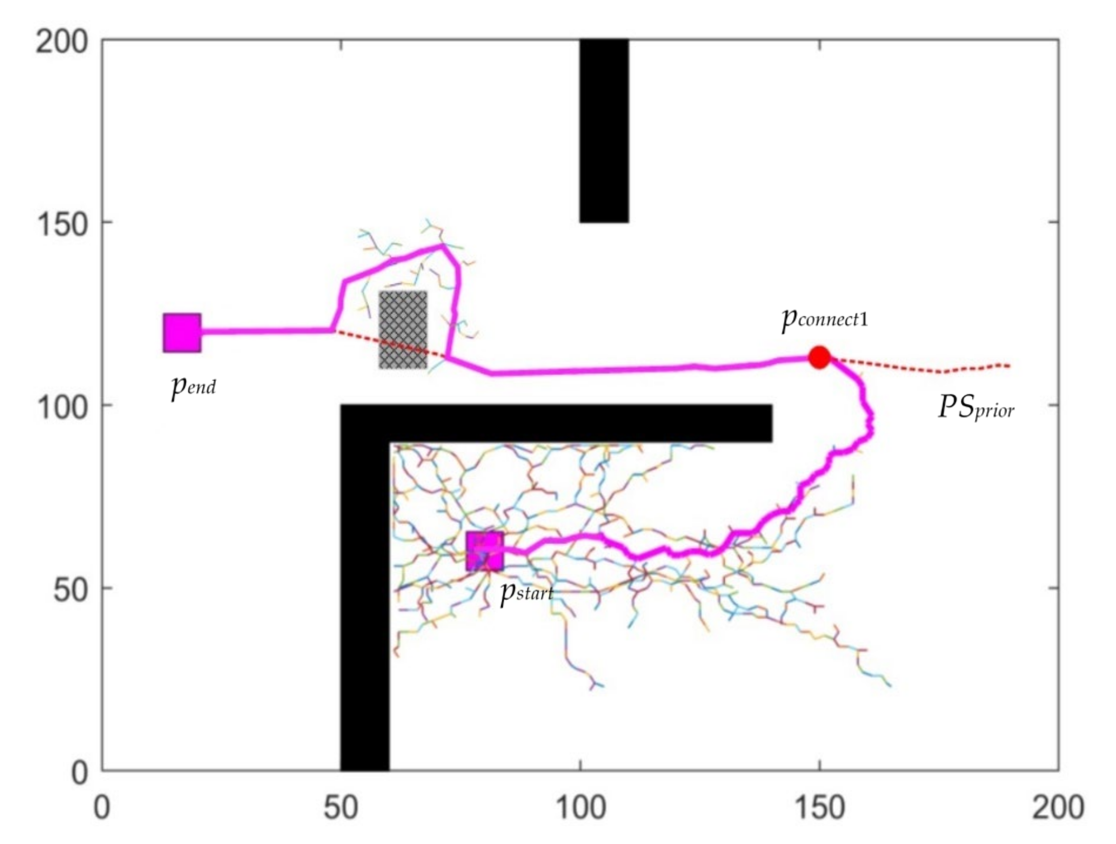
The main improvement of the S-RRT* algorithm is reusing the a priori paths after the exploration tree T_explore is extended to the a priori space C_prior. The S-RRT* algorithm aside from this reuse is consistent with the RRT* algorithm. The main steps of the S-RRT* algorithm are as follows:

Step 1:

A new leaf node p_new is generated on the line that connects the random point p_rand and its nearest node p_near, with a distance of s (expansion step) from p_near.

Step 2:

p_new is checked to confirm whether it is in the obstacle space C_obstacle. If so, the algorithm returns to Step 1; otherwise, the algorithm continues to the next step.

Step 3:

p_new is checked to verify whether it is in C_prior. If so, the exploration tree has been extended to the a priori space, and the algorithm goes to the next step; otherwise, the algorithm returns to Step 1.

Step 4:

Two nodes p_connect1 and p_connect2 are selected from the a priori tree T_prior and the exploration tree T_explore, respectively, according to p_new to connect the two trees.

Step 5:

The new branch E_new connecting p_connect1 and p_connect2 is added to T_explore, and a new path p_new is planned by backtracking from the end node p_end to the start node p_start and added to the a priori path set PS_prior.

Step 6:

After sampling N times, the cost of each new path in PS_prior is calculated, and the path with the lowest cost P_min is selected as the final path.

The pseudo-code of the S-RRT* algorithm is shown in Algorithm 1.

Algorithm 1 The static rapidly exploring random tree star (S-RRT*) algorithm.

Input: Cplan, Cobstacle, Cprior, pstart, pend, S, N, Tprior, Texplore

Result: A path Pmin with the minimum cost from pstart to pend

Texplore.init ();

PSprior.init ();

for n = 1 to N do

{

prand←Sample (Cplan);

pnear←Near (prand, Texplore);

pnew←Steer (prand, pnear, S);

if CollisionFree(Cobstacle, pnew) then

{

Pnear←Near (xnew, Texplore);

pmin←SelectParentNode (Pnear, pnear, pnew);

Texplore.AddEdge (Edge (xmin, pnew));

Texplore.Rewire();

if InPriorSpace (Cprior, pnew) then

{

pconnect1, pconnect2←ConnectNode (Texplore, Tprior, pnew);

Enew.AddEdge (pconnect1, pconnect2);

pnew←PathBacktrack (Texplore, Tprior, pconnect1, pconnect2)

PSprior.AddPath (pnew);

}

}

}

Pmin←MinCostPath (PSprior);

return Pmin;

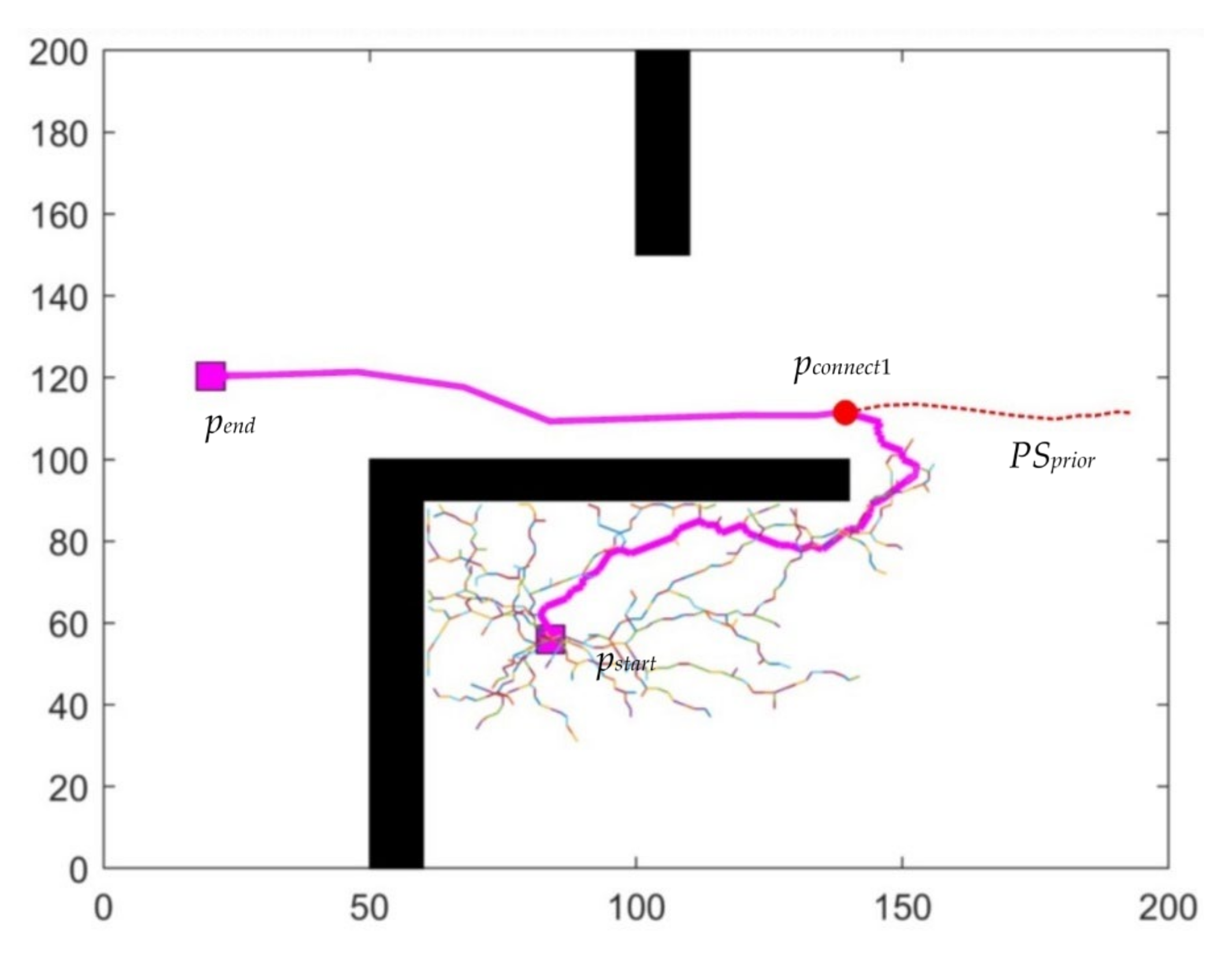
A path planned using the S-RRT* algorithm is shown in Figure 5. In this figure, a new assembly path is established, the part of the a priori path from p_connect1 to p_end is reused, and the path from p_start through p_connect1 to p_end is the final path generated by the S-RRT* algorithm. Compared with the RRT* algorithm, the S-RRT* algorithm generates a path with fewer sampling times by reusing the a priori path, which helps to improve the efficiency and success ratio of APP for complex products.

3.

D-RRT* algorithm for dynamic reuse of a priori paths

When assembling a new part, if the bounding sphere of the assembled part is smaller than that of the new part, its configuration space cannot be used for path planning of the new part. This is because the expansion of the new part’s obstacles is more extensive than that of the assembled part. The more formidable obstacles may interfere with the a priori path and lead to the failure of path planning using the S-RRT* algorithm. Therefore, a D-RRT* algorithm (an improved RRT* algorithm dynamically reusing the a priori path) is proposed to solve this problem. The main improvement of the D-RRT* algorithm is the utilization of the dynamic window approach [32] and further extension of the exploration tree to avoid interference between the a priori path and the obstacles after the connection node pair is found. The a priori path is reused non-continuously through dynamic backtracking to obtain the new path. The main steps of the dynamic backtracking of the a priori path are as follows:

Step 1:

Two connection nodes p_connect1 and p_connect2 are selected from the a priori tree T_prior and the exploration tree T_explore, respectively, as for the S-RRT* algorithm.

Step 2:

p_connect1 and its parent node p_parent are connected with a line to check whether the line interferes with obstacles. If there is no interference, p_parent is added to the new path, and the algorithm goes to Step 4; otherwise, the algorithm proceeds to Step 3.

Step 3:

The local path from p_connect1 to p_parent is planned and added to the new path.

Step 4:

p_connect1 and p_parent are updated with p_parent and its parent node, respectively, which expands the exploration tree along the a priori path.

Step 5:

p_connect2 is checked to determine whether it is the end node. If the end node is identified, a new path P_new is planned by backtracking from the end node p_end to the start node p_start; otherwise, the algorithm returns to Step 2.

The pseudo-code of the dynamic backtracking of the a priori path is shown in Algorithm 2.

Algorithm 2 Dynamic backtracking of the a priori path.

Input: Tprior, Texplore, pconnect1, pconnect2, Cobstacle, S

Result: A path Pnew without collision from pconnect1 to pconnect2

DynamicBacktracking(Tprior, Texplore, pconnect1, pconnect2, Cobstacle, S) {

pcurrent←pconnect1;

pparent←pcurrent.parentNodeInPriorTree ();

for j = 1 to N do {

if CollisionFree (Creusable, Cobstacle, pcurrent, pparent) then{

Pprior.addNode (pcurrent, pparent);

Pprior.addEdge (Edge (pcurrent, pparent));

}

else{

Plocal←LocalPath (pcurrent, pparent);

Pprior←addLocalPath (Plocal);

}

pcurrent←pparent;

pparent←pparent. parentNodeInPriorTree ();

if pparent = pconnect2 then {

return Pprior;

}

}

}

A path planned using the D-RRT* algorithm is shown in Figure 6. There is an obstacle in Figure 6 that did not appear in Figure 5, which occurs in the part of the a priori path from p_connect1 to p_end, and the D-RRT* algorithm can establish new assembly paths in this situation. Thus, a new assembly path was generated by D-RRT* from p_start through p_connect1 to p_end. The D-RRT* algorithm avoids obstacles by using dynamic backtracking and local path planning, which helps efficiently obtain an optimal assembly path without additional interference.

4.

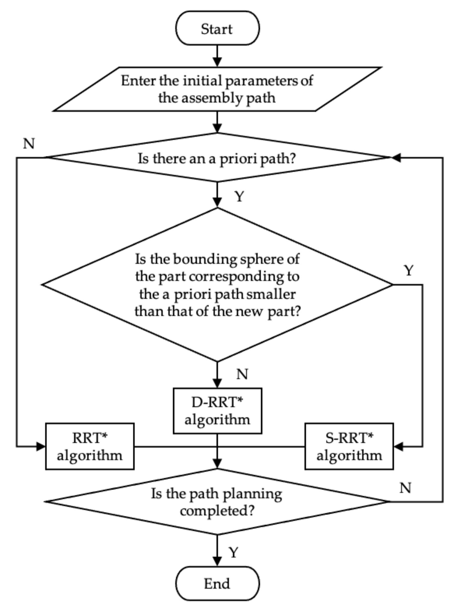
Hybrid process of the three algorithms

Using the three abovementioned algorithms, a hybrid process based on a priori path reuse was designed for assembly path planning, as presented in Figure 7.

4. Comparison and Analysis

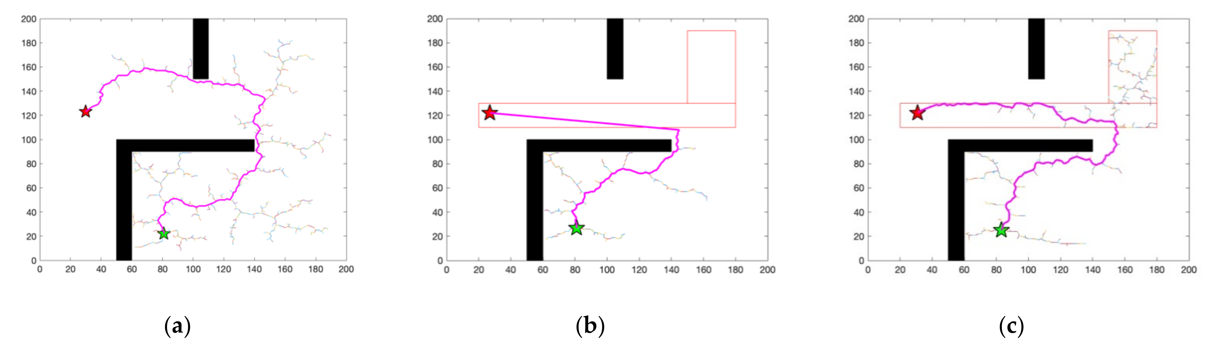
To analyze the performance of the RRT*, S-RRT*, and D-RRT* algorithms in the same case, a comparison is provided in this section. D-RRT* can also be applied in a situation in which there is no obstacle in the prior path, since it is an algorithm based on S-RRT* which can establish new path plans in the presence of obstacles, illustrated in detail in Section 3. Thus, a suitable case must be prepared to test the performance and make comparisons for the three algorithms. Assuming some a priori paths in the configuration space, the three algorithms mentioned above were used to plan the assembly path from the same starting point to the same endpoint, and one of the results is shown in Figure 8. Information relating to Figure 8 is presented in

Table 1. Information relating to Figure 8.

	Figure 8a	Figure 8b	Figure 8c
Max number of iterations	2000	2000	2000
Distance to the target threshold	5	5	5
Goal of probability	0.05	0.05	0.05
Step size	2	2	2
Path distance	314	128	286
Number of iterations	1104	330	1805
Number of tree branches	730	206	486

.

The randomness of sampling points in the three algorithms leads to large differences in the results of path planning, even with the same start and end points. Therefore, each algorithm was executed 100 times, and the averages of the minimum number of sampling points, the path length, and the running time of the three algorithms were compared, as illustrated in

Table 2. Comparison of the three algorithms in path planning with the same starting point.

Algorithm	Minimum Number of Sampling Points	Path Length	Running Time (s)
RRT*	1104	384	1.26
S-RRT*	330	248	0.356
D-RRT*	407	256	0.432

.

Table 2 demonstrates that the minimum numbers of sampling points for the S-RRT* algorithm and the D-RRT* algorithm were only 1/4 and 1/3 that for the RRT* algorithm, respectively, and their path length and running time were also less than those of the RRT* algorithm. The performance of the D-RRT* algorithm means that it is not as useful as the S-RRT* algorithm due to the additional sampling strategy.

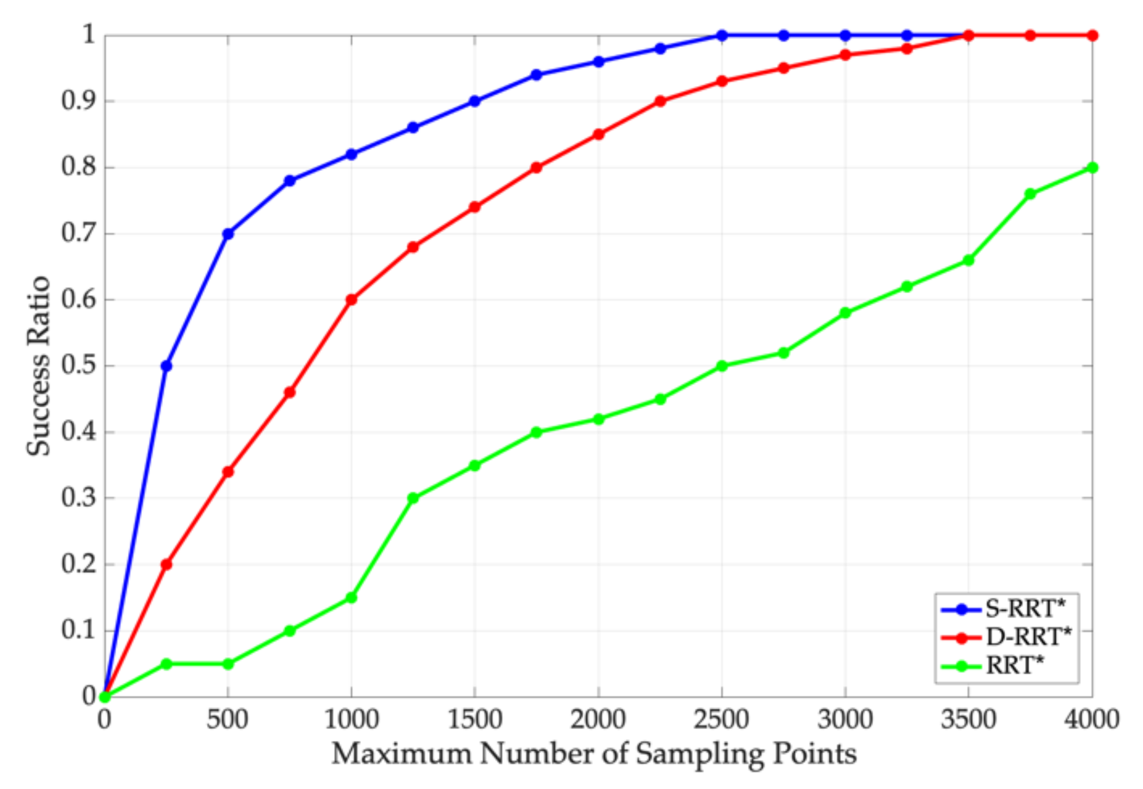
Considering that the start position of each part of a complex product is different in the assembly space, 50 starting points were randomly generated in the configuration space for the path planning simulation. The RRT*, S-RRT*, and D-RRT* algorithms were used to plan the assembly path for each starting point with different maximum numbers of sampling points. The number of successfully planned paths was used to calculate the path planning success ratio for multiple starting positions with the specified maximum number of sampling points, as shown in

Table 3. Comparison of the success ratios of path planning with the three algorithms.

Maximum Number of Sampling Points	Success Ratio of S-RRT* Algorithm	Success Ratio of D-RRT* Algorithm	Success Ratio of RRT* Algorithm
0	0.00	0.00	0.00
250	0.50	0.20	0.05
500	0.70	0.34	0.05
750	0.78	0.46	0.10
1000	0.82	0.60	0.15
1250	0.86	0.68	0.30
1500	0.90	0.74	0.35
1750	0.94	0.80	0.40
2000	0.96	0.85	0.42
2250	0.98	0.90	0.45
2500	1.00	0.93	0.50
2750	1.00	0.95	0.52
3000	1.00	0.97	0.58
3250	1.00	0.98	0.62
3500	1.00	1.00	0.66
3750	1.00	1.00	0.76
4000	1.00	1.00	0.80

.

Table 3 confirms that as the maximum number of sampling points increased, the success ratios of the three algorithms also increased. When the maximum number of sampling points was small, the success ratios of the S-RRT* algorithm and the D-RRT* algorithm were considerably greater than those of the RRT* algorithm. The success ratios of these three algorithms are also shown in Figure 9.

The minimum numbers of sampling points and the total running times of the three algorithms are specified in

Table 4. Comparison of the three algorithms in path planning with different starting points.

Algorithm	Minimum Number of Sampling Points	Running Time (s)
RRT*	12,000	137.56
S-RRT*	2500	24.95
D-RRT*	3500	28.84

for the aforementioned path plans.

Table 4 shows that the minimum numbers of sampling points and the total running times of the S-RRT* and D-RRT* algorithms in APP for batch parts are much smaller than those of the RRT* algorithm.

Thus, the results of the figures and tables above can explain the advantages and disadvantages of RRT*, S-RRT*, and D-RRT*. The RRT* algorithm is employed to establish an assembly path without any a priori data, which requires many more sampling points and much more computing time than S-RRT* and D-RRT*. The S-RRT* algorithm is the fastest and the most efficient when compared to RRT* and D-RRT*, but it strictly demands a priori paths and stability in the sizes of new parts. The D-RRT* algorithm can establish assembly paths when there are new obstacles interfering with the a priori paths. However, D-RRT* still needs more sampling data and calculating time than S-RRT*, and a priori paths are required as well.

5. Conclusions

APP for complex products is tedious and repetitive work. A hybrid planning method that reuses a priori paths was proposed in this paper to improve the efficiency and success ratio of path planning. In this method, the assembly path is divided into motion segments and assembly segments to improve the reusability of the path, and the feasibility of the motion segment is analyzed. An a priori path set is established according to the planned assembly paths; on this basis, an a priori tree is established. An a priori space is created by expanding the a priori tree according to the bounding sphere of the part to be assembled, which establishes a foundation for path reuse.

Three algorithms improving upon the RRT algorithm were examined for path planning based on a priori path reuse. The RRT* algorithm establishes the exploration tree of the new path in the early planning stage when there is no a priori path to reuse. The S-RRT* and D-RRT* algorithms are utilized after the exploration tree of the new path is extended to the a priori space according to a comparison of bounding spheres between the part to be assembled and the part corresponding to the a priori path. If the former’s bounding sphere is not greater than the latter’s, the S-RRT* algorithm finds a pair of connection points to establish a connection between the exploration tree and the a priori tree and obtain a new path through direct backtracking from the endpoint to the starting point. Otherwise, the D-RRT* algorithm extends the exploration tree via the dynamic window approach after finding the connection point pair to avoid interference between the a priori path and the obstacles, and a new path is obtained through dynamic and non-continuous backtracking.

The RRT*, S-RRT*, and D-RRT* algorithms were compared in terms of their minimum number of sampling points, path length, and running time in single-start assembly path planning. The success ratio, minimum number of sampling points, and running time in multistart assembly path planning were also compared. The results show that the S-RRT* and D-RRT* algorithms are significantly better than the RRT* algorithm due to the reuse of the a priori paths. Therefore, hybrid path planning combining the three algorithms is helpful to improving the efficiency and success ratio of the assembly path planning of complex products.

References

- Demoly, F.; Yan, X.-T.; Eynard, B.; Rivest, L.; Gomes, S. An assembly oriented design framework for product structure engineering and assembly sequence planning. Robot. Comput. -Integr. Manuf. 2011, 27, 33–46. [Google Scholar] [CrossRef]
- Demoly, F.; Toussaint, L.; Eynard, B.; Kiritsis, D.; Gomes, S. Geometric skeleton computation enabling concurrent product engineering and assembly sequence planning. Comput. -Aided Des. 2011, 43, 1654–1673. [Google Scholar] [CrossRef]
- Tsutsumi, D.; Gyulai, D.; Kovács, A.; Tipary, B.; Ueno, Y.; Nonaka, Y.; Fujita, K. Joint optimization of product tolerance design, process plan, and production plan in high-precision multi-product assembly. J. Manuf. Syst. 2020, 54, 336–347. [Google Scholar] [CrossRef]
- Wallis, R.; Erohin, O.; Klinkenberg, R.; Deuse, J.; Stromberger, F. Data Mining-supported Generation of Assembly Process Plans. Procedia CIRP 2014, 23, 178–183. [Google Scholar] [CrossRef]
- Matei, O.; Contraş, D.; Pop, P.; Vǎlean, H. Design and comparison of two evolutionary approaches for automated product design. Soft Comput. 2016, 20, 4257–4269. [Google Scholar] [CrossRef]
- Sierla, S.; Kyrki, V.; Aarnio, P.; Vyatkin, V. Automatic assembly planning based on digital product descriptions. Comput. Ind. 2018, 97, 34–46. [Google Scholar] [CrossRef]
- Yang, Q.; Wu, D.L.; Zhu, H.M.; Bao, J.S.; Wei, Z.H. Assembly operation process planning by mapping a virtual assembly simulation to real operation. Comput. Ind. 2013, 64, 869–879. [Google Scholar] [CrossRef]
- Qiu, C.; Zhou, S.; Liu, Z.; Gao, Q.; Tan, J. Digital assembly technology based on augmented reality and digital twins: A review. Virtual Real. Intell. Hardw. 2019, 1, 597–610. [Google Scholar] [CrossRef]
- Yoon, J. Assembly simulations in virtual environments with optimized haptic path and sequence. Robot. Comput. -Integr. Manuf. 2011, 27, 306–317. [Google Scholar] [CrossRef]
- Li, T.; Lockett, H.; Lawson, C. Using requirement-functional-logical-physical models to support early assembly process planning for complex aircraft systems integration. J. Manuf. Syst. 2020, 54, 242–257. [Google Scholar] [CrossRef]
- Hui, W.; Dong, X.; Guanghong, D.; Linxuan, Z. Assembly planning based on semantic modeling approach. Comput. Ind. 2007, 58, 227–239. [Google Scholar] [CrossRef]
- Kardos, C.; Váncza, J. Application of Generic CAD Models for Supporting Feature Based Assembly Process Planning. Procedia CIRP 2018, 67, 446–451. [Google Scholar] [CrossRef]
- Gruhier, E.; Demoly, F.; Gomes, S. A spatiotemporal information management framework for product design and assembly process planning reconciliation. Comput. Ind. 2017, 90, 17–41. [Google Scholar] [CrossRef]
- Ghandi, S.; Masehian, E. Review and taxonomies of assembly and disassembly path planning problems and approaches. Comput. -Aided Des. 2015, 67–68, 58–86. [Google Scholar] [CrossRef]
- Chen, W.-C.; Hsu, Y.-Y.; Hsieh, L.-F.; Tai, P.-H. A systematic optimization approach for assembly sequence planning using Taguchi method, DOE, and BPNN. Expert Syst. Appl. 2010, 37, 716–726. [Google Scholar] [CrossRef]
- Kardos, C.; Kovacs, A.; Vancza, J. A constraint model for assembly planning. J. Manuf. Syst. 2020, 54, 196–203. [Google Scholar] [CrossRef]
- Ghandi, S.; Masehian, E. A breakout local search (BLS) method for solving the assembly sequence planning problem. Eng. Appl. Artif. Intell. 2015, 39, 245–266. [Google Scholar] [CrossRef]
- Wang, H.; Rong, Y.; Xiang, D. Mechanical assembly planning using ant colony optimization. Comput. -Aided Des. 2014, 47, 59–71. [Google Scholar] [CrossRef]
- Chen, R.-S.; Lu, K.-Y.; Tai, P.-H. Optimizing assembly planning through a three-stage integrated approach. Int. J. Prod. Econ. 2004, 88, 243–256. [Google Scholar] [CrossRef]
- Masehian, E.; Ghandi, S. ASPPR: A New Assembly Sequence and Path Planner/Replanner for Monotone and Nonmonotone Assembly Planning. Comput. -Aided Des. 2020, 123, 102828. [Google Scholar] [CrossRef]
- Ladeveze, N.; Fourquet, J.-Y.; Puel, B. Interactive path planning for haptic assistance in assembly tasks. Comput. Graph. 2010, 34, 17–25. [Google Scholar] [CrossRef]
- Yuan, C.; Liu, G.; Zhang, W.; Pan, X. An efficient RRT cache method in dynamic environments for path planning. Robot. Auton. Syst. 2020, 131, 103595. [Google Scholar] [CrossRef]
- Li, Y.; Wei, W.; Gao, Y.; Wang, D.; Fan, Z. PQ-RRT*: An improved path planning algorithm for mobile robots. Expert Syst. Appl. 2020, 152, 113425. [Google Scholar] [CrossRef]
- Zhong, M.; Yang, Y.; Dessouky, Y.; Postolache, O. Multi-AGV scheduling for conflict-free path planning in automated container terminals. Comput. Ind. Eng. 2020, 142, 106371. [Google Scholar] [CrossRef]
- Fransen, K.J.C.; van Eekelen, J.A.W.M.; Pogromsky, A.; Boon, M.A.A.; Adan, I.J.B.F. A dynamic path planning approach for dense, large, grid-based automated guided vehicle systems. Comput. Oper. Res. 2020, 123, 105046. [Google Scholar] [CrossRef]
- Singh, Y.; Sharma, S.; Sutton, R.; Hatton, D.; Khan, A. A constrained A* approach towards optimal path planning for an unmanned surface vehicle in a maritime environment containing dynamic obstacles and ocean currents. Ocean Eng. 2018, 169, 187–201. [Google Scholar] [CrossRef]
- Zhao, Y.; Zheng, Z.; Liu, Y. Survey on computational-intelligence-based UAV path planning. Knowl. -Based Syst. 2018, 158, 54–64. [Google Scholar] [CrossRef]
- Hassan, S.; Yoon, J. Haptic assisted aircraft optimal assembly path planning scheme based on swarming and artificial potential field approach. Adv. Eng. Softw. 2014, 69, 18–25. [Google Scholar] [CrossRef]
- Wei, H.X.; Mao, Q.; Guan, Y.; Li, Y.D. A centroidal Voronoi tessellation based intelligent control algorithm for the self-assembly path planning of swarm robots. Expert Syst. Appl. 2017, 85, 261–269. [Google Scholar] [CrossRef]
- Morato, C.; Kaipa, K.N.; Gupta, S.K. Improving assembly precedence constraint generation by utilizing motion planning and part interaction clusters. Comput. -Aided Des. 2013, 45, 1349–1364. [Google Scholar] [CrossRef]
- Wang, W.; Deng, H.; Wu, X. Path planning of loaded pin-jointed bar mechanisms using Rapidly-exploring Random Tree method. Comput. Struct. 2018, 209, 65–73. [Google Scholar] [CrossRef]
- Chao, N.; Liu, Y.-K.; Xia, H.; Peng, M.-J.; Ayodeji, A. DL-RRT* algorithm for least dose path Re-planning in dynamic radioactive environments. Nucl. Eng. Technol. 2019, 51, 825–836. [Google Scholar] [CrossRef]
- Yan, Y.; Poirson, E.; Bennis, F. An interactive motion planning framework that can learn from experience. Comput. -Aided Des. 2015, 59, 23–38. [Google Scholar] [CrossRef]
- Gaisbauer, F.; Lehwald, J.; Agethen, P.; Otto, M.; Rukzio, E. A Motion Reuse Framework for Accelerated Simulation of Manual Assembly Processes. Procedia CIRP 2018, 72, 398–403. [Google Scholar] [CrossRef]