Automatic Convexity Deduction for Efficient Function’s Range Bounding

Abstract

Reliable bounding of a function’s range is essential for deterministic global optimization, approximation, locating roots of nonlinear equations, and several other computational mathematics areas. Despite years of extensive research in this direction, there is still room for improvement. The traditional and compelling approach to this problem is interval analysis. We show that accounting convexity/concavity can significantly tighten the bounds computed by interval analysis. To make our approach applicable to a broad range of functions, we also develop the techniques for handling nondifferentiable composite functions. Traditional ways to ensure the convexity fail in such cases. Experimental evaluation showed the remarkable potential of the proposed methods.

1. Introduction

Reliable bounding of univariate functions is one of the primary techniques in global optimization, i.e., finding the solution for the following problem:

$$f\left(x\right)\to min,x\in [a,b].$$

(1)

The problem (1) has many practical applications [1,2,3,4,5,6]. Besides solving problems of one variable, univariate search serves as an auxiliary method in multivariate global optimization. A promising optimization technique known as space-filling curves reduces an optimization [7,8] or approximation [9] problem of multiple variables to a sequence of univariate problems. Univariate optimization techniques are widely used in separable programming [10], where an objective and constraints are sums of functions of one variable. Many univariate optimization methods are directly extended to the multivariate case [11,12].

Univariate global optimization has been intensively studied last decades. The first results date back to the early 1970s. Seminal works in this area [13,14,15,16] relied on the Lipschitzian property of a function:

$$\left|f\right(x)-f(y\left)\right|\le L|x-y|, \mathrm{for} \mathrm{any} x,y\in [a,b].$$

(2)

In [14,15] the “saw-tooth cover” lower and upper bounding functions for Lipschitzian objectives were proposed. The lower (upper) bounding functions were defined as ${max}_{i\in 1,\cdots ,n}f\left(x_i\right)-L|x-x_i|$ (${min}_{i\in 1,\cdots ,n}f\left(x_i\right)+L|x-x_i|$), where L is a Lipschitz constant and $\{x_1,\dots ,x_n\}$ is a set of function evaluation points. Since the functions are piecewise linear, their range can be easily computed. This makes such estimates attractive for bounding an objective from below and/or above. Other approaches exploiting the property (2) were studied in numerous papers [17,18,19]. In papers [20,21,22], the Lipschitzian first derivatives were used to facilitate the global search. Good surveys on Lipschitzian optimization can be found in [7,23,24,25].

Interval analysis [26,27] is another powerful technique for global optimization. The goal of interval analysis is to find the tightest enclosing interval for a range of a function. The left end of the enclosing interval provides a lower bound for a function over an interval that can be used to reduce the search space in global optimization methods. Most promising approaches are based on interval arithmetic, and more advanced techniques based on interval Taylor expansions [26,28]. Promising approaches based on combining Lipschitzian optimization and interval analysis ideas were proposed in [29]. Efficient optimization algorithms based on piecewise linear [30,31], piecewise convex [32], slopes techniques [33], and DC-decomposition [34,35] should also be mentioned.

The approaches outlined above apply various methods to obtain bounds on a range of a function. However, they do not analyze the convexity of the objective function. Meanwhile, the convexity plays an essential role in global optimization. If the objective is proved to be convex, then efficient local search techniques can be applied to locate its minimum. For example, the univariate convexification technique developed in [36] even sacrifices the dimensionality of the problem for convexity.

The convexity test [26] helps to reduce the search region by pruning areas where a function is proved to be nonconvex. Usually, the convexity is checked by analyzing the range of the second derivative. If this range lies above (below) zero, the function is convex (concave). This approach works only for functions with continuous second derivatives.

Checking convexity is, in general, an NP-hard problem (see [37]) and references therein. Approaches based on the symbolical proof and the numerical disproof of convexity are described in [38]. In the context of convexity checking, it is necessary to mention the disciplined convex programming [39,40], which also relies on a set of rules for proving the convexity of the problem under consideration. However, authors limit their techniques to proving the convexity of the entire mathematical programming problem for a subsequent use of convex programming methods. As we show below, monotonicity, convexity and concavity properties can also remarkably improve the accuracy of interval bounds when applied to subexpression of the function’s algebraic representation.

The main contribution of our paper is the novel techniques for bounding the function’s range by accounting monotonicity, convexity or concavity of subexpressions of its algebraic expression. This approach efficiently restricts the objective function’s range even if the latter is not convex neither concave. We proved experimentally that the introduced techniques can significantly reduce the bounds on the function’s range and remarkably enhance the conventional interval global search procedures. A set of rules for deducing monotonicity, concavity and convexity properties of a univariate function from its algebraic expression is clearly and concisely formulated and proved. These rules complement the traditional ways of establishing the properties of the objective function based on evaluating its derivatives’ ranges.

Notation:

 

$\mathbb{R}$ — the set of real numbers;

 

$\mathbb{Z}$ — the set of integers;

 

$\mathbb{N}$ — the set of positive integers (natural numbers);

 

$\mathbb{IR}$ — the set of all intervals in $\mathbb{R}$;

 

$\mathbf{x}=[\underline{x},\overline{x}]$ — intervals are denoted with bold font;

 

${\mathcal{R}}_f\left([a,b]\right)=\{y\in \mathbb{R}:y=f\left(x\right)\mathrm{for\; some}x\in [a,b]\}$ — the range of function $f:\mathbb{R}\to \mathbb{R}$ over interval $[a,b]$;

 

$\mathbf{f}$—an interval extension of a function $f:\mathbb{R}\to \mathbb{R}$, i.e., a mapping $\mathbf{f}:\mathbb{IR}\to \mathbb{IR}$ such that ${\mathcal{R}}_f\left([a,b]\right)$ $\subseteq \mathbf{f}\left(\right[a,b\left]\right)$ for any $[a,b]\in \mathbb{IR}$, notice, there may be many different interval extensions for a function $f\left(x\right)$;

 

$f\left(x\right)\nearrow$—$f\left(x\right)$ is non-decreasing monotonic on $\mathbb{R}$ or an interval if additionally specified;

 

$f\left(x\right)\searrow$—$f\left(x\right)$ is non-increasing monotonic on $\mathbb{R}$ or an interval if additionally specified.

By elementary functions we mean commonly used mathematical functions, i.e., power exponential, logarithmic and trigonometric functions. We distinguish smooth elementary functions that have derivatives of any order in the domain of the definition and nonsmooth functions, which are nondifferentiable at some points. The list of elementary functions supported by our method is given in Table 1. Notice that other elementary functions can be expressed as algebraic expressions over the functions listed in the table and thus omitted. We consider only univariate functions in what follows. Thus, we do not mention it in each statement. We restrict our study to the case of continuous functions.

Table 1. Supported elementary functions.

Type	Smooth	Non-Smooth
One variable	$x^n$, $\sqrt[n]{x}$, $1/x$, $ln\left(x\right)$, $e^x$	$\left|x\right|$
	$sin\left(x\right)$, $arcsin\left(x\right)$, $arctan\left(x\right)$
Two variables	$x+y$, $x·y$	$max(x,y)$, $max(x,y)$

The paper is organized as follows. Section 2 describes the deduction techniques to evaluate the convexity/concavity of a function automatically. Then, in Section 3 it is shown how this technique is used to bound the range of a function. Section 4 contains the experimental results demonstrating the the proposed approach’s efficiency. Section 5 concludes the paper and discusses possible future research directions.

2. Automatic Deduction of the Convexity and Concavity of a Function

2.1. Deducing Monotonicity

The monotonicity significantly helps in global optimization. If a function $f\left(x\right)$ is monotonically nondecreasing on a segment $[a,b]$, then ${min}_{x\in [a,b]}f\left(x\right)=f\left(a\right)$, ${max}_{x\in [a,b]}f\left(x\right)=f\left(b\right)$ and the segment $[a,b]$ can be eliminated from further consideration after updating the record (best known solution so far). A similar statement is valid for a nonincreasing function. This techniques is known as the monotonicity test [26,41,42]. Moreover, as it is shown below, the monotonicity is crucial for evaluating the convexity/concavity of a composite function.

The usual way to ensure the monotonicity of a differentiable univariate function $f\left(x\right)$ on an interval $[a,b]$ is to compute an interval extension for its derivative $[c,d]={\mathbf{f}}^{\prime }\left([a,b]\right)$. If $c\ge 0$, then the function is nondecreasing monotonic on $[a,b]$. Similarly, if $d\le 0$, then the function is nonincreasing monotonic on $[a,b]$.

If a function is not differentiable, its monotonicity can still be evaluated using the rules described below. The Proposition 1 lists rules for evaluating an expression’s monotonicity composed with the simple arithmetic operations.

Proposition 1. 

The following rules hold:

• if $f\left(x\right)\nearrow$ on $[a,b]$ then $-f\left(x\right)\searrow$ on $[a,b]$;
• if $f\left(x\right)\searrow$ on $[a,b]$ then $-f\left(x\right)\nearrow$ on $[a,b]$;
• if $f\left(x\right)\nearrow$ and $g\left(x\right)\nearrow$ on $[a,b]$ then $f\left(x\right)+g\left(x\right)\nearrow$ on $[a,b]$;
• if $f\left(x\right)\nearrow$, $f\left(x\right)\ge 0$ and $g\left(x\right)\nearrow$, $g\left(x\right)\ge 0$ on $[a,b]$ then $f\left(x\right)·g\left(x\right)\nearrow$ on $[a,b]$;
• if $f\left(x\right)\nearrow$ and $g\left(x\right)\nearrow$ on $[a,b]$ then $min\left(f\right(x),g(x\left)\right)\nearrow$ on $[a,b]$;
• if $f\left(x\right)\nearrow$ and $g\left(x\right)\nearrow$ on $[a,b]$ then $max\left(f\right(x),g(x\left)\right)\nearrow$ on $[a,b]$.

The proof of Proposition 1 is obvious. The rules for evaluating the monotonicity of the composition of functions are summarized in Proposition 2. The proof is intuitive and not presented here.

Proposition 2. 

Let $f\left(x\right)$ be a composition of univariate functions $g\left(x\right)$ and $h\left(x\right)$: $f\left(x\right)=g\left(h\right(x\left)\right)$. Then, the following four statements hold.

• If $h\left(x\right)\nearrow$ on $[a,b]$, $g\left(x\right)\nearrow$ on $[c,d]$ and ${\mathcal{R}}_h\left([a,b]\right)\subseteq [c,d]$ then $f\left(x\right)\nearrow$ on $[a,b]$.
• If $h\left(x\right)\searrow$ on $[a,b]$, $g\left(x\right)\nearrow$ on $[c,d]$ and ${\mathcal{R}}_h\left([a,b]\right)\subseteq [c,d]$ then $f\left(x\right)\searrow$ on $[a,b]$.
• If $h\left(x\right)\nearrow$ on $[a,b]$, $g\left(x\right)\searrow$ on $[c,d]$, ${\mathcal{R}}_h\left([a,b]\right)\subseteq [c,d]$ then $f\left(x\right)\searrow$ on $[a,b]$.
• If $h\left(x\right)\searrow$ on $[a,b]$, $g\left(x\right)\searrow$ on $[c,d]$, ${\mathcal{R}}_h\left([a,b]\right)\subseteq [c,d]$ then $f\left(x\right)\nearrow$ on $[a,b]$.

The monotonicity of elementary univariate functions on a given interval can easily be established as these functions’ behavior is well-known (Table 2).

Table 2. The monotonicity of elementary functions.

Function	Increase	Decrease
$\left|x\right|$	$[0,\infty )$	$(-\infty ,0]$
$x^{2n+1}$, $n\in \mathbb{N}$, $e^x$,	$(-\infty ,\infty )$	—
$x^{2n}$, $n\in \mathbb{N}$	$[0,\infty )$	$(-\infty ,0]$
$\sqrt[n]{x}$	$[0,\infty )$	—
$ln\left(x\right)$	$(0,\infty )$	—
$1/x$	—	$(-\infty ,0)\cup (0,\infty )$
$sin\left(x\right)$	$[-\pi /2+2\pi k,\pi /2+2\pi k]$, $k\in \mathbb{Z}$	$[\pi /2+2\pi k,3\pi /2+2\pi k]$, $k\in \mathbb{Z}$
$arcsin\left(x\right)$	$[-1,1]$	—
$arctan\left(x\right)$	$(-\infty ,\infty )$	—

The monotonicity of a composite function defined by an arbitrary complex algebraic expression can be evaluated automatically using Propositions 1 and 2 and the data from the Table 2. Let us consider an example.

Example 1. 

Evaluate the monotonicity of the function $f\left(x\right)=max(3-x,1/ln(x+1\left)\right)$, where $x\in [0.1,3]$. This function is nonsmooth: it can be easily shown that $f\left(x\right)$ does not have derivatives in two points on $[0.1,3]$. Apply rules from Propositions 1 and 2:

$$\begin{array}{cc}& x\nearrow on [0.1,3],1\nearrow on [0.1,3]\Rightarrow x+1\nearrow on [0.1,3],\hfill \\ & x+1\nearrow on [0.1,3],ln\left(x\right)\nearrow on [1.1,4]\Rightarrow ln(x+1)\nearrow on [0.1,3],\hfill \\ & ln(x+1)\nearrow on [0.1,3],ln(x+1)>0on [0.1,3]\Rightarrow 1/ln(x+1)\searrow on [0.1,3].\hfill \end{array}$$

Thus, $1/ln(x+1)$ is nonincreasing monotonic on $[0.1,3]$. In the same way, it can be established that $3-x$ is nonincreasing monotonic on $[0.1,3]$. From the Proposition 1, it follows that $f\left(x\right)=max(3-x,1/ln(x+1\left)\right)$ is also nonincreasing monotonic on $[0.1,3]$.

It is worth noting that the rules outlined above help to prove the monotonicity of nondifferentiable functions. However, for differentiable functions, the analysis of the the range of the first derivative is a better way to establish monotonicity. For example, a function $f\left(x\right)=e^x+sin\left(x\right)$ is monotonic on an interval $[0,2\pi ]$. Indeed, the range $[0,e^{2\pi }+1]$ of its first derivative $f^{\prime }\left(x\right)=e^x+cos\left(x\right)$ computed by the natural interval expansion is non-negative. However, its monotonicty cannot be established by the outlined rules since $sin\left(x\right)$ is not monotonic on $[0,2\pi ]$. The general recommendation is to compute the first derivative’s range when the function is smooth and use Propositions 1 and 2 otherwise.

Monotonicity itself plays a vital role in optimization. The following obviously valid Proposition shows how the interval bounds can be computed for a monotonic function.

Proposition 3. 

Let $f\left(x\right)$ be a monotonic function on an interval $[a,b]$. Then

$$\begin{array}{cc}\hfill \underset{x\in [a,b]}{min}f\left(x\right)& =min\left(f\right(a),f(b\left)\right),\hfill \\ \hfill \underset{x\in [a,b]}{max}f\left(x\right)& =max\left(f\right(a),f(b\left)\right).\hfill \end{array}$$

2.2. Deducing Convexity

First, we recall some well-known mathematical notions used in the rest of the paper. A function $f\left(x\right)$ is convex on an interval$[a,b]$ if

$$f(\lambda x_1+(1-\lambda )x_2)\le \lambda f\left(x_1\right)+(1-\lambda )f\left(x_2\right).$$

(3)

for any $x_1,x_2$, $a\le x_1\le x_2\le b$ and any $\lambda$, $0\le \lambda \le 1$. A function $f\left(x\right)$ is called concave on the interval $[a,b]$ if $-f\left(x\right)$ is convex on $[a,b]$.

Convexity plays an important role in optimization due to the following two observations. If a function is convex on some interval, then a minimum point of $f\left(x\right)$ can be efficiently found by well elaborated local search techniques [43,44]. If a function $f\left(x\right)$ is concave on $[a,b]$, then ${min}_{x\in [a,b]}f\left(x\right)=min(f\left(a\right),f\left(b\right))$.

If the function is two times differentiable, the convexity can be deduced from the second derivative. If one can prove that $f^{\prime \prime }\left(x\right)\ge 0(\le 0)$ on a segment $[a,b]$, then $f\left(x\right)$ is convex (concave) on this segment. However, if the function is nonsmooth, the convexity property should be computed in some other way. Even if $f\left(x\right)$ is smooth, the accurate bounding of its second derivative can be a complicated task, and the convexity test becomes difficult.

The conical combination and the maximum of two functions are known to preserve convexity. The proof can be found in seminal books on convex analysis, e.g., [43]. For the sake of completeness, we reproduce these rules in the following Proposition 4.

Proposition 4. 

Let $f\left(x\right)$ and $g\left(x\right)$ be convex functions on an interval $[a,b]$. Then, the following statements hold:

• $f\left(x\right)+g\left(x\right)$ is convex on $[a,b]$,
• $\alpha f\left(x\right)$ is convex on $[a,b]$ if $\alpha >0$,
• $max\left(f\right(x),g(x\left)\right)$ is convex on $[a,b]$.

The product of two convex functions is not always a convex function. For example, $(x-1)(x^2-4)$ is not convex while both $x-1$ and $x^2-4$ are convex functions on $\mathbb{R}$. In [45], it is proved that if f and g are two positive convex functions defined on an interval $[a,b]$, then their product is convex provided that they are synchronous in the sense that

$$\left(f\right(x)-f(y\left)\right)\left(g\right(x)-g(y\left)\right)\ge 0$$

for all $x,y\in I$. However checking this general property automatically is difficult. Instead, we propose the following sufficient condition that can be effectively evaluated.

Proposition 5. 

Let $f\left(x\right)$ and $g\left(x\right)$ be convex positive functions on an interval $[a,b]$ such that $f\left(x\right)$ and $g\left(x\right)$ are both nonincreasing or both nondecreasing. Then, the function $h\left(x\right)=f\left(x\right)g\left(x\right)$ is convex on $[a,b]$.

Proof. 

Consider $\lambda$, $0<\lambda <1$ and $y=\lambda a+(1-\lambda )b$. Since $f\left(x\right)$ and $g\left(x\right)$ are convex, we get

$$\begin{array}{c}\hfill f\left(y\right)\le f\left(b\right)+\lambda \left(f\right(a)-f(b\left)\right),\\ \hfill g\left(y\right)\le g\left(b\right)+\lambda \left(g\right(a)-g(b\left)\right).\end{array}$$

Since $f\left(y\right)\ge 0$ and $g\left(y\right)\ge 0$, we get

$$h\left(y\right)=f\left(y\right)g\left(y\right)\le q\left(\lambda \right),$$

where

$$q\left(\lambda \right)=\left(f\left(b\right)+\lambda \left(f\right(a)-f(b\left)\right)\right)\left(g\left(b\right)+\lambda \left(g\right(a)-g(b\left)\right))\right)$$

is a quadratic function. Since $f\left(x\right)$ and $g\left(x\right)$ are both nonincreasing or both nondecreasing, we have that $\left(f\left(a\right)-f\left(b\right)\right)\left(g\left(a\right)-g\left(b\right)\right)\ge 0$. Therefore $q\left(\lambda \right)$ is convex. Note that $q\left(0\right)=h\left(b\right)$, $q\left(1\right)=h\left(a\right)$. From convexity of $q\left(\lambda \right)$, we obtain the following inequality:

$$q\left(\lambda \right)=q\left(\right(1-\lambda )·0+\lambda ·1)\le (1-\lambda )q\left(0\right)+\lambda q\left(1\right)=\lambda h\left(a\right)+(1-\lambda )h\left(b\right).$$

This completes the proof. □

Propositions 4 and 5 can be readily reformulated for concave functions. The following Proposition gives rules for evaluating the convexity of a composite function.

Proposition 6. 

Let $f\left(x\right)=g\left(h\right(x\left)\right)$ and there be intervals $[a,b]$, $[c,d]$ such that ${\mathcal{R}}_h\left([a,b]\right)\subseteq [c,d]$. Then, the following holds:

• g is convex and nondecreasing on $[c,d]$, h is convex on $[a,b]$, then f is convex on $[a,b]$,
• g is convex and nonincreasing on $[c,d]$, h is concave on $[a,b]$, then f is convex on $[a,b]$,
• g is concave and nondecreasing on $[c,d]$, h is concave on $[a,b]$, then f is concave on $[a,b]$,
• g is concave and nonincreasing on $[c,d]$, h is convex on $[a,b]$, then f is concave on $[a,b]$.

The proof of the Proposition 6 can be found in numerous books for convex analysis, e.g., [43].

Many elementary functions are convex/concave on a whole domain of the definition, e.g., $e^x$, $lnx$, $x^n$ for even natural n. For other functions, the intervals of concavity/convexity can be efficiently established as these function’s behavior is well-known (Table 3).

Table 3. The convexity/concavity of elementary functions.

Function	Convex	Concave
$\left|x\right|$, $x^{2n}$, $n\in \mathbb{N}$, $e^x$	$(-\infty ,\infty )$	—
$x^{2n+1}$, $n\in \mathbb{N}$,	$[0,\infty )$	$(-\infty ,0]$
$\sqrt[n]{x}$	—	$[0,\infty )$
$ln\left(x\right)$	—	$(0,\infty )$
$1/x$	$(0,\infty )$	$(-\infty ,0)$
$sin\left(x\right)$	$[-\pi +2\pi k,2\pi k]$, $k\in \mathbb{Z}$	$[2\pi k,\pi +2\pi k]$, $k\in \mathbb{Z}$
$arcsin\left(x\right)$	$[0,1]$	$[-1,0]$
$arctan\left(x\right)$	$(-\infty ,0]$	$[0,\infty )$

Propositions 4–6 enable an automated convexity deduction for composite functions, as the following examples show.

Example 2. 

Consider the function $f\left(x\right)=2^x+2^{-x}$ on the interval $[-1,1]$. The function $2^x$ is convex on $[-1,1]$ and nondecreasing. The function $-x$ is convex on $[-1,1]$. According to the Proposition 6 function, $2^{-x}$ is convex. Since $2^x$ is also convex, we conclude (Proposition 4) that $2^x+2^{-x}$ is convex.

It is worth noting that the convexity can be proved by computing the interval bounds for the second derivative in the considered example. Indeed, $f^{\prime \prime }\left(x\right)={ln}^2\left(2\right)\times 2^x+{\displaystyle \frac{{ln}^2\left(2\right)}{2^x}}$ is obviously positive on $[-1,1]$. Since there are plenty of tools for automatic differentiation and interval computations, the convexity can be proved automatically.

However, a convex function does not necessarily have derivatives in all points. Moreover, even if it is piecewise differentiable, locating the points where the function is not continuously differentiable can be difficult. Fortunately, the theory outlined above efficiently copes with such situations.

Example 3. 

Consider the following function

$$f\left(x\right)=max(x,2-sin\left(x\right))+e^{-x}$$

on an interval $[0,\pi ]$. Since $sin\left(x\right)$ is concave on $[0,\pi ]$, we conclude that $2-sin\left(x\right)$ is convex on $[0,\pi ]$. The convexity of $e^{-x}$ follows from the convexity of the linear function $-x$ and the Proposition 6. From the convexity of x, $2-sin\left(x\right)$, $e^{-x}$ and Proposition 4 we derive that $f\left(x\right)$ is convex.

Notice that automatic symbolic differentiation techniques cannot compute the derivative of $f\left(x\right)$ because it involves computing the intersection points of x and $2-sin\left(x\right)$ functions, which is a rather complex problem.

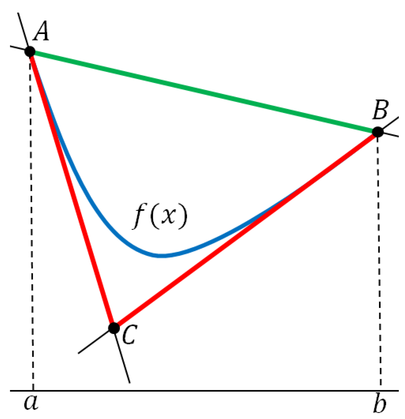
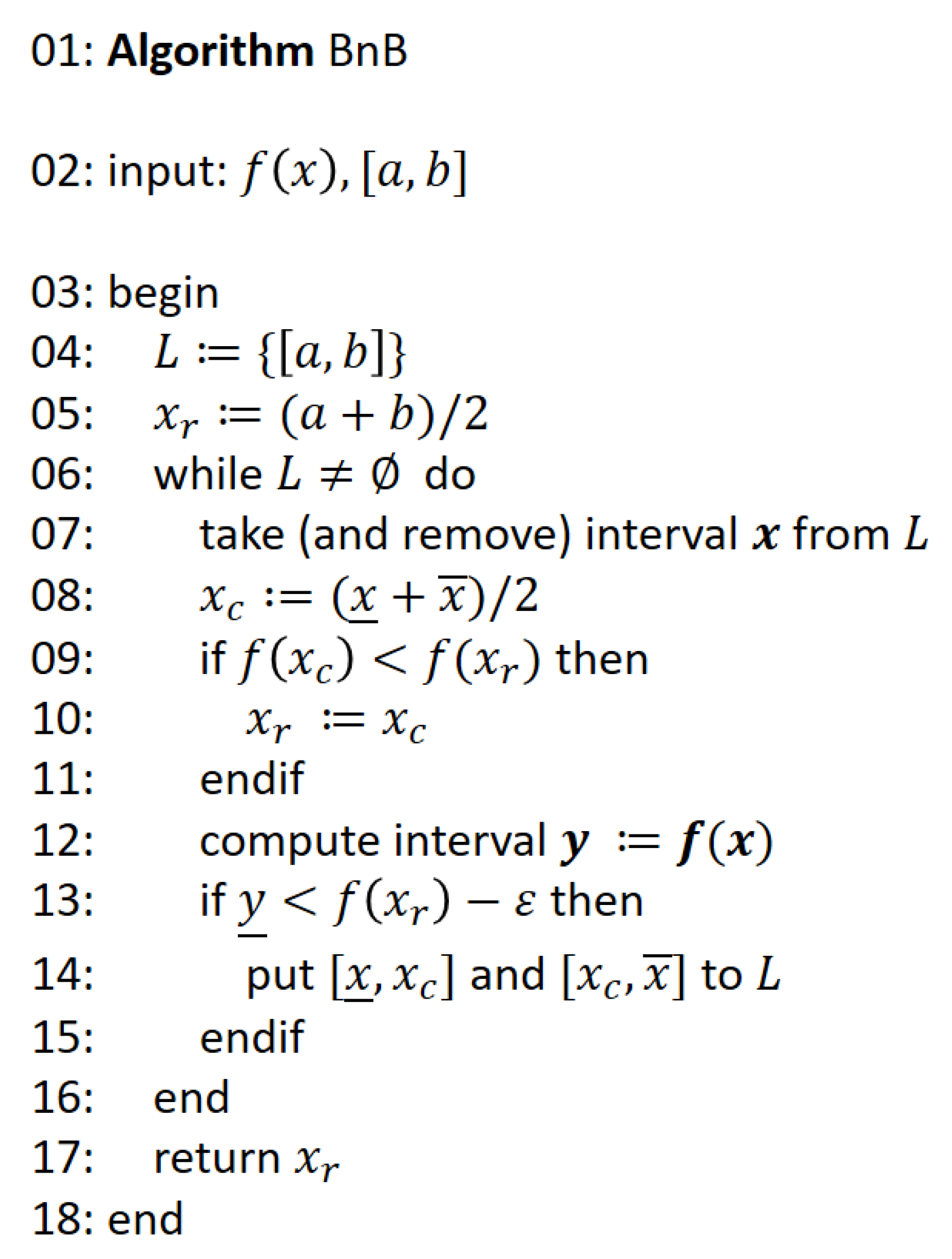
3. Application to Bounding the Function’s Range

An obvious application of the proposed techniques is the convexity/concavity test [26] that helps to eliminate the interval from the further consideration and reduce the number of steps of branch-and-bound algorithms. Consider the following problem:

$$f\left(x\right)\to min,x\in [a,b].$$

(4)

If the objective $f\left(x\right)$ is concave on $[a,b]$, then the global minimum can be easily computed as follows: $f\left(x_{*}\right)=min(f\left(a\right),f\left(b\right))$. If the concavity does not hold for the entire search region, the test can be used in branch-and-bound, interval Newton or other global minimization methods by applying it to subintervals of $[a,b]$ processed by the algorithm.

However, if the objective is convex on $[a,b]$, then any local minimum in $[a,b]$ is a global minimum and can be easily found by a local search procedure. Since any continuously differentiable function is convex or concave on a sufficiently small interval, the convexity/concavity test can tremendously reduce the number of algorithm’s steps by preventing excessive branching.

Another situation commonly encountered in practice occurs when a subexpression represents a convex/concave function while the entire function is not convex neither concave. For example, the function $0.5-cos\left(x\right)$ is convex on interval $[-\pi /2,\pi /2]$ while ${(0.5-cos\left(x\right))}^3$ is not. In such cases, the interval cannot be discarded by the convexity/concavity test. Nevertheless, the convexity and concavity can be used to compute tight upper and lower bounds for the sub-expression yielding better bounds for the entire function.

For computing upper and lower bounds, recall that a convex function graph always lies above any of its tangents. This property and the convexity definition yield the Proposition 7.

Proposition 7. 

Let $f\left(x\right)$ be a convex function on $[a,b]$. Then

$$\underline{f}\left(x\right)\le f\left(x\right)\le \overline{f}\left(x\right),for all x\in [a,b],$$

(5)

where

$$\begin{array}{cc}\hfill \underline{f}\left(x\right)& =max\left(f\left(a\right)+f^{\prime }\left(a\right)(x-a),f\left(b\right)+f^{\prime }\left(b\right)(x-b)\right),\hfill \\ \hfill \overline{f}\left(x\right)& =f\left(a\right)+(f\left(b\right)-f\left(a\right))\frac{x-a}{b-a}.\hfill \end{array}$$

(6)

Proof. 

First, prove that $\underline{f}\left(x\right)$ is an underestimator for $f\left(x\right)$. For a function $f\left(x\right)$ convex on an interval $[a,b]$ and a point $t\in [a,b]$, the following inequality holds [43]:

$$f\left(x\right)\ge f\left(t\right)+f^{\prime }\left(t\right)(x-t),\mathrm{for}\mathrm{all} x\in [a,b].$$

(7)

Substituting t with a and b in (7), we get the following system of valid inequalities:

$$\begin{array}{cc}\hfill f\left(x\right)& \ge f\left(a\right)+f^{\prime }\left(a\right)(x-a),\mathrm{for}\mathrm{all} x\in [a,b],\hfill \\ \hfill f\left(x\right)& \ge f\left(b\right)+f^{\prime }\left(b\right)(x-b),\mathrm{for}\mathrm{all} x\in [a,b].\hfill \end{array}$$

(8)

From (8), it directly follows that

$$f\left(x\right)\ge max\left(f\left(a\right)+f^{\prime }\left(a\right)(x-a),f\left(b\right)+f^{\prime }\left(b\right)(x-b)\right),\mathrm{for}\mathrm{all} x\in [a,b].$$

The right part is $\underline{f}\left(x\right)$ from (6).

Now prove that $\overline{f}\left(x\right)$ is the overestimator for $f\left(x\right)$. Taking $x_1=a$, $x_2=b$, $\lambda =\frac{b-x}{b-a}$ in the definition of a convex function (3) we obtain:

$$\begin{array}{cc}\hfill f\left(x\right)& \le \frac{b-x}{b-a}f\left(a\right)+\left(1-\frac{b-x}{b-a}\right)f\left(b\right)=\left(1-\frac{x-a}{b-a}\right)f\left(a\right)+\frac{x-a}{b-a}f\left(b\right)\hfill \\ & =f\left(a\right)+\left(f\left(b\right)-f\left(a\right)\right)\frac{x-a}{b-a}.\hfill \end{array}$$

The rightmost part is $\overline{f}\left(x\right)$ from (6). This completes the proof. □

Proposition 7 is illustrated in Figure 1. The figure shows the original function $f\left(x\right)$ (blue curve), its overestimator consisting of one green line segment and the underestimator consisting of two connected line segments $AC$ and $CB$ marked with red. The estimators are constructed by following (6).

Figure 1. The overestimator (green) and the underestimator (red) of a convex function $f\left(x\right)$ on an interval $[a,b]$.

The similar proposition holds for concave functions.

Proposition 8. 

Let $f\left(x\right)$ be a concave function over on $[a,b]$. Then

$$\underline{f}\left(x\right)\le f\left(x\right)\le \overline{f}\left(x\right),for all x\in [a,b],$$

(9)

where

$$\begin{array}{cc}\hfill \underline{f}\left(x\right)& =f\left(a\right)+(f\left(b\right)-f\left(a\right))\frac{x-a}{b-a},\hfill \\ \hfill \overline{f}\left(x\right)& =min\left(f\left(a\right)+f^{\prime }\left(a\right)(x-a),f\left(b\right)+f^{\prime }\left(b\right)(x-b)\right).\hfill \end{array}$$

(10)

Proof. 

This statement is a straightforward corollary of Proposition 7. Indeed, if $f\left(x\right)$ is concave then $-f\left(x\right)$ is convex and one can apply Formula (6) to obtain its estimators. After changing the sign and reversing the inequalities we get (10). □

Fortunately, the minimum and maximum of estimators $\underline{f}\left(x\right)$ and $\overline{f}\left(x\right)$ can be found analytically as stated by the following propositions.

Proposition 9. 

If a function f is convex on an interval $[a,b]$ then

$$\underset{x\in [a,b]}{max}f\left(x\right)=max(f\left(a\right),f\left(b\right)),$$

(11)

$$\underset{x\in [a,b]}{min}f\left(x\right)=f\left(a\right),if{f}^{\prime }\left(a\right)\ge 0,$$

(12)

$$\underset{x\in [a,b]}{min}f\left(x\right)=f\left(b\right),if{f}^{\prime }\left(b\right)\le 0,$$

(13)

$$\underset{x\in [a,b]}{min}f\left(x\right)\ge \frac{f^{\prime }\left(b\right)f\left(a\right)-f^{\prime }\left(a\right)f\left(b\right)}{f^{\prime }\left(b\right)-f^{\prime }\left(a\right)}+f^{\prime }\left(a\right)f^{\prime }\left(b\right)\frac{b-a}{f^{\prime }\left(b\right)-f^{\prime }\left(a\right)}$$

(14)

otherwise.

Proof. 

Equation (11) is obviously valid. Denote $\alpha =f^{\prime }\left(a\right)$, $\beta =f^{\prime }\left(b\right)$. Equation (12) follows from the fact the function $f\left(x\right)$ lies above its tangent $f\left(a\right)+\alpha (x-a)$, coincides with it at $x=a$ and the tangent is a monotonically nondecreasing function. In the same way, Equation (13) is proved.

For the remaining case $\alpha <0<\beta$ the minimum of the underestimator is achieved at the intersection point of lines defined by $f\left(a\right)+\alpha (x-a)$, $f\left(b\right)+\beta (x-b)$ (point C in the Figure 1). This point is the solution of the following equation:

$$f\left(a\right)+\alpha (x-a)=f\left(b\right)+\beta (x-b).$$

Simple transformations yield:

$$f\left(a\right)-f\left(b\right)+\beta b-\alpha a=x(\beta -\alpha ).$$

Since $\alpha \ne \beta$ the minimum of the underestimator is achieved at the point

$$x=\frac{f\left(a\right)-f\left(b\right)+\beta b-\alpha a}{\beta -\alpha }.$$

Substituting this value to $f\left(a\right)+\alpha (x-a)$ we obtain:

$$\underset{x\in [a,b]}{min}\underline{f}\left(x\right)=\frac{\beta f\left(a\right)-\alpha f\left(b\right)}{\beta -\alpha }+\alpha \beta \frac{b-a}{\beta -\alpha }.$$

This concludes the proof. □

Similarly, the validity of the following Proposition giving bounds for a concave function is justified.

Proposition 10. 

If a function f is concave over an interval $[a,b]$ then

$$\underset{x\in [a,b]}{min}f\left(x\right)=min(f\left(a\right),f\left(b\right)),$$

(15)

$$\underset{x\in [a,b]}{max}f\left(x\right)=f\left(a\right),if{f}^{\prime }\left(a\right)\le 0,$$

(16)

$$\underset{x\in [a,b]}{max}f\left(x\right)=f\left(b\right),if{f}^{\prime }\left(b\right)\ge 0,$$

(17)

$$\underset{x\in [a,b]}{max}f\left(x\right)\le \frac{f^{\prime }\left(b\right)f\left(a\right)-f^{\prime }\left(a\right)f\left(b\right)}{f^{\prime }\left(b\right)-f^{\prime }\left(a\right)}+f^{\prime }\left(a\right)f^{\prime }\left(b\right)\frac{b-a}{f^{\prime }\left(b\right)-f^{\prime }\left(a\right)}$$

(18)

otherwise.

Proof. 

This statement is a straightforward corollary of Proposition 9. Indeed, if $f\left(x\right)$ is concave then $-f\left(x\right)$ is convex and one can apply Formulas (11)–(14) to obtain its estimators. After changing the sign and reversing the inequalities, we get Formulas (15)–(18). □

The bounds computed with the help of the Propositions 9 and 10 are often more precise with respect to other bounds. Below we compare the ranges computed according to Propositions 9 and 10 with the results of interval analysis techniques.

4. Numerical Experiments

In this section, we experimentally evaluate the proposed approach. First, in Section 4.1 the interval bounds and bounds computed with the proposed techniques are compared for a set of functions. In Section 4.2, we study the impact of the accounting of the monotonicity and convexity properties on global optimization algorithms’ performance.

4.1. Comparison with Interval Bounds

We selected two well-known [26,28] interval analysis techniques for computing the range of a function. The first is the natural interval expansion that computes the interval bounds of a function’s range by applying interval arithmetic rules according to the function’s expression. The second approach is so-called first-order Taylor expansion:

$${\mathcal{R}}_f\left([a,b]\right)\subseteq f\left(c\right)+[a-c,b-c]·{\mathbf{f}}^{\prime }\left([a,b]\right),$$

(19)

where $c=(a+b)/2$ and ${\mathbf{f}}^{\prime }\left([a,b]\right)$ denotes the natural interval expansion for the derivative of $f\left(x\right)$. The detailed proof of (19) can be found in [26].

Example 4. 

Let $f\left(x\right)=-cos\left(x\right)+e^{-x}$ and $a=0,b=1$. The convexity of $f\left(x\right)$ can easily be established by applying evaluation rules introduced in the previous section:

• $cos\left(x\right)$ is concave on $[0,1]$,
• $-cos\left(x\right)$ is convex on $[0,1]$ (by definition),
• x is concave on $[0,1]$,
• $-x$ is convex on $[0,1]$ (by definition),
• $e^{-x}$ is convex on $[0,1]$ (by Proposition 6),
• $-cos\left(x\right)+e^{-x}$ is convex on $[0,1]$ (by Proposition 4).

Applying (9), we get the following enclosing interval for $f\left(x\right)$ on $[0,1]$:

$$f\left(\right[0,1\left]\right)\subseteq [-0.438,0],$$

with the width $0.438$. Natural interval expansion gives:

$$f\left(\right[0,1\left]\right)\subseteq [-0.632,0.46],$$

with the width $1.092$ and the first order Taylor expansion produces

$$f\left(\right[0,1\left]\right)\subseteq [-0.77,0.23]$$

with the width $1.092$. Thus, the interval computed with the proposed techniques is nearly $2.5$ times narrower than produced by the natural interval and Taylor expansions.

It is worth noting that the bounds provided by Propositions 9 and 10 can be computed for functions that are not differentiable at a set of points. It suffices that a function has its derivatives at the ends of the interval. The latter can be computed using the forward mode automatic differentiation [28], which is merely the application of differentiation rules at a point.

Table 4 compares bounds computed with the interval analysis techniques and the bounds computed by the proposed method for five convex functions. The convexity of these functions can be easily deduced by the introduced convexity evaluation rules. For an interval $[a,b]$, three bounds are presented in the respective columns:

Table 4. Comparison of natural interval expansion (Natural) Taylor expansion (Taylor) and bounds produced by the proposed techniques (Convex).

No	$\mathit{f}\left(\mathit{x}\right)$	$[\mathit{a},\mathit{b}]$	Natural	Taylor	Convex
1	$-cos\left(x\right)+e^{-x}$	$[0,1]$	$[-0.632,0.46]$	$[-0.77,0.23]$	$[-0.438,0]$
2	$e^x+e^{-x}$	$[-0.5,0.5]$	$[1.21,3.29]$	$[1.48,2.52]$	$[1.73,2.26]$
3	$0.2x^2-sin\left(x\right)$	$[0,\pi /2]$	$[-1,0.49]$	$[-1.37,0.2]$	$[-0.92,0]$
4	$2{\left(x-3\right)}^2+e^{0.5x^2}$	$[1,3]$	$[1.65,98.02]$	$[-260.66,279.44]$	$[-0.92,90.02]$
5	${\left(x-4\right)}^2+{\left(x+4\right)}^2+e^{\left|x\right|}$	$[-2,2]$	$[9,79.39]$	—	$[16.61,47.39]$

 

Natural—a bound computed by the natural interval expansion techniques,

 

Taylor—a bound computed by the 1st order Taylor expansion,

 

Convex—a bound computed according to Propositions 9 and 10.

For all functions except No. 4, the bound produced by the proposed techniques contain both intervals produced by interval techniques and significantly more tight. For function number 4, the interval computed by the Convex method is narrower than the natural interval expansion but does not enclose it. However, as neither of these intervals contains each other, they can be intersected to obtain a better enclosing interval $[1.65,90.02]$. The 5th function is non-differentiable in $x=0$. Thus the symbolic differentiation does not give a meaningful result, and the Taylor expansion cannot be applied in this case. For that reason, the respective cell is marked with “−”.

4.2. Impact on the Performance of Global Search

In Section 4.1, we observed that accounting convexity can significantly improve the interval bounds. As expected, the application of these bounds entails reducing the number of steps of the global search algorithm.

We implemented a standard branch-and-bound algorithm that uses the lower-bound test to discard subintervals from the further search. The description of this algorithm can be found elsewhere [26,41]. For completeness, we outline it here (Figure 2).

Figure 2. The standard branch-and-bound algorithm.

The algorithm operates over a list L of intervals, initialized with the feasible set $[a,b]$ (line 04). The record point (incumbent solution) is initialized with the center of the interval $[a,b]$ (line 05). The main loop (lines 06—16) iterates until the list L is not empty. At each iteration one of the intervals from this set is taken (line 07) and examined. First, the value in the middle of this interval is computed, and if necessary, the record is updated (lines 08–11). The interval extension $\mathbf{y}=\mathbf{f}\left(\mathbf{x}\right)$ is computed at the line 12. The interval lying above $f\left(x_r\right)-\epsilon$ is discarded from the further search. Otherwise, it is partitioned into two smaller intervals. The obtained intervals are added to the list L (line 14).

We consider three variants of computing the interval extension:

• Natural—the natural interval expansion techniques,
• Taylor—the 1-st order Taylor expansion,
• Convex—the range is computed according to Propositions 3, 9 and 10.

The described methods can be applied in combination, when the intervals computed by several methods are intersected to obtain the resulting range. We considered four different combinations of the range bounding techniques to compute the enclosing interval of the objective function:

• Natural—pure natural interval expansion;
• Natural + Convex—the natural interval expansion combined with the proposed techniques;
• Natural + Taylor—the natural interval expansion combined with the first-order Taylor expansion;
• Natural + Taylor + Convex—the natural interval expansion combined with the first-order Taylor expansion and the proposed techniques.

The convexity and the monotonicity are detected by analyzing the ranges of the first/second derivatives in differentiable cases or by using the introduced evaluation rules for the non-differentiable expressions.

Table 5 lists the set of test problems used in the experiments. For each problem, the objective function ($f\left(x\right)$), the interval ($[a,b]$), and the global optimum value ($f\left(x_{*}\right)$) are presented. The first ten problems are taken from [29]. The objective functions in these problems have both first and second derivatives.

Table 5. Test problems.

No	$\mathit{f}\left(\mathit{x}\right)$	$[\mathit{a},\mathit{b}]$	$\mathit{f}\left({\mathit{x}}_{*}\right)$
1	${\left(x-1\right)}^2+{\left(-x^2+x\right)}^2$	$[-10,10]$	0
2	$24x^4-142x^3+303x^2-276x+3$	$[0,3]$	1
3	$x^4-12x^3+47x^2-60x-20e^{-x}$	$[-1,7]$	$-32.781261$
4	$x^4-10x^3+35x^2-50x+24$	$[-10,20]$	$-1$
5	$-1.5{sin}^2\left(x\right)+sin\left(x\right)cos\left(x\right)+1.2$	$[0.2,7]$	$-0.451388$
6	$-x+sin\left(3x\right)+1$	$[0.2,7]$	$-5.815675$
7	$x+sin\left(5x\right)$	$[0.2,7]$	$-0.07759$
8	$-sin\left(5x\right)+cos\left(x\right)+1$	$[0.2,7]$	$-0.952897$
9	$2cos\left(x\right)+cos\left(2x\right)+5$	$[0.2,7]$	$3.5$
10	$2e^{-x}sin\left(x\right)$	$[0.2,7]$	$-0.027864$
11	$\left|x\right|+\left|x-4\right|+\left|x+4\right|$	$[-8,8]$	8
12	${\left(x-4\right)}^2+{\left(x+4\right)}^2+e^{\left|x\right|}$	$[-4,8]$	33
13	$\left|(x-1)/4\right|+\left|sin\left(\pi (1+(x-1)/4)\right)\right|+1$	$[-10,10]$	1
14	$\left(10\left|sin\left(x+1\right)\right|+1\right)\left|x-1\right|+1$	$[-10,10]$	1

To demonstrate the applicability of the proposed automatic convexity deduction techniques, we also have added four nondifferentiable problems. Test cases 11 and 12 were proposed by us, and 13 and 14 were taken from [33].

The results of numerical experiments are summarized in Table 6. The cells contain the number of steps performed by the branch-and-bound method. Columns correspond to different ways for computing the range of the objective functions, and rows correspond to test problems. The Taylor expansion cannot be applied to nondifferentiable problems 11–14, and the respective cells are blank.

Table 6. Testing results.

No	Natural	Natural + Convex	Natural + Taylor	Natural + Taylor + Convex
1	35	15	29	15
2	135,043	199	267	81
3	98,995	107	269	79
4	72,953	151	311	91
5	443	39	83	39
6	187	19	47	19
7	183	39	69	39
8	189	49	91	49
9	857	31	75	31
10	51	19	27	19
11	55	5	—	—
12	579	23	—	—
13	35	27	—	—
14	125	125	—	—

Experimental results demonstrate that the proposed techniques tremendously improve the standard branch-and-bound algorithm’s performance that uses the natural interval expansion for the majority of the test problems. The combination of the natural interval expansion and the proposed method always outperform the combination of the natural and the first-order Taylor interval expansion. The comparison of the last two columns of Table 6 indicates that the Taylor expansion version of branch-and-bound can be further improved when combined with the proposed techniques. However, for problems 1 and 5–10, the proposed method does not benefit from the Taylor expansion.

5. Discussion

The standard way to ensure the convexity is to bound the range of the function’s second derivative. However, this approach is only applicable to smooth functions. We defined a set of rules that can efficiently handle nonsmooth functions. The algebraic representation for the function, however, should be available.

It is worth noting that the proposed approach can be efficiently coded in modern programming languages supporting the operator’s overloading techniques. To run the experiments presented in Table 4 and Table 6 we have implemented our approach in Python. The elementary functions and operators were overloaded to support a particular data type that carries monotonicity and convexity information and the range of the function. The overloaded methods work according to the rules described in Section 2 and interval arithmetic.

As we have shown above, evaluating convexity can improve interval bounds on the function’s range and accelerate the global optimization algorithms. Moreover, the over- and underestimators defined by the Propositions 7 and 8 enable efficient reduction techniques. The reduction techniques are widely used to accelerate the search for a global minimum of a function or a root of an equation.

We believe that the proposed approach has great potential as it can be extended to various generalized notions of convexity, e.g., quasiconvexity [46]. Quasiconvex functions possess the unimodality property, and thus recognizing the quasiconvexity (quasiconcavity) can tremendously enhance global optimization algorithms.

References

- Johnson, D.E. Introduction to Filter Theory; Prentice Hall: Englewood Cliffs, NJ, USA, 1976. [Google Scholar]
- Zilinskas, A. Optimization of one-dimensional multimodal functions. J. R. Stat. Soc. Ser. C Appl. Stat. 1978, 27, 367–375. [Google Scholar]
- Kvasov, D.; Menniti, D.; Pinnarelli, A.; Sergeyev, Y.D.; Sorrentino, N. Tuning fuzzy power-system stabilizers in multi-machine systems by global optimization algorithms based on efficient domain partitions. Electr. Power Syst. Res. 2008, 78, 1217–1229. [Google Scholar] [CrossRef]
- Bedrosian, D.; Vlach, J. Time-domain analysis of networks with internally controlled switches. IEEE Trans. Circuits Syst. I Fundam. Theory Appl. 1992, 39, 199–212. [Google Scholar] [CrossRef]
- Femia, N.; Tucci, V. On the modeling of PWM converters for large signal analysis in discontinuous conduction mode. IEEE Trans. Power Electron. 1994, 9, 487–496. [Google Scholar] [CrossRef]
- Lassere, J.B. Connecting optimization with spectral analysis of tri-diagonal matrices. Math. Program. 2020. [Google Scholar] [CrossRef]
- Strongin, R.G.; Sergeyev, Y.D. Global Optimization with Non-Convex Constraints: Sequential and Parallel Algorithms; Springer Science & Business Media: Berlin/Heidelberg, Germany, 2013; Volume 45. [Google Scholar]
- Lera, D.; Sergeyev, Y.D. GOSH: Derivative-free global optimization using multi-dimensional space-filling curves. J. Glob. Optim. 2018, 71, 193–211. [Google Scholar] [CrossRef]
- Lera, D.; Posypkin, M.; Sergeyev, Y.D. Space-filling curves for numerical approximation and visualization of solutions to systems of nonlinear inequalities with applications in robotics. Appl. Math. Comput. 2021, 390, 125660. [Google Scholar] [CrossRef]
- Jensen, P.A.; Bard, J.F.; Jensen, P. Operations Research Models and Methods; John Wiley & Sons: Hoboken, NJ, USA, 2003. [Google Scholar]
- Pintér, J. Extended univariate algorithms for n-dimensional global optimization. Computing 1986, 36, 91–103. [Google Scholar] [CrossRef]
- Sergeyev, Y.D.; Kvasov, D.E. Deterministic Global Optimization: An Introduction to the Diagonal Approach; Springer: Berlin/Heidelberg, Germany, 2017. [Google Scholar]
- Evtushenko, Y.G. Numerical methods for finding global extrema (case of a non-uniform mesh). USSR Comput. Math. Math. Phys. 1971, 11, 38–54. [Google Scholar] [CrossRef]
- Pijavskij, S. An algorithm for finding the global extremum of function. Optim. Decis. 1967, 2, 13–24. [Google Scholar]
- Shubert, B.O. A sequential method seeking the global maximum of a function. SIAM J. Numer. Anal. 1972, 9, 379–388. [Google Scholar] [CrossRef]
- Timonov, L. Algorithm for search of a global extremum. Eng. Cybern. 1977, 15, 38–44. [Google Scholar]
- Jones, D.R.; Perttunen, C.D.; Stuckman, B.E. Lipschitzian optimization without the Lipschitz constant. J. Optim. Theory Appl. 1993, 79, 157–181. [Google Scholar] [CrossRef]
- Kvasov, D.E.; Sergeyev, Y.D. A univariate global search working with a set of Lipschitz constants for the first derivative. Optim. Lett. 2009, 3, 303–318. [Google Scholar] [CrossRef]
- Lera, D.; Sergeyev, Y.D. Acceleration of univariate global optimization algorithms working with Lipschitz functions and Lipschitz first derivatives. SIAM J. Optim. 2013, 23, 508–529. [Google Scholar] [CrossRef]
- Gergel, V.P. A global optimization algorithm for multivariate functions with Lipschitzian first derivatives. J. Glob. Optim. 1997, 10, 257–281. [Google Scholar] [CrossRef]
- Sergeyev, Y.D. Global one-dimensional optimization using smooth auxiliary functions. Math. Program. 1998, 81, 127–146. [Google Scholar] [CrossRef]
- Sergeyev, Y.D.; Nasso, M.C.; Mukhametzhanov, M.S.; Kvasov, D.E. Novel local tuning techniques for speeding up one-dimensional algorithms in expensive global optimization using Lipschitz derivatives. J. Comput. Appl. Math. 2020, 383, 113134. [Google Scholar] [CrossRef]
- Hansen, P.; Jaumard, B.; Lu, S.H. Global optimization of univariate Lipschitz functions: I. Survey and properties. Math. Program. 1992, 55, 251–272. [Google Scholar] [CrossRef]
- Hansen, P.; Jaumard, B.; Lu, S.H. Global optimization of univariate Lipschitz functions: II. New algorithms and computational comparison. Math. Program. 1992, 55, 273–292. [Google Scholar] [CrossRef]
- Pintér, J.D. Global Optimization in Action: Continuous and Lipschitz Optimization: Algorithms, Implementations and Applications; Springer Science & Business Media: Berlin/Heidelberg, Germany, 2013; Volume 6. [Google Scholar]
- Hansen, E.; Walster, G.W. Global Optimization Using Interval Analysis: Revised and Expanded; CRC Press: Boca Raton, FL, USA, 2003; Volume 264. [Google Scholar]
- Moore, R.E.; Kearfott, R.B.; Cloud, M.J. Introduction to Interval Analysis; SIAM: Philadelphia, PA, USA, 2009. [Google Scholar]
- Kearfott, R.B. Rigorous Global Search: Continuous Problems; Springer Science & Business Media: Berlin/Heidelberg, Germany, 2013; Volume 13. [Google Scholar]
- Casado, L.G.; MartÍnez, J.A.; GarcÍa, I.; Sergeyev, Y.D. New interval analysis support functions using gradient information in a global minimization algorithm. J. Glob. Optim. 2003, 25, 345–362. [Google Scholar] [CrossRef]
- Fasano, G.; Pintér, J.D. Efficient piecewise linearization for a class of non-convex optimization problems: Comparative cesults and extensions. In Springer Proceedings in Mathematics & Statistics; Pintér, J., Terlaky, T., Eds.; Springer: Berlin/Heidelberg, Germany, 2019; Volume 279, pp. 39–56. [Google Scholar]
- Posypkin, M.; Usov, A.; Khamisov, O. Piecewise linear bounding functions in univariate global optimization. Soft Comput. 2020, 24, 17631–17647. [Google Scholar] [CrossRef]
- Floudas, C.; Gounaris, C. Tight convex underestimators for C2-continuous functions: I. Univariate functions. J. Glob. Optim 2008, 42, 51–67. [Google Scholar]
- Ratz, D. A nonsmooth global optimization technique using slopes: The one-dimensional case. J. Glob. Optim. 1999, 14, 365–393. [Google Scholar] [CrossRef]
- Tuy, H.; Hoang, T.; Hoang, T.; Mathématicien, V.N.; Hoang, T.; Mathematician, V. Convex Analysis and Global Optimization; Springer: Berlin/Heidelberg, Germany, 1998. [Google Scholar]
- Strekalovsky, A.S. On local search in dc optimization problems. Appl. Math. Comput. 2015, 255, 73–83. [Google Scholar]
- Arıkan, O.; Burachik, R.; Kaya, C. Steklov regularization and trajectory methods for univariate global optimization. J. Glob. Optim. 2020, 76, 91–120. [Google Scholar] [CrossRef]
- Ahmadi, A.; Hall, G. On the complexity of detecting convexity over a box. Math. Program. 2020, 182, 429–443. [Google Scholar] [CrossRef]
- Fourer, R.; Maheshwari, C.; Neumaier, A.; Orban, D.; Schichl, H. Convexity and concavity detection in computational graphs: Tree walks for convexity assessment. Informs J. Comput. 2010, 22, 26–43. [Google Scholar] [CrossRef]
- Grant, M.; Boyd, S. CVX: MATLAB Software for Disciplined Convex Programming. Version 1.21. 2010. Available online: http://cvxr.com/cvx (accessed on 9 January 2020).
- Grant, M.C.; Boyd, S.P. Graph implementations for nonsmooth convex programs. In Recent Advances in Learning and Control; Springer: Berlin/Heidelberg, Germany, 2008; pp. 95–110. [Google Scholar]
- Ratschek, H.; Rokne, J. New Computer Methods for Global Optimization; Horwood: Chichester, UK, 1988. [Google Scholar]
- Nataraj, P.S.; Arounassalame, M. A new subdivision algorithm for the Bernstein polynomial approach to global optimization. Int. J. Autom. Comput. 2007, 4, 342–352. [Google Scholar] [CrossRef]
- Boyd, S.; Vandenberghe, L. Convex Optimization; Cambridge University Press: Cambridge, UK, 2004. [Google Scholar]
- Nesterov, Y. Introductory Lectures on Convex Optimization: A Basic Course; Springer Science & Business Media: Berlin/Heidelberg, Germany, 2013; Volume 87. [Google Scholar]
- Niculescu, C.; Persson, L.-E. Convex Functions and their Applications. A Contemporary Approach; Springer International Publishing: Berlin/Heidelberg, Germany, 2018. [Google Scholar]
- Hadjisavvas, N.; Komlósi, S.; Schaible, S.S. Handbook of Generalized Convexity and Generalized Monotonicity; Springer Science & Business Media: Berlin/Heidelberg, Germany, 2006; Volume 76. [Google Scholar]
Publisher’s Note: MDPI stays neutral with regard to jurisdictional claims in published maps and institutional affiliations. |
© 2021 by the authors. Licensee MDPI, Basel, Switzerland. This article is an open access article distributed under the terms and conditions of the Creative Commons Attribution (CC BY) license (http://creativecommons.org/licenses/by/4.0/).