1. Introduction
One of the fundamental problems studied in Control Engineering concerns robustness, which characterizes the sensitivity of the closed loop system to the variation of plant parameters. One of the most used performance measures is the
norm. Starting from the approach of synthesizing a
controller by solving two Algebraic Riccati Equations (AREs) as in [
1], a more numerically stable solution can be obtained using Popov triplets [
2]. Alternatively, due to the limitations of this approach represented by the impossibility of solving singular problems, the AREs were replaced with Algebraic Riccati Inequalities (ARIs) and were solved using Linear Matrix Inequalities (LMIs) [
3]. The last two approaches have been recently implemented in open-source manners in [
4,
5]. However, the classical
control problem manages to ensure nominal stability and nominal performance only. In order to consider dynamic and parametric uncertainties, the plant is formulated as an upper linear fractional transform with such an uncertainty block and the
-synthesis can be used for computing a robust controller based on the classical
D–
K iterations [
6]. The major concern about these methods consists of the fact that the controller is usually of high order. However, imposing a fixed structure leads to a non-convex problem which cannot be approximated as in the case of
-synthesis. The solutions, initially proposed for
problem [
7], and then for
-synthesis [
8] as well, are based on nonsmooth optimization techniques. A CACSD toolbox that manages to offer an end-to-end solution for designing a robust controller starting from a given plant is presented in [
9].
The most well-known controller structure, which is highly used in industry, is the proportional-integral-derivative (PID) regulator. Its form is generally given as an example for fixed-structure controllers and nonsmooth optimization methods were designed around it [
10]. An extension with two extra degrees of freedom is represented by fractional-order PID (FO-PID), which improves the robustness of the closed loop system. As tuning methods, the well-known methods used for designing integer-order controllers were extended for fractional-order controllers as well. As such, two generalized versions of Kessler’s magnitude methods were presented in [
11,
12], while a fractional-order internal model controller with event-based implementation was developed in [
13]. A fractional-order integrator was used as a model for the servo problem in [
14], while the same structure was used as a speed controller for a DC motor in [
15]. In [
16]
crone control methodologies were presented, along with LMI formulation for the
fractional-order control problem. An artificial bee colony optimization for a MIMO FO-PID controller design by solving the mixed-sensitivity
-synthesis control problem is presented in [
17].
The twin rotor aerodynamic system (TRAS) is a well-known benchmark system used to illustrate the control methods designed in literature. A two degrees of freedom (2-DOF) discrete-time
-synthesis controller of order 24 was presented in [
18]. A decentralized fixed-structure PID controller designed using
is presented in [
19], along with a comparison between the full-order
controller. After the linearization and decoupling steps, 2-DOF continuous and discrete-time controllers were designed using
in [
20]. A hybrid architecture using both
and Iterative Learning Control is described in [
21]. A linear quadratic regulator (LQR) for MIMO TRAS problem was designed using particle swarm optimization in [
22], while a frequency-based PID controller was combined with a lead compensator designed using root locus in [
23]. An approach that further details the controller implementation with quantization aspects taken into consideration for the same family of processes is presented in [
24].
In this paper, we present a design procedure that manages to optimize the controller parameters instead of tuning them. As such, we present a method for finding the parameters of a MIMO fractional-order PID (FO-PID) robust controller by solving a fixed-structure mixed-sensitivity loop shaping -synthesis control problem. Although the resulting control problem is nonconvex in terms of the controller’s free parameters, the nonsmooth optimization techniques implemented in MATLAB’s Robust Control Toolbox can be used. However, the realp object used for these free parameters does not support exponential operations necessary in the approximation of a fractional-order element. Therefore, we present in this paper an algorithm to construct the approximation function of a fractional-order element using integer-order elements and supported arithmetic operations applied on a free parameter isomorphic to the desired fractional order. As such, we successfully manage to formulate the problem of optimizing the parameters of a MIMO FO-PID such that the available techniques can be used. Moreover, we illustrate our design method on the twin rotor aerodynamic system stand, having both MATLAB simulations and physical experiments.
The remainder of this paper is organized as follows:
Section 2 summarizes the main mathematical background in terms of available results in both Robust and Fractional-Order Control, along with the description of the proposed method in terms of the algorithm for approximation of the fractional order element and of the optimization problem;
Section 3 starts with the presentation of the simplified nonlinear mathematical model of the TRAS system, the linearized mathematical model around an equilibrium point, and a list of parameters with their numerical values and tolerances which manages to encompass the nonlinearities; in
Section 4, the numerical results are presented, starting from the augmentation step, followed by the proposed structure of the controller and the obtain results in MATLAB and on the experimental stand;
Section 5 presents the discussions of the obtained results and a comparison with another method for solving the optimization problem, while in
Section 6 there are some conclusions and possible research directions.
2. Proposed Method
In this section, the mathematical background for the proposed controller design method in terms of Robust Control Framework in
Section 2.1 and Fractional-Order Control Framework in
Section 2.2 is firstly presented, while in
Section 2.3 the method for optimizing the controller parameters using a different approach as against the procedure presented in [
17] is described.
2.1. Robust Control
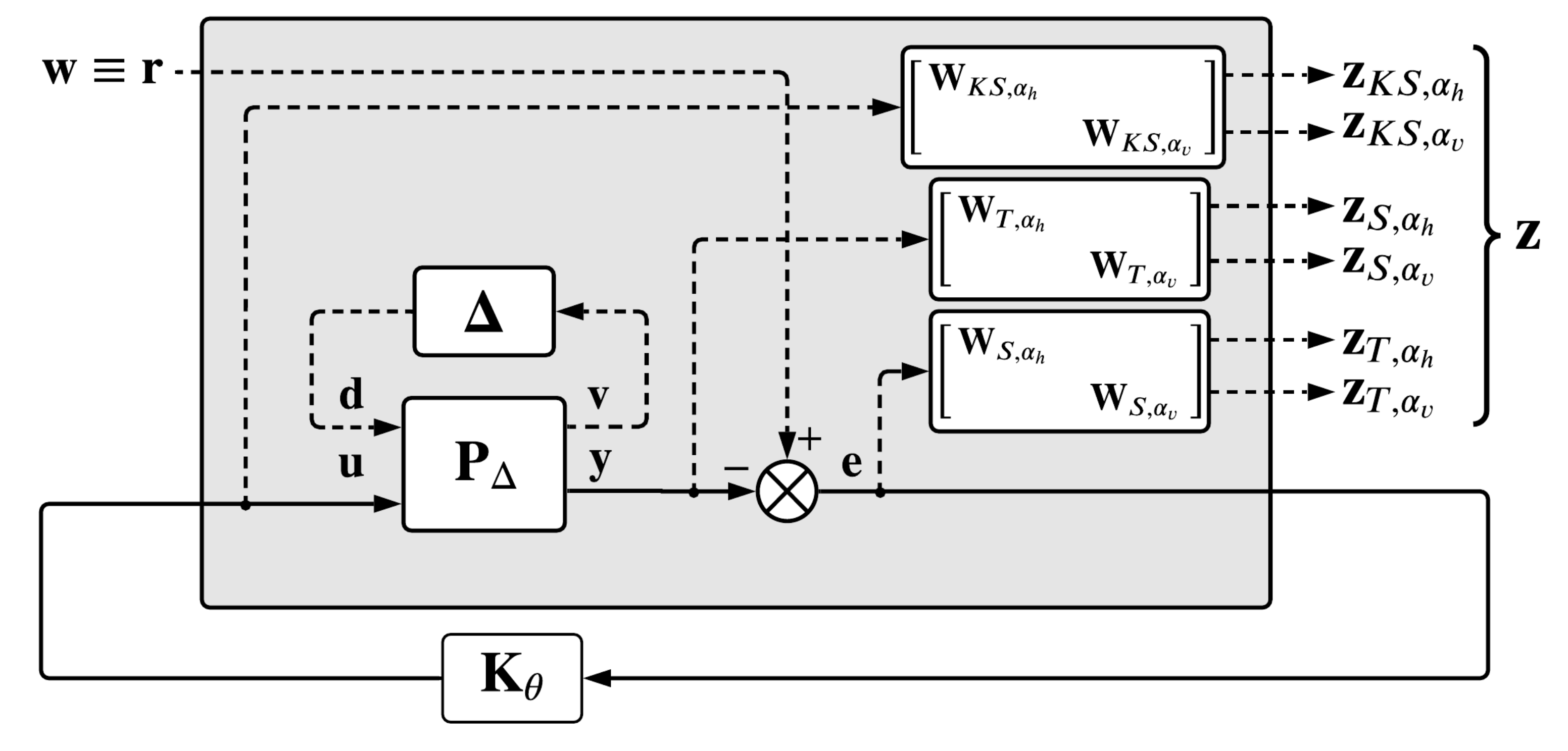
The generalized Robust Control Framework [
25] has, besides the control input vector
, two extra inputs: the exogenous input vector
and disturbance input vector
. Additionally, besides the output vector
, the generalized plant contains two extra outputs: the performance vector
and the disturbance output
. The input and output disturbance vectors encompass both parametric and unstructured uncertainties, which are generally modeled by the following set:
where
denotes the identity matrix of order
n.
The uncertainty block
is interconnected with the generalized plant
via an upper linear fractional transformation (ULFT), while the controller
K is interconnected via a lower linear fractional transformation (LLFT) with
, as noticed in
Figure 1.
The state-space representation of the generalized plant
is:
For robustness analysis, the singular value notion used for
synthesis was extended to the
structural singular value, defined for the LLFT interconnection between the plant
and the controller
K according to the uncertainty block
as:
Given that the problem of explicitly computing such structural singular values is NP-hard, an approximation must be used. The classical
control problem can be extended to the following optimization problem:
which can be considered solved if there is a controller
K such that
, according to main loop theorem. As such, an upper bound is necessary for
[
6]:
where the set
is defined according to the uncertainty block
as follows [
6]:
Summarizing, robust stability and robust performance are achieved through a controller
K obtained as a solution of the optimization problem (
4) which manages to obtain an objective value lower than 1. But this NP-hard problem can be approximated by the following quasi-convex problem:
As already known, the last optimization problem can be solved using the so-called
D–
K iteration [
9,
17]. This iterative procedure starts with a fixed
D (usually considered the unitary system) and alternatively computes the controller
K, by solving the
control problem with fixed
D, and the
D-scale factor, by solving the Parrot problem, as defined in [
6], for each point from a frequency set
followed an approximation of the obtained solutions with a minimum phase system. Therefore, after setting the initial
D-scale step as
, the following steps are successively applied:
- 1:
The
D-scale step is fixed and the controller can be computed as:
- 2:
The controller
K is fixed and the following set of convex problems must be solved:
for a given frequency range
and, then, a stable minimum phase transfer matrix
is fitted.
Steps 1 and 2 are executed in a loop sequence until the difference between two consecutive norms is less than a prescribed tolerance, the maximum number of iterations is reached, or the improvement after a prescribed number of steps is under an imposed tolerance.
2.2. Fractional-Order Control
The domain of Fractional-Order Control has recently gained more attention due to their robustness. The fractional integral operator used in Control Engineering is [
26]:
where
is the Euler Gamma function. In a similar manner with the integer order integral operator, the fractional order integral operator
has the following Laplace transform:
As previously stated, the fractional-order calculus can be used to extend the classical 3-DOF proportional-integral-derivative (PID) controller to a fractional-order PID (FO-PID) having two extra DOF
– the order of the integral operator and the order of the derivative operator, respectively. As such, based on the error signal
, the command signal
has the following expression:
where
would be
and
would be
according to the generalized framework from
Figure 1, while the differences between the transfer functions of these two controllers are:
The main drawback of the FO-PID revolves around the implementation of the fractional order elements. One possible solution is the Oustaloup recursive approximation (ORA) introduced in
crone toolbox [
16]. The approximation of a fractional-order element
with an integer-order one is detailed for
, but it can be easily extended for
. The ORA representation receives as inputs three parameters: the order
N of the LTI system which approximates the fractional-order element, along with the lower bound
and the upper bound
of the frequency range where the approximation is valid. The LTI approximation is:
where the poles and zeros frequencies can be computed using two coefficients:
followed by the recursive relations:
The MATLAB object
realp used for fixed-structure robust synthesis does not allow the use of operations other than classical arithmetic operations. Therefore, the recursive fractional-order approximation (
14) cannot be used as is in order to compute the fractional-order of the integrative and derivative effects. In
Section 2.3 we will give a possible implementation in order to use the
realp object for optimizing the controller parameters.
2.3. Controller Design Procedure
Although the controller which results by solving the quasi-convex problem (
7) manages to fulfill the robust stability and robust performance, the major drawback consists in the fact that the controller is of high-order and cannot be easily implemented. As such, the problem should be constrained to use a specific controller structure. After imposing a fixed-structure family
, the problem (
7) can be written as:
The above problem is non-convex in terms of the free tuning parameters of the controller
. However, the problem (
17) can also be solved using the
D–
K iteration approach, where the
K step from (
8) is replaced with the following
step:
In the MATLAB environment there exists the
realp object which can be used to construct a desired family of controllers
and then the closed loop system contains both uncertainties and free tunable parameters alike. Using nonsmooth optimization techniques presented in [
8] and implemented in [
25], the fixed-structure
-synthesis control problem can be solved. For the purpose of this paper, we consider the fixed structure controller family:
where each controller
has the form:
having the free parameters:
However, the tunable parameters
and
cannot be used as
realp objects, due to exponential operations not supported. As a solution, ORA is used with the tunable parameter being
from (
15). The transfer function (
14) can be implemented using
as in Algorithm 1.
| Algorithm 1: Construct Fractional-Order Element |
![Mathematics 09 02504 i001]() |
Therefore, the tunable parameters for each controller
are:
with the special mention that the parameters
and
must be in the domain
. If a desired fractional order
is out of the admissible domain, extra integrator/derivative terms can be added. Therefore, the fixed-structure
-synthesis control problem can be solved in MATLAB from the desired family
from (
19).
Additionally, the control problem will be posed in a mixed-sensitivity loop shaping -synthesis formulation. The main reason for this choice consists in the fact that the mixed-sensitivity loop shaping allows an adequate trade-off between robustness and performance. In the optimization process, the following functions will be used for the loop shaping procedure: the sensitivity function S, the complementary sensitivity function T, and the control effort . For each performance function, a set of performance outputs are considered, while the performance inputs are considered as the references.
On one hand, large magnitude in the open loop system implies good reference tracking, disturbance rejection, and unstable plant stabilization. On the other hand, small magnitude of the open loop system ensures robust stability and mitigation of measurement noise. Moreover, a small magnitude of the control effort is necessary to relieve actuator stress. Although all these magnitude requirements seem to lead to an impossible combination, the target frequency ranges for each component are disjunctive. Through the loop shaping mechanism, the engineer is supposed to find three weighting functions, one for each of the previously-mentioned closed loop performances and the frequency performance imposed by the weighting functions is strongly correlated to the corresponding time performance.
For the sensitivity function, the frequency performance indicators of the weighting function are the minimum bandwidth frequency
, which is inversely proportional with the rise time, the maximum magnitude
at low frequencies, which imposes the maximum steady-state error, the peak magnitude
, which limits the overshoot of the system, along with the imposed slope
of the sensitivity function at low and medium frequencies [
9]:
Similarly, the complementary sensitivity’s weighting function can be constructed using the peak amplitude
, the maximum magnitude at high frequencies
, the minimum bandwidth
and the roll-off
:
The control effort is generally weighted by imposing the magnitude at low and high frequencies, along with an intermediate point of interest. However, the main goal is to maintain the control effort in the range given by the saturation of the physical actuator. For MIMO systems, the weighting matrices are diagonal concatenations of the weighting functions described above. Now the optimization problem that needs to be solved for the proposed method is the mixed-sensitivity fixed-structure loop shaping
-synthesis:
3. Mathematical Model of a TRAS
The TRAS model is of sixth order with four inputs and two outputs. The state variables considered are the rotational speed of the tail rotor (
), the rotational speed of the main rotor (
), the azimuth velocity of TRAS beam (
), the pitch velocity of TRAS beam (
), the azimuth position (
), and the pitch position (
), the state vector being:
There are two control inputs,
and
, representing the normalized horizontal and vertical DC-motor PWM duty cycles, while the considered outputs will be the azimuth and pitch positions of the TRAS beam:
The TRAS model is strongly nonlinear even under some simplifying assumptions, as stated in [
27]. One simplification is regarding to the characteristics of the two rotors: their models are supposed to be of first order containing the moment of inertia and the velocity gain for each rotor. Moreover, the angular velocities of the TRAS beam is influenced by the aerodynamic force of each rotor, which is nonlinear in terms of its rotational speed, by the aerodynamic damping torque and by the cross momentum. Moreover, the azimuth velocity is strongly influenced by the pitch angle position, while the pitch velocity is influenced by the pitch angle as well by the return torque. The nonlinear model after some simplifying assumptions can be written as:
All parameters of both linearized an nonlinear systems are described in
Table 1. The first step of the linearization process is to find approximations for the functions
and
such that the two systems from inputs to rotational speeds of the rotors are of first order. In order to obtain this scenario, these functions are estimated as
and
, while the nonlinerity is treated using the sector bound technique, being included in the tolerance of each velocity gain. Moreover, the forces developed by each axis are also nonlinear in terms of rotational speeds of the rotors and can be approximated
and
, where the trust coefficients encompass the nonlinearities in their tolerances. All sector bound nonlinearites described above are depicted in
Figure 2.
After this first step, the nonlinear model can be now linearized around an equilibrium point. The forced equilibrium point has been chosen such that the outputs are
= 0 [rad], i.e., plant stabilization problem. In order to obtain this point, the state vector has the rest of the components
[rad/s],
[rad/s],
[rad/s],
[rad/s], while the input vector has the components
and
. According to [
27], the moment of inertia with respect to the horizontal axis is constant, while around the vertical axis the moment of inertia is nonlinear, having the expression
. In practice, we will consider this parameter uncertain, having the nominal value
, along with a tolerance of
. The uncertainties from the thrust coefficients of the tail and the main rotors are necessary in order to compensate the nonlinearity of the aerodynamic forces from these rotors. The friction coefficients in the axes and the cross moments coefficients also present uncertainties in order to compensate the nonlinearities presented in the angular velocity parts and the interconnections between the two rotations. The return torque coefficient is a nonlinear function in terms of pitch position and velocity, which can be approximated by an uncertain parameter having the nominal value
, and a tolerance of
. As such, the linearized state-space model can now be written as:
The singular values of the twin rotor aerodynamic system plant having the parameters presented in
Table 1, before augmentation, are presented in
Figure 3.
4. Numerical Results
The controller design procedure proposed in this paper will be applied on a twin rotor aerodynamic system (TRAS). The physical stand from INTECO [
27] is presented in
Figure 4. The numerical values of the parameters described in
Section 3 are presented in
Table 1, along with their nominal values and tolerances.
In order to illustrate the power of the proposed method, a comparison between the numerical simulations for the linearized system using MATLAB and the experimental results on the physical stand has been performed. For the numerical results, the block diagram is presented in
Figure 5, where the reference signals
are considered the inputs of the linearized system, while the performance output vector is:
For the numerical simulation part, the plant augmentation has been done with the following weighting functions parameters:
[rad/s],
[rad/s],
,
,
(the reference is considered to be a unity step signal),
[rad/s],
[rad/s],
,
,
, while the
component of the control effort weighting functions is 1, being the maximum value of the command signal, and the maximum value at high-frequency is of magnitude 5. The weighting functions result as follows:
As noted in
Figure 3, the frequency range is between
[rad/s] and
[rad/s], which will be also used for ORA, along with the order of approximation
. Using the augmented plant presented in
Figure 5, the fixed-structure mixed-sensitivity loop shaping
-synthesis problem (
25) is solved using the
musyn command from MATLAB with the following specifications: the maximum number of
D–
K iterations is 10, the threshold for the upper bound of the
is 1, and the maximum number of iterations for asserting the lack of progress is 4.
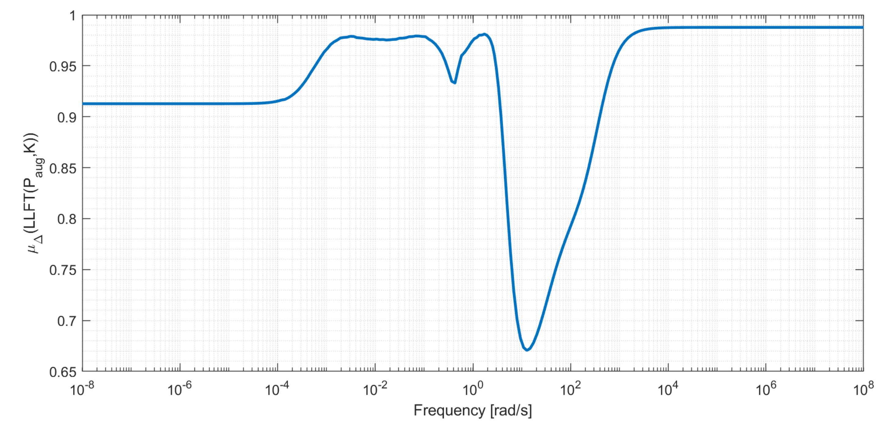
The fixed-structured
-synthesis control problem was solved using three
D–
K iterations, having the upper bound of the structured singular value
, which means that the resulting FO-PID controller manages to fulfill both robust stability and robust performance. The resulting FO-PID controller is:
where the low-pass component needs to be added in order to implement the derivative element of order greater than 1 having one extra degree of freedom for each such element. The results obtained after each step are summarized in
Table 2, where after x steps the controller design problem has been successfully solved. The upper bound of the structural singular value is presented in
Figure 6.
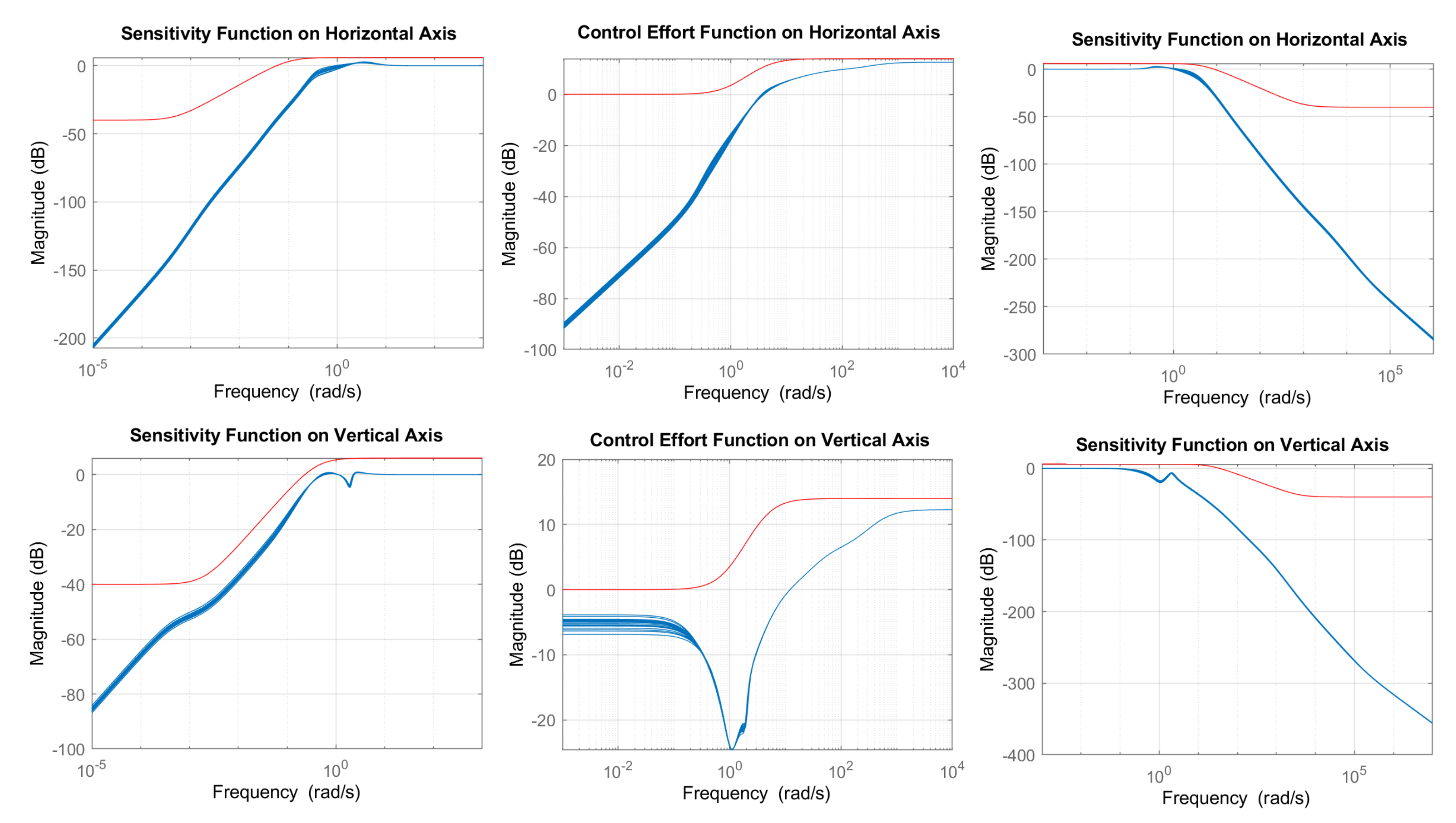
In order to illustrate the frequency-domain performance, the sensitivity function, complementary sensitivity function and control effort are presented in
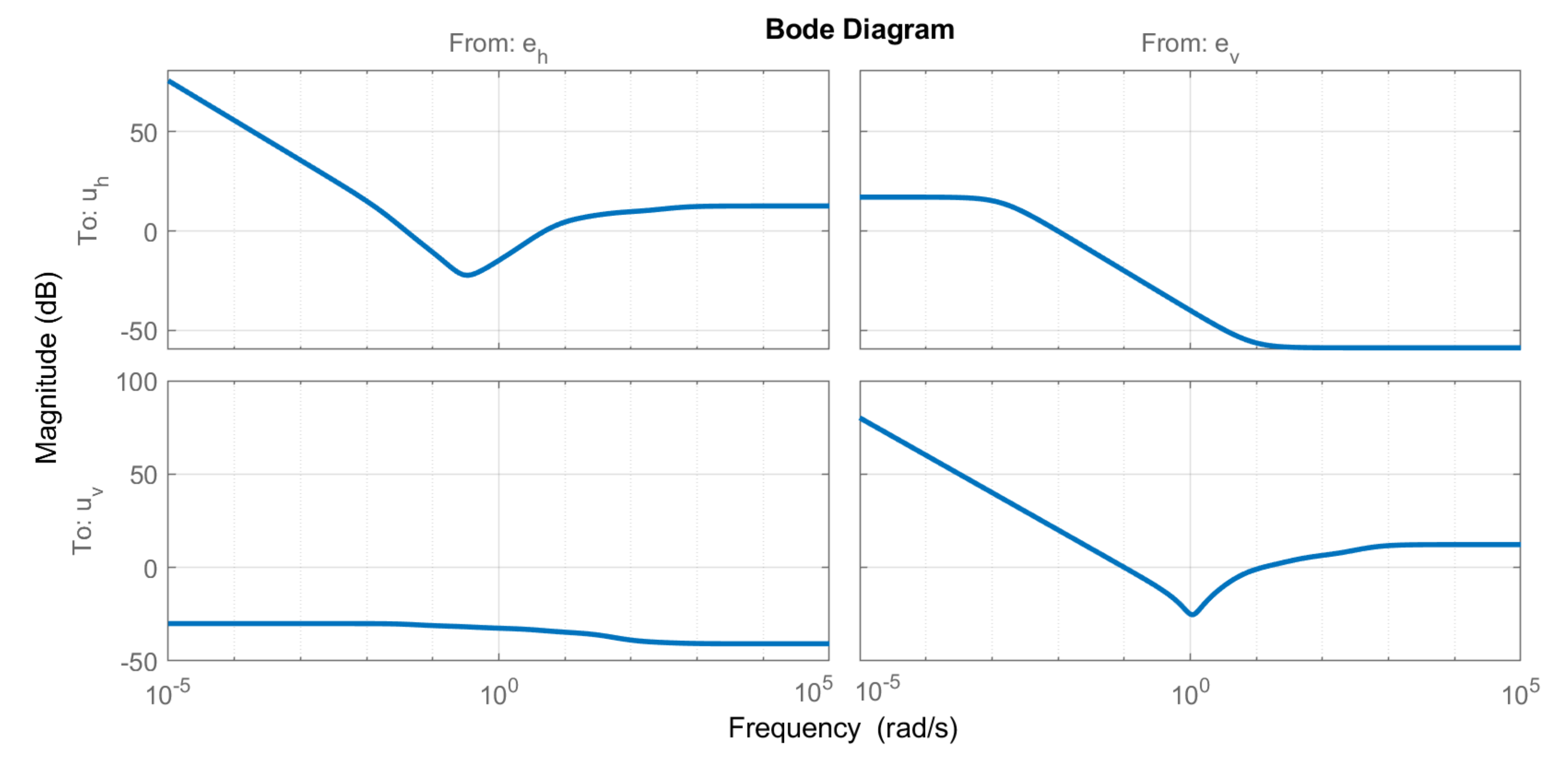
Figure 7. The nominal plant has been analyzed along with 100 Monte Carlo simulations for the given uncertainty range. Also, in order to underline that the control problem has been successfully solved, the weighting functions are also depicted and it can be noticed that all the simulated functions are under the imposed thresholds. Additionally, the Bode magnitude characteristics of the resulting controller are provided in
Figure 8.
The time-domain performance of the lower linear fractional transform between the linearized plant and the controller are presented using a step response in
Figure 9. In a similar manner, the nominal plant is illustrated along with 100 Monte Carlo simulations. The rise time for the azimuth position varies between
[s] and
[s], having a settling time between
[s] and
[s] and an overshoot between
and
, with no steady-state error. Similarly, the rise time for the pitch position is between
[s] and
[s], having a settling time between
[s] and 19 [s], with no overshoot and no steady-state error.
Numerical results will further be compared with the experimental results. The first set of experiments, shown in
Figure 10, have been made for a square reference with an amplitude of
[rad] and a period of 100 [s] for both axes. The initial conditions were varied in practice in order to illustrate the capability of the method. It can be noticed that for the azimuth position, the practical overshoot is a bit higher than in the linear case, with a comparable settling time and near-zero steady-state error due to the quantization effects. The pitch position presents overshoot for the initial step, while for the second step the behavior is similar to that of the linear system, with no overshoot, no steady-state error and comparable settling time.
The second set of experiments are made for the stabilization problem, where the reference for both axes is
[rad]. It can be noticed that the azimuth position presents an initial overshoot comparable to that obtained for the linear system, while the second part of the oscillation is more aggressive, underling the influence of the nonlinear components. In a similar manner, the pitch position presents an overshoot along with several oscillations, while the settling time is comparable with the linear case’s. The experimental results are shown in
Figure 11. Moreover, three different disturbances have been applied after 50 [s]: a perturbation on the vertical axis which leads the pitch position at the maximum value (blue), a perturbation on the horizontal axis with the same characteristics (cyan), and another small perturbation on the horizontal axis (black). It can be noticed that all disturbances have been successfully rejected.
Finally, the third set of experiments, depicted in
Figure 12, illustrates the behaviour of the proposed method for an operating point far from the forced equilibrium point used in the linearization procedure and controller synthesis. As such, a step of
[rad] has been initially applied, with a different pair
[rad] applied at the moment
[s]. For the horizontal axis, the overshoot is a bit higher than in the linear case, but with similar settling time and no steady-state error. Also, for the vertical axis, the overshoot is negligible for the first step and zero for the second step, having comparable settling times and no steady-state error. Therefore, the controller can be used for other operating points.
5. Discussion
In order to compare the current iteration of FO-PID
-synthesis with previous methods, the fixed-structure part of the
-synthesis mixed-sensitivity loop shaping control problem (
25) is solved using the artificial bee colony (ABC) approach presented in [
17]. The hyperparameters used for this experiment are: the swarm dimension
, the maximum number of ABC cycles 50, the maximum number of cycles with no improvements 10, the limit for the abandonment counter 10, the maximum number of
D–
K iterations 10, the maximum window length for assessing lack of progress 4, while the parameters for the cost functions are
and
. Using this setup, the fixed-structure mixed-sensitivity loop shaping
-synthesis problem (
25) is solved using five
D–-
K iterations. The resulting controller is:
Additionally, an experiment with unstructured
-synthesis has also been performed, leading to an upper bound of the structured singular value of
and a controller of 34th order, which means that robust stability and robust performance are not guaranteed, with the controller additionally of high order. The optimization algorithm has been stopped after three iterations because the diverging stopping criteria has been reached. A summary of the obtained results with the proposed method, the ABC method [
17] and the unstructured
-synthesis is presented in
Table 3.
As such, the unstructured version of the
-synthesis control problem could not be solved, resulting a high-order controller which does not guarantee robust stability and performance. On the other hand, both remaining methods managed to solve the control problem described in (
25). The new method introduced in this paper manages to solve the problem faster due to the advantages of the nonsmooth optimization techniques implemented in MATLAB.
As a future iteration, we propose to find a decentralized controller having a nonlinear component and a linear and time-invariant (LTI) robust component. The nonlinear component needs to be designed such that the lower linear fractional transform interconnection between the plant and such a component is asymptotically stable, as in [
28], where the passivity-based control framework has been extended for quasi-linear input-affine systems. Additionally, the LTI robust controller can be designed using the proposed method, the decentralized controller managing to ensure robust stability and performance for the nonlinear system. Moreover, the fractional-order element can be approximated using the presented ORA method only for
, with
. As such, another research direction is to find a method to integrate all positive values of
. On the other hand, the presented methods were considered in the continuous-time domain, although, for practical implementation, the controller must be discretized and also quantized. A starting point for this aspect could be the work presented in [
24].


