Brownian Behavior in Coupled Chaotic Oscillators

Abstract

Since the dynamical behavior of chaotic and stochastic systems is very similar, it is sometimes difficult to determine the nature of the movement. One of the best-studied stochastic processes is Brownian motion, a random walk that accurately describes many phenomena that occur in nature, including quantum mechanics. In this paper, we propose an approach that allows us to analyze chaotic dynamics using the Langevin equation describing dynamics of the phase difference between identical coupled chaotic oscillators. The time evolution of this phase difference can be explained by the biased Brownian motion, which is accepted in quantum mechanics for modeling thermal phenomena. Using a deterministic model based on chaotic Rössler oscillators, we are able to reproduce a similar time evolution for the phase difference. We show how the phenomenon of intermittent phase synchronization can be explained in terms of both stochastic and deterministic models. In addition, the existence of phase multistability in the phase synchronization regime is demonstrated.

1. Introduction

Brownian motion is the random motion of particles in a fluid medium as a result of collisions with fluid molecules. This transport phenomenon was named after the Scottish biologist Robert Brown, who in 1827 observed through a microscope how particles are retained in cavities inside a pollen grain in water. Although this discovery of Brownian motion was remarkable, the mechanisms causing this motion had not been identified. Later, Einstein and Smolowski, in their famous papers of 1905 and 1906, respectively [1,2], linked molecular kinetic theory to Brownian motion. Their theory was experimentally verified by French physicist Jean Baptiste Perrin, who established that Brownian motion in liquids is caused by the movement of molecules, and thus convincingly proved the existence of molecules and atoms.

Brownian motion is among the simplest random processes and is akin to two other simpler and more complex stochastic processes: random walk and Donsker’s theorem [3]. This universality is closely related to the versality of the normal distribution. In both cases, the use of normal distribution is often associated with mathematical convenience rather than model accuracy. Despite the great progress in understanding the nature of Brownian motion, many aspects remain unclear, and questions remain unanswered, for example, how this process depends on the interaction of particles with the environment, whether it is stochastic or deterministic, etc.

In mathematics, Brownian motion is interpreted as a Wiener process named after Norbert Wiener. This continuous random process is often used in various differential equations to describe physical phenomena that are affected by noise. In many cases, the quantum nature of equations requires a proper understanding of this process [4]. In chaos theory, the question of whether Brownian motion is stochastic or deterministic is rather philosophical. Although the equations describing chaotic phenomena are deterministic, it is inherently difficult to determine the initial conditions or parameters that govern the chaotic dynamical system with sufficient accuracy to replicate the exact same experiment in the laboratory without considering environmental noise. In recent decades, with the advent of computers, the scientific community has discovered that chaotic systems behave like stochastic ones when we perform simulations in which we can control the accuracy of parameters and initial conditions [5]. This brings us back to the philosophical question of what behavior in nature is truly random.

It is now well known that coupled chaotic oscillators, similar to limit cycles, can exhibit coherence phenomena [6]. One such phenomenon is phase synchronization, which is usually characterized by the phase difference between oscillators. Over the past few years, in articles devoted to chaotic phase synchronization, the authors reported that the phase difference between chaotic oscillator fluctuations in time, is like Brownian behavior [7,8].

In this paper, we explore the possibility of simulating the synchronous dynamics of coupled chaotic oscillators with stochastic differential equations, although it is not at all obvious that random behavior can be reproduced using deterministic equations. To do this, we consider a stochastic model and describe the biased Brownian motion in the same way as it was done in the framework of quantum mechanics. We show that the parameters governing such a system can be derived by studying the random motion trajectories. We then demonstrate that the phase difference between two coupled chaotic oscillators behaves like a trajectory derived from the stochastic model, and that parameters obtained with this model can be used to describe the chaotic behavior of the phase difference.

2. Stochastic Model

The simplest chaotic dynamical systems are usually described by ordinary differential equations that model nonlinear oscillators with noticeable fluctuations in amplitude and frequency. Systems of this type often have periodic solutions under the influence of external noise. Hence, from a nonchaotic deterministic model, we can come to a stochastic model that exhibits generalized dynamics of simple chaotic oscillators. This is the case we discuss below.

2.1. Modified Kuramoto Model

One of the most common deterministic models which represents limit cycle synchronization is the Kuramoto model [9], defined by the phase time derivative of each limit cycle as

$$\frac{d{\varphi }_i}{dt}={\omega }_i+\frac{K}{N}\sum _{j=1}^{N}sin({\varphi }_j-{\varphi }_i),i=1\dots N,$$

(1)

where ${\omega }_i$ is the natural frequency of i-th limit cycle. Note that Equation (1) describes phase dynamics of a symmetric all-to-all network of N limit cycle oscillators coupled with strength $K>0$. In an asymmetric network, $K_{ij}$ is under the sum in Equation (1) and represents the coupling strength between each pair of limit cycles. If a pair of oscillators are not connected, then $K_{ij}=0$.

An important property of a chaotic oscillator is the unpredictability of amplitude fluctuations. To describe these fluctuations in the Kuramoto model, we introduce a driving term $f(A_i)$, which takes into account the frequency dependence of the amplitude. We can now derive the modified Kuramoto model for an asymmetric network with a frequency-dependent amplitude, as follows

$$\frac{d{\varphi }_i}{dt}={\omega }_i+\frac{1}{N}\sum _{j=1}^N{K}_{ij}sin({\varphi }_j-{\varphi }_i)+f(A_i),i=1\dots N.$$

2.2. Langevin Dynamics of Two Coupled Chaotic Oscillators

Synchronization of coupled oscillators is often characterized by their phase difference $\theta ={\varphi }_2-{\varphi }_1$. Consider now a pair of unidirectionally coupled chaotic oscillators such that $K_{12}=0$ and $K_{21}=\kappa$. Then, two differential equations which govern their dynamics can be written as follows

$$\begin{array}{ccc}\hfill \frac{d{\varphi }_1}{dt}& =& {\omega }_1+f(A_1),\hfill \end{array}$$

(2a)

$$\begin{array}{ccc}\hfill \frac{d{\varphi }_2}{dt}& =& {\omega }_2+\frac{\kappa }{2}sin({\varphi }_1-{\varphi }_2)+f(A_2),\hfill \end{array}$$

(2b)

where Equations (2a) and (2b) represent respectively master and slave oscillators. Hence, the phase difference is given by

$$\frac{d\theta }{dt}=\Delta \omega -\frac{\kappa }{2}sin\theta +\xi (t),$$

(3)

where $\xi (t)=f(A_2)-f(A_1)$ is effective noise. For Langevin dynamics, the effective noise is a diffusive term, so that $\xi (t)=\sqrt{2D}w(t)$ (D being the diffusion coefficient and $w(t)$ is standard white noise).

In chaotic oscillators, the mean frequency of each isolated oscillator differs from the natural frequency due to nonlinearity. The mismatch between these two frequencies can be measured from the power spectrum of each oscillator, determining a maximum known as the dominant frequency (this effect will be discussed in the next section). We can now rewrite Equation (3) to obtain the following Langevin equation

$$\frac{d\theta }{dt}=\Delta \Omega -\frac{\kappa }{2}sin\theta +\sqrt{2D}w(t),$$

(4)

where $\Delta \Omega =〈{\Omega }_2-{\Omega }_1〉$ is the average mismatch between dominant frequencies of two chaotic oscillators [10]. The averaging is performed over the power spectra for different initial conditions, since we expect diffusion of the phase difference, and therefore it is nonergodic. It is easy to see that when the oscillators are identical and uncoupled, the average mismatch vanishes.

2.3. Mean Angular Velocity and Diffusion Coefficient

The time average of Equation (4) is calculated as

$$〈\frac{d\theta }{dt}〉=\underset{t\to \infty }{lim}\frac{1}{t}{\int }_0^t\frac{d\theta (\tau )}{d\tau }d\tau =\underset{t\to \infty }{lim}\frac{\theta (t)-\theta (0)}{t}.$$

(5)

Since standard white noise has a null expected value over time, in the ensemble sense the average of Equation (5) holds

$$\Delta \Omega =\underset{t\to \infty }{lim}\frac{〈\theta (t)-\theta (0)〉}{t},$$

(6)

where $〈·〉$ means the ensemble average. Then, $\Delta \Omega$ is the mean angular velocity of the Langevin Equation (4).

Taking into account Equation (6), the variance of $\theta (t)$ can be defined as

$${\sigma }^2(t)=〈{(\theta (t)-\theta (0)-\Delta \Omega t)}^2〉,$$

(7)

where $〈·〉$ is also the ensemble average. For a normal diffusion process [11], when $t\to \infty$ the variance is expected to be linear matching ${\sigma }^2=2D{t}^{\alpha }$ with $\alpha =1$, thus

$$D=\frac{1}{2}\underset{t\to \infty }{lim}\frac{〈{(\theta (t)-\theta (0)-\Delta \Omega t)}^2〉}{t}.$$

3. Deterministic Model

Consider two identical Rössler oscillators with diffusive unidirectional coupling. The system dynamics is modelled by the following equations

$$\begin{array}{ccc}\hfill \dot{x_1}& =& -{\omega }_1{y}_1-z_1,\hfill \\ \hfill \dot{y_1}& =& {\omega }_1{x}_1+a{y}_1,\hfill \\ \hfill \dot{z_1}& =& b+z_1(x_1-c);\hfill \\ \hfill \end{array}$$

(8a)

$$\begin{array}{ccc}\hfill \dot{x_2}& =& -{\omega }_2{y}_2-z_2,\hfill \\ \hfill \dot{y_2}& =& {\omega }_2{x}_2+a{y}_2+\kappa (y_1-y_2),\hfill \\ \hfill \dot{z_2}& =& b+z_2(x_2-c),\hfill \end{array}$$

(8b)

where $a=0.165$, $b=0.2$, $c=10$, and ${\omega }_1={\omega }_2=1$ are fixed parameters resulting in a chaotic regime. Equations (8a) and (8b) describe respectively the chaotic behavior of the master and slave oscillators. Since the oscillators are identical, they have the same natural frequency. Thus, when the coupling strength parameter $\kappa$ vanishes, they oscillate with the same dominant frequency. Due to nonlinearity, the natural and dominant frequencies do not match.

If a small mismatch exists between natural frequencies, the phenomenon of phase synchronization can be observed [7,12,13,14,15]. When the coupling strength is very small, the phase difference fluctuates as a random walk [8].

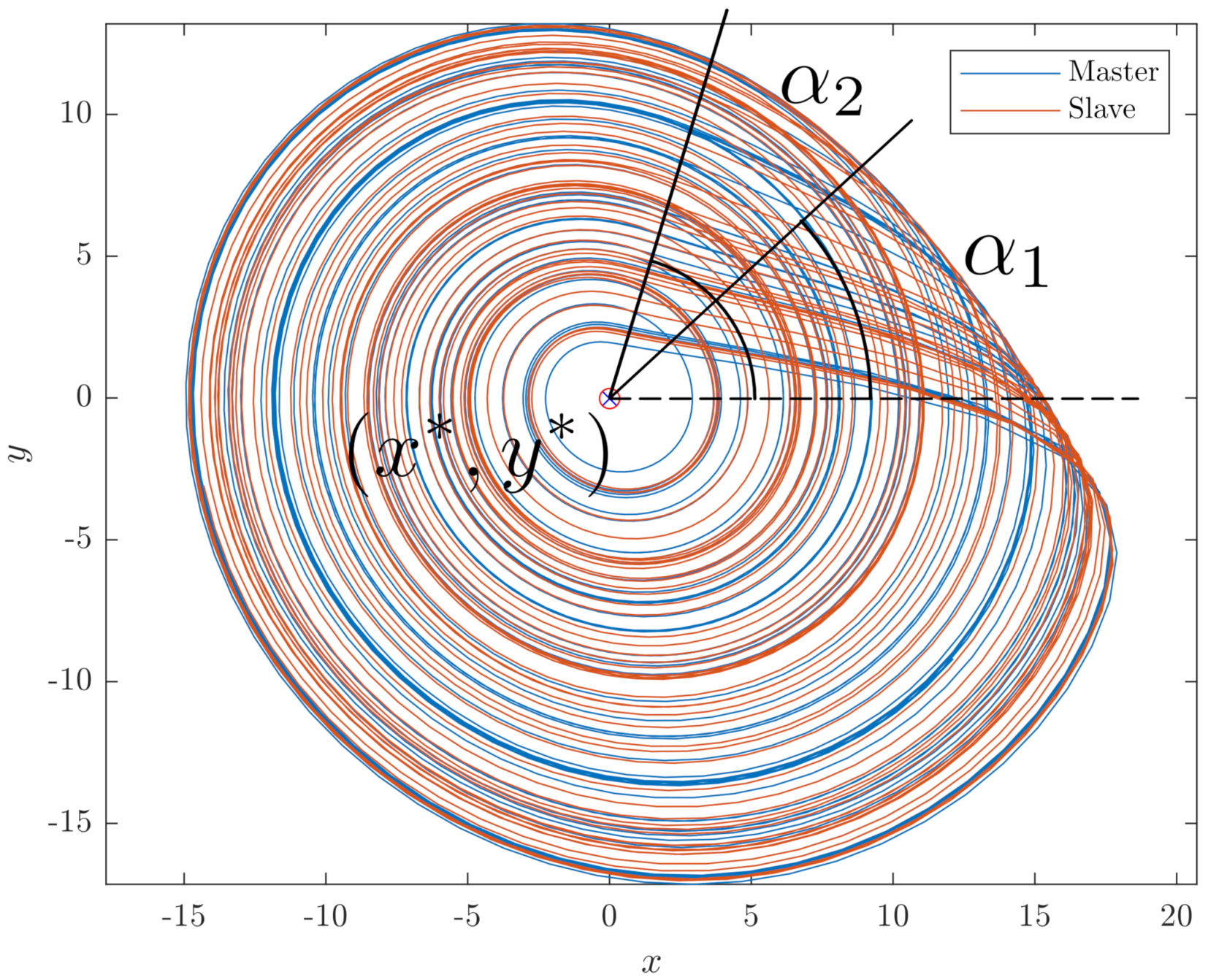
3.1. Chaotic Phase Difference

Since the Rössler attractor has a spiral shape, the phase of each oscillator can be calculated using the time series [16]. In projection on the ($x,y$) plane (see Figure 1), the position vector forms with the positive part of the $x^{\prime }$ axis the following relative phase

$$\alpha (t)=arctan\frac{y(t)-y^{*}}{x(t)-x^{*}},$$

(9)

where $arctan(·)\in \left[-\pi ,\pi \right)$ and ($x^{\prime },y^{\prime }$) are the Cartesian axes parallel to the ($x,y$) axes, in which the origin $(x^{*},y^{*})$ is the attractor center.

The relative phase is bounded and exhibits a jump every time a revolution is completed. To calculate the phase difference, we must first compute the absolute phase of each oscillator. To do this, we unwrap radian phases by replacing absolute jumps greater than $\pi$ to their $2\pi$ complement. Therefore, the absolute phase is $\varphi (t)={\bigcup }_k{\varphi }^k(t)$, where

$${\varphi }^k(t)=2\pi k+\alpha (t),t_k\le t<t_{k+1},$$

and $t_k$ occurs when $y(t_k)=y^{*}$ and $x(t_k)<x^{*}$ with $k\in {\mathbb{N}}_0$. Since the Rössler oscillator rotates counterclockwise, we consider $\varphi (t)$ as a continuous increasing function.

Linearizing the entire system in Equation (8) allows us to find the coordinates of the center of each attractor. Since the locations of two centers coincide and are independent of the coupling strength $\kappa$, we can now calculate the phase difference as $\theta (t)={\varphi }_2(t)-{\varphi }_1(t)$.

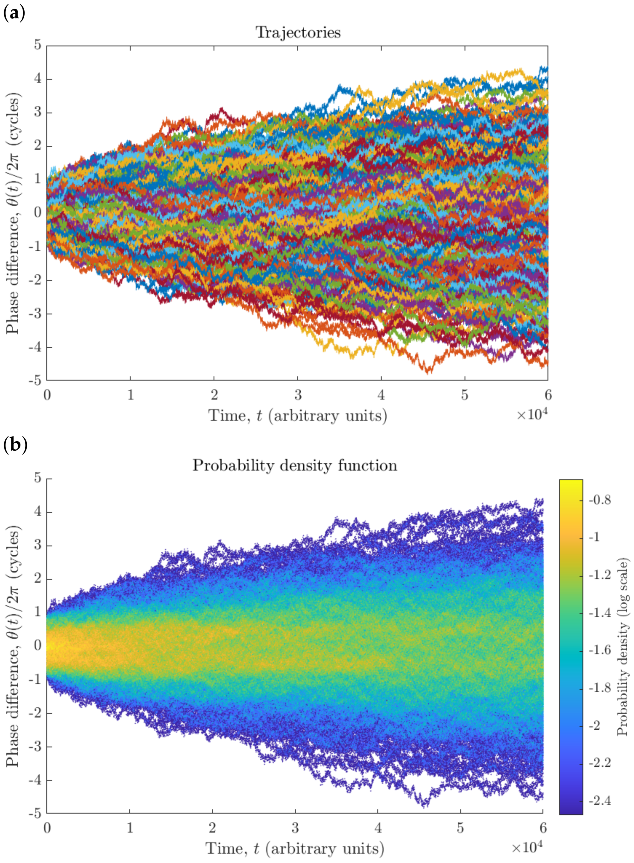
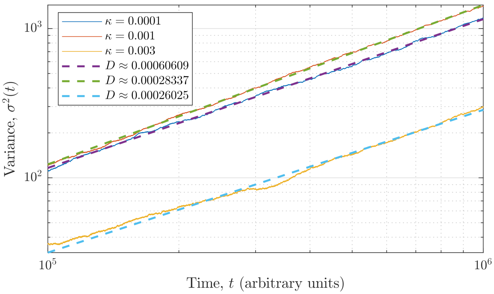
3.2. Brownian-like Phase Diffusion

With the intention of studying the phase difference diffusion, we carry out numerical simulations using the fifth-order Runge–Kutta method to obtain the time series of Equation (8) for various random initial conditions. We can obtain phase synchronization when the coupling strength exceeds a certain threshold value ($\kappa >{\kappa }_{th}$). In the phase synchronization regime, the phase difference fluctuates around a certain fixed value. Whereas for the coupling strength below the threshold, the phase difference changes linearly with time or switches to $2\pi$ radians.

The phase difference fluctuation looks like a random process similar to Brownian motion. In order to characterize this behavior, we compute probability density functions (PDF) [17] and mean power spectral densities (PSD) for the set of trajectories initiated from random initial conditions. Now, we consider the phase difference evolution for different values of the coupling strength $\kappa$.

When the oscillators are uncoupled ($\kappa =0$), there is no interaction between them. As seen from Figure 2, both the phase difference and the corresponding PDF increase or decrease in time depending on the initial conditions.

For weakly coupled oscillators, when the coupling strength is below the phase synchronization threshold ($\kappa <{\kappa }_{th}$), all phase difference trajectories gradually increase in time regardless of initial conditions, as seen from Figure 3a. At the same time, the PDF reveals intermittent phase locking, represented by high probability bands, multiples of $2\pi$ (Figure 3b). This phenomenon is detected for all values of the coupling strength below the phase synchronization threshold.

Brownian motion is characterized by a $\beta \approx -2$ power low of the mean PSD [18]. To check how close the observed phase difference is to Brownian motion PSD, we calculate $log〈S(\omega )〉$ ($S(\omega )$ being the PSD of $\theta (t)$ for each random initial condition) versus $log\omega$. The results displayed in Figure 4 confirm the Brownian-like behavior of our deterministic system.

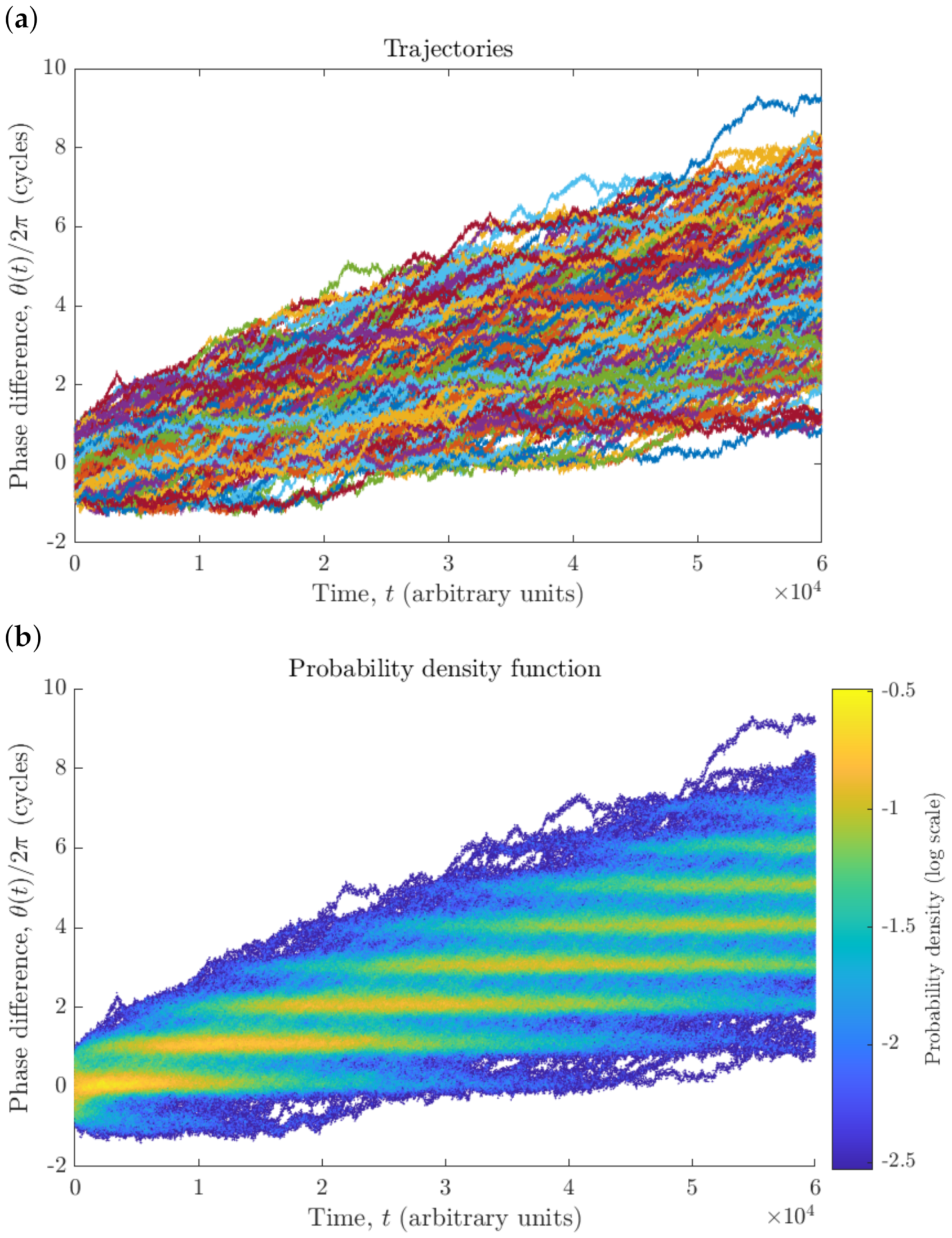
4. Biased Brownian Motion

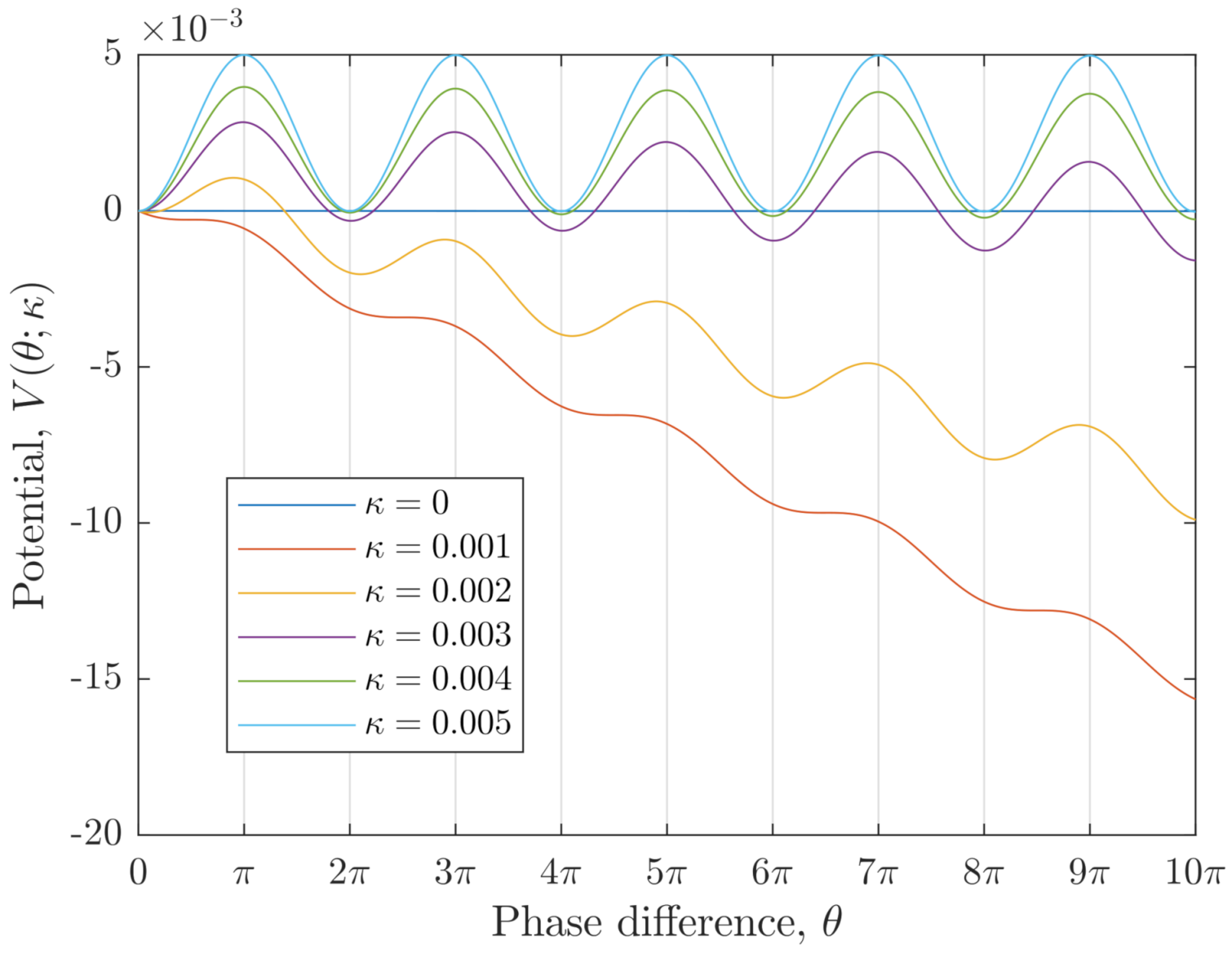
4.1. Matching Both Models

The phase drift shown in Figure 2 and Figure 3 can be computed with Equation (6). Specifically, the drift in the deterministic model is the mean angular velocity $\Delta \Omega$ which can be calculated as a slope of the time evolution of the average mismatch between dominant frequencies $〈\theta (t)-\theta (0)〉$ (see Equation (6) and Figure 5).

To find the diffusion coefficient D, we plot in Figure 6 the variance calculated with Equation (7) and fit this time dependence by a straight line. The slope of this dependence in a log scale is always near 1, that means normal diffusion, and the ordinate at the origin is the diffusion coefficient.

Figure 7 shows the variation of the diffusion coefficient and mean angular velocity with respect to the coupling strength. When D and $\Delta \Omega$ vanish, phase synchronization is achieved. We can also compare the variation of $\Delta \Omega$ computed by locating the dominant frequency in the power spectrum of each oscillator.

4.2. Itô-Langevin Form

Equation (4) can be transformed into the Itô–Langevin [19] form as follows

$$d{\Theta }_t=\left(\Delta \Omega (\kappa )-\frac{\kappa }{2}sin{\Theta }_t\right)dt+\sqrt{2D}d{W}_t,$$

(10)

where $W_t$ is the standard Wiener process such that $d{W}_t/dt=w(t)$.

The physical interpretation of Equation (4) is a random walk of a particle in a one-dimensional potential [20] and the deterministic force can be written as

$$-\frac{dV}{d\theta }=\Delta \Omega -\frac{\kappa }{2}sin\theta .$$

So, the stochastic differential Equation (10) is the Itô diffusion for a biased Brownian motion ${\Theta }_t$ in the tilted periodic potential

$$\begin{array}{ccc}\hfill V(\theta ;\kappa )& =& -\Delta \Omega (\kappa )\theta +\frac{\kappa }{2}{\int }^{\theta }sin\theta d\theta \hfill \\ & =& \frac{\kappa }{2}(1-cos\theta )-\Delta \Omega (\kappa )\theta .\hfill \end{array}$$

Some potentials are plotted in Figure 8 employing the values of $\Delta \Omega (\kappa )$ calculated in Section 4.1.

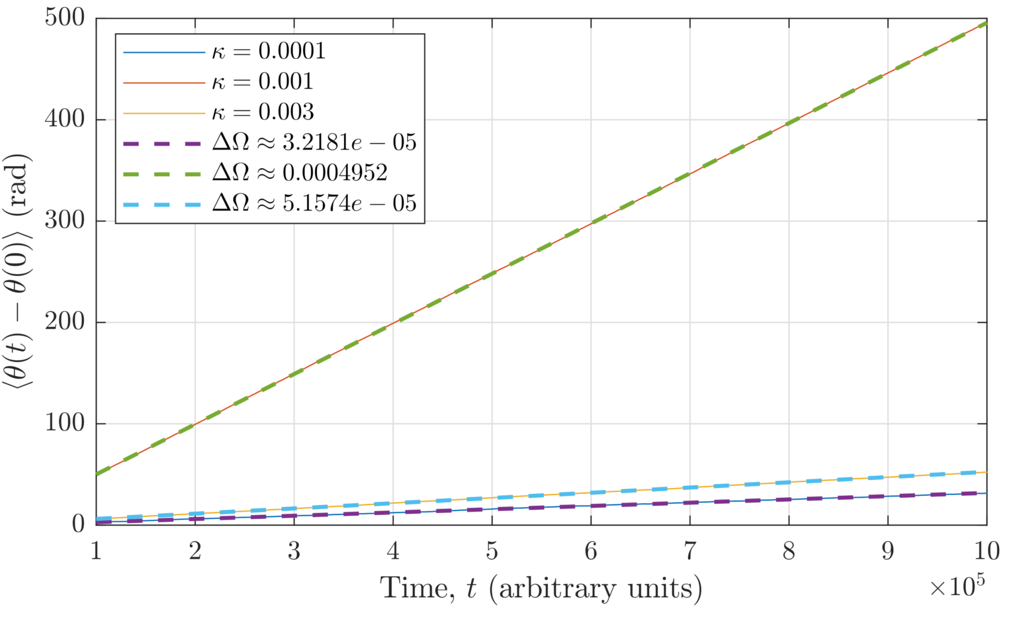
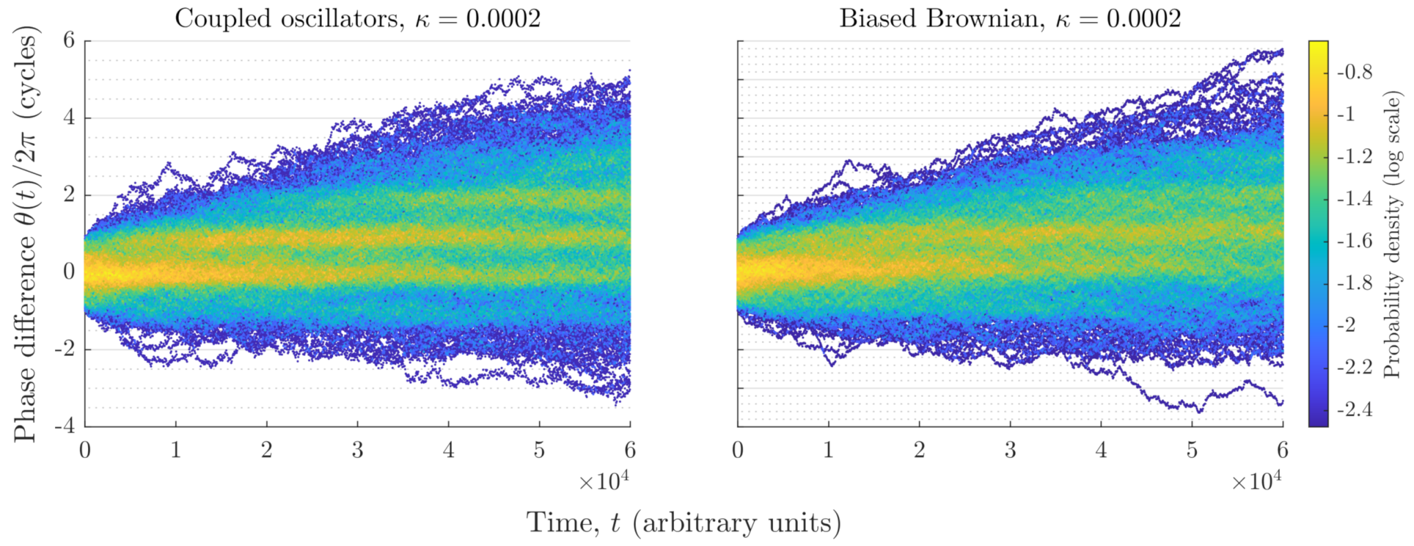
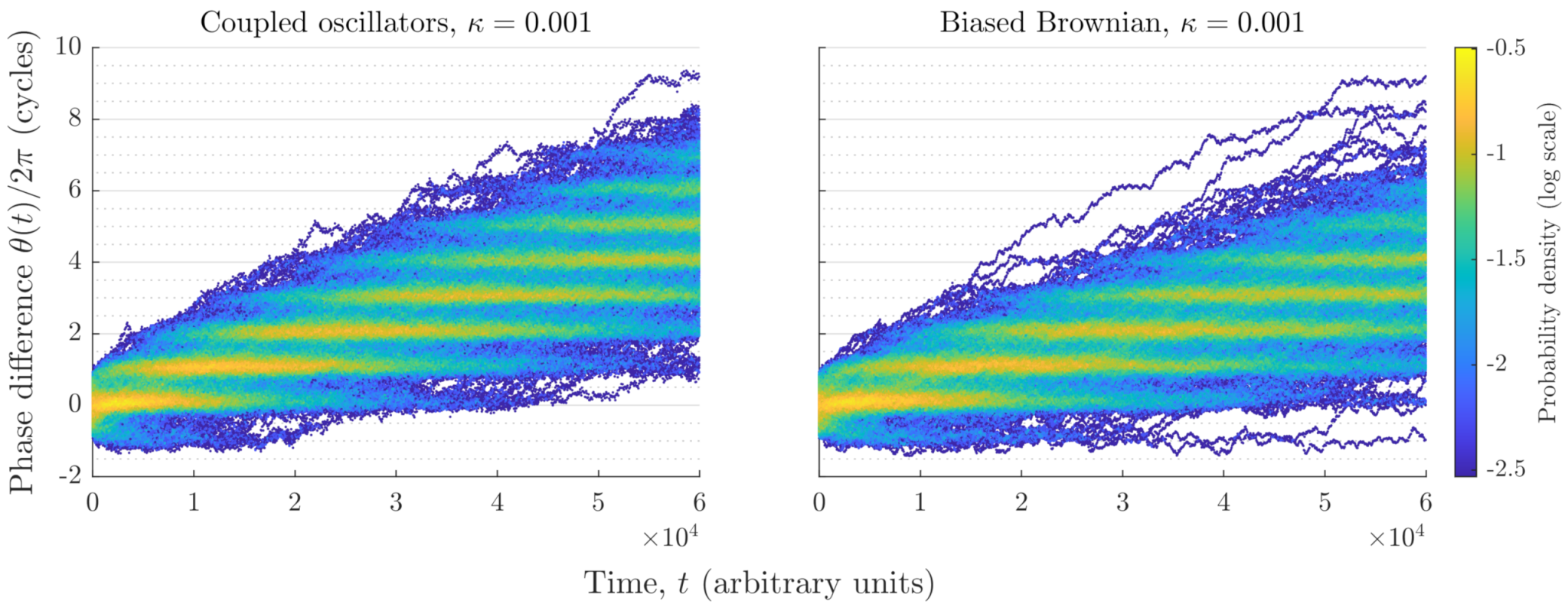
4.3. Numerical Simulations

Searching analytical solutions of stochastic equations is not an easy task. Although there are some approaches to find them (see, for example, [21]), it is not the aim of the present work. In this paper, we mainly focus on numerical simulations of Equation (10).

The variation in the diffusion coefficient $D(\kappa )$ shown in Figure 7 is due to the variation of the potential $V(\theta ;\kappa )$. So, in Equation (10) we set $D=D(\kappa =0)$ because it yields the value of the diffusion coefficient when there is no interaction, that is, $V(\theta )=0$.

To solve Equation (10), we apply the Euler–Maruyama method as follows

$${\Theta }_{j+1}={\Theta }_j+\gamma \left(\Delta \Omega (\kappa )-\frac{\kappa }{2}sin{\Theta }_j\right)+\sqrt{2D\gamma }\delta W_j,$$

where $\gamma >0$ is the step size and ${\left\{\delta W_j\right\}}_{j\in {\mathbb{N}}_0}\sim \mathcal{N}(0,1)$. In our simulations, we set ${\Theta }_0=\theta (0)$, that is, we choose the initial conditions as in the last section, and the step size $\gamma$ is the mean time between local extrema from deterministic trajectories.

In Figure 9, Figure 10 and Figure 11 we compare the probability density functions between simulations performed with the deterministic and stochastic models. One can see that the biased Brownian motion is a faithful representation of the deterministic model not only for the asynchronous regime, but even for coupling strength values corresponding to the phase synchronization regime.

Another interesting phenomenon which exhibits this system is the coexistence of three attractors, as seen from Figure 11, where three branches correspond to different initial conditions. This is the manifestation of phase multistability [22,23].

5. Conclusions

In this paper, we have analyzed the dynamics of two unidirectionally coupled chaotic oscillators with identical natural frequencies using a quantum mechanics approach. Nonlinearity in the basic equations leads to an increase in the oscillation frequency of the slave oscillator if the oscillators are not synchronized. This, in turn, increases the system randomness, as seen in Figure 7. In addition, the diffusion coefficient increases with increasing mean angular frequency. This phenomenon is contrary to common sense, since an increase in coherence between oscillators is usually expected when the oscillators are coupled. We suspect that when the mean angular velocity is higher, there is some kind of resonance between the harmonics of both oscillators at low frequencies, so that the trajectory of one of the oscillators will act as a “chaotic stationary wave” with respect to the trajectory of the other oscillator. Thus, the phase difference would be greater or less than at lower values of the mean angular velocity.

In addition, as shown in Figure 9 and Figure 10, intermittent phase synchronization occurs in the asynchronous regime. This phenomenon was revealed when studying the probability density of the phase difference. The stochastic model showed that some kind of force acts in this direction, which becomes stronger as the coupling strength is increased. Thus, the biased Brownian motion in an inclined potential, observed in quantum mechanics, reproduces the dynamics of the chaotic deterministic system.

Finally, we observed phase multistability in the weakly phase synchronized chaotic system, which manifested itself in the coexistence of attractors with different phase differences, shifted by $2\pi$.

References

1. Einstein, A. Über die von der molekularkinetischen theorie der wärme geforderte bewegung von in ruhenden flüssigkeiten suspendierten teilchen. Ann. Der Phys. 1905, 322, 549–560. [Google Scholar] [CrossRef] [Green Version]
2. von Smoluchowski, M. Zur kinetischen theorie der Brownschen molekularbewegung und der suspensionen. Ann. Der Phys. 1906, 326, 756–780. [Google Scholar] [CrossRef] [Green Version]
3. Donsker, M.D. Justification and extension of Doob’s heuristic approach to the Kolmogorov- Smirnov theorems. Ann. Math. Stat. 1952, 23, 277–281. [Google Scholar] [CrossRef]
4. Fisher, M.P.A.; Zwerger, W. Quantum Brownian motion in a periodic potential. Phys. Rev. B 1985, 32, 6190–6206. [Google Scholar] [CrossRef] [PubMed]
5. Huerta-Cuellar, G.; Jiménez-López, E.; Campos-Cantón, E.; Pisarchik, A.N. An approach to generate deterministic Brownian motion. Commun. Nonlinear Sci. Numer. Simul. 2014, 19, 2740–2746. [Google Scholar] [CrossRef]
6. Pikovsky, A.; Kurths, J.; Rosenblum, M.; Kurths, J. Synchronization: A Universal Concept in Nonlinear Sciences; Cambridge University Press: Cambridge, UK, 2003. [Google Scholar]
7. Pazó, D.; Mariño, I.P.; Pérez-Villar, V.; Pérez-Muñuzuri, V. Transition to chaotic phase synchronization through random phase jumps. Int. J. Bifurc. Chaos 2000, 10, 2533–2539. [Google Scholar] [CrossRef] [Green Version]
8. Pisarchik, A.N.; Huerta-Cuellar, G.; Kulp, C.W. Statistical analysis of symbolic dynamics in weakly coupled chaotic oscillators. Commun. Nonlinear Sci. Numer. Simul. 2018, 62, 134–145. [Google Scholar] [CrossRef]
9. Kuramoto, Y. International symposium on mathematical problems in theoretical physics. Lect. Notes Phys. 1975, 30, 420. [Google Scholar]
10. Zakharova, A.S.; Vadivasova, T.E.; Anishchenko, V.S. Spectral-correlation analysis of coupled chaotic self-sustained oscillators. Int. J. Bifurc. Chaos 2008, 18, 2877–2882. [Google Scholar] [CrossRef]
11. Kubo, R.; Toda, M.; Hashitsume, N. Statistical Physics II: Nonequilibrium Statistical Mechanics; Springer Science & Business Media: Berlin, Germany, 2012. [Google Scholar]
12. Fujisaka, H.; Yamada, T.; Kinoshita, G.; Kono, T. Chaotic phase synchronization and phase diffusion. Phys. D Nonlinear Phenom. 2005, 205, 41–47. [Google Scholar] [CrossRef]
13. Kye, W.H.; Lee, D.S.; Rim, S.; Kim, C.M.; Park, Y.J. Periodic phase synchronization in coupled chaotic oscillators. Phys. Rev. E 2003, 68, 025201. [Google Scholar] [CrossRef] [PubMed] [Green Version]
14. Pikovsky, A.; Rosenblum, M.; Kurths, J. Phase synchronization in regular and chaotic systems. Int. J. Bifurc. Chaos 2000, 10, 2291–2305. [Google Scholar] [CrossRef]
15. Rosenblum, M.G.; Pikovsky, A.S.; Kurths, J. Phase Synchronization of Chaotic Oscillators. Phys. Rev. Lett. 1996, 76, 1804–1807. [Google Scholar] [CrossRef] [PubMed]
16. Boccaletti, S.; Pisarchik, A.N.; Genio, C.I.D.; Amann, A. Synchronization: From Coupled Systems to Complex Networks; Cambridge University Press: Cambridge, UK, 2018. [Google Scholar]
17. Alves, S.B.; de Oliveira, G.F.; de Oliveira, L.C.; Passerat de Silans, T.; Chevrollier, M.; Oriá, M.; de, S.; Cavalcante, H.L.D. Characterization of diffusion processes: Normal and anomalous regimes. Phys. A Stat. Mech. Its Appl. 2016, 447, 392–401. [Google Scholar] [CrossRef]
18. Gaspard, P.; Briggs, M.E.; Francis, M.K.; Sengers, J.V.; Gammon, R.W.; Dorfman, J.R.; Calabrese, R.V. Experimental evidence for microscopic chaos. Nature 1998, 394, 865–868. [Google Scholar] [CrossRef]
19. Borland, L. Ito-Langevin equations within generalized thermostatistics. Phys. Lett. A 1998, 245, 67–72. [Google Scholar] [CrossRef]
20. Lindner, B.; Kostur, M.; Schimansky-Geier, L. Optimal diffusive transport in a tilted periodic potential. Fluct. Noise Lett. 2001, 1, R25–R39. [Google Scholar] [CrossRef]
21. Särkkä, S.; Solin, A. Applied Stochastic Differential Equations; Cambridge University Press: Cambridge, UK, 2019. [Google Scholar]
22. Pisarchik, A.N.; Feudel, U. Control of multistability. Phys. Rep. 2014, 540, 167–218. [Google Scholar] [CrossRef]
23. Shabunin, A.V. Phase multistability in a dynamical small world network. Chaos 2015, 25, 013109. [Google Scholar] [CrossRef] [PubMed]
Figure 1. Phase portraits of chaotic attractors of the master and slave Rössler oscillators. They both share the center coordinates ( x * , y * ) . The relative phase of each oscillator is represented by α 1 and α 2 angles calculated by Equation (9).
Mathematics 09 02503 g001
Figure 2. (a) Deterministic trajectories of phase difference θ ( t ) for random initial conditions and (b) corresponding probability density function, for coupling strength κ = 0 .
Mathematics 09 02503 g002
Figure 3. (a) Deterministic trajectories of phase difference θ ( t ) for random initial conditions and (b) corresponding probability density function, for coupling strength κ = 0.001 .
Mathematics 09 02503 g003
Figure 4. Averaged power spectral density from phase difference θ ( t ) for random initial conditions of the deterministic model with (a) κ = 0 and (b) κ = 0.001 .
Mathematics 09 02503 g004
Figure 5. Average mismatch between dominant frequencies for different values of coupling strength κ . The slope of the fitted straight lines are the mean angular velocities.
Mathematics 09 02503 g005
Figure 6. Logarithmic representation of variance σ 2 ( t ) for different values of κ . The ordinates at the origin of the fitted straight lines represent the diffusion coefficients D, while their slopes approximate to the unit indicating normal diffusion.
Mathematics 09 02503 g006
Figure 7. Diffusion coefficient D and mean angular velocity Δ Ω versus coupling strength κ calculated from the time series (blue circles) and from the averaged difference of dominant frequencies (orange triangles).
Mathematics 09 02503 g007
Figure 8. Potentials V ( θ ; κ ) for different values of coupling strength κ .
Mathematics 09 02503 g008
Figure 9. Probability density function of θ ( t ) over time for (left) deterministic and (right) stochastic ( Θ t ) models for κ = 0.0002 and the same initial conditions. Intermittent phase locking is present even for so small a coupling strength.
Mathematics 09 02503 g009
Figure 10. Probability density function of θ ( t ) over time for (left) deterministic and (right) stochastic ( Θ t ) models for κ = 0.001 and the same initial conditions. The randomness if higher than in the case of the uncoupled oscillators.
Mathematics 09 02503 g010
Figure 11. Probability density function of θ ( t ) over time for (left) deterministic and (right) stochastic ( Θ t ) models for κ = 0.01 and the same initial conditions. In the phase synchronization regime, both models exhibit confined Brownian-like motion. The three coexisting branches indicate underlying phase multistability.
Mathematics 09 02503 g011
Publisher’s Note: MDPI stays neutral with regard to jurisdictional claims in published maps and institutional affiliations.