1. Introduction
Definitions play a very important role in scientific and educational literature because they define the major concepts that are operated inside the text. Despite mathematical and generic definitions being pretty similar in their linguistic style (see the example of two definitions below: the first, defining ASCII, is general, while the second defines mathematical object), supervised identification of mathematical definitions benefits from a training on a mathematical domain, as we previously showed in [
1].
Definition 1. American Standard Code for Information Interchange, also called ASCII, is a character encoding based on English alphabet.
Definition 2. The magnitude of a number, also called its absolute value, is its distance from zero.
Naturally, we expect to find mathematical definitions in mathematical articles, which frequently use formulas and notations in both definitions and surrounding text. The number of words in mathematical text is smaller than in standard text due to the formulas that are used to express the former. The mere presence of formulas is not a good indicator of a definition sentence because the surrounding sentences may also use notations and formulas. As an example of such text, Definition 3, below, contains a definition from Wolfram MathWorld. Only the first sentence in this text is considered a definition sentence, even though other sentences also contain mathematical notations.
Definition 3. A finite field is a field with a finite field order (i.e., number of elements), also called a Galois field. The order of a finite field is always a prime or a power of a prime. For each prime power, there exists exactly one (with the usual caveat that "exactly one" means "exactly one up to an isomorphism") finite field , often written as in current usage.
Multiple current methods for automatic DE view it as a binary classification task, where a sentence is classified as a definition or a non-definition. A supervised learning process is usually applied for this task, employing feature engineering for sentence representation. However, all recently published works study generic definitions, without evaluation of their methods on mathematical texts.
In this paper, we describe a supervised learning method for automatic DE from both generic and mathematical texts. Our method applies ensemble learning to adjusted-by-oversampling data, where 12 deep neural network-based models are trained on a dataset with labeled definitions and then applied on test sentences. The final label of a sentence is decided by the ensemble voting.
Our method is evaluated on four different corpora; three for generic DE and one is an annotated corpus of mathematical definitions.
The main contributions of this paper are (1) the introduction of a new corpus of mathematical texts with annotated sentences and (2) an evaluation of an ensemble learning model for the DE task, (3) an evaluation of the introduced ensemble learning model on a general and mathematical domains, including (4) cross-domain experiments. We performed extensive experiments with different ensemble models on four datasets, including the introduced one. Our experiments demonstrate the superiority of our model for the three out of four datasets, belonging to two different domains. The paper is organized as follows.
Section 2 contains a survey of up-to-date related work.
Section 3 describes our approach.
Section 4 provides the evaluation results and their analysis. Finally,
Section 5 contains our conclusions.
2. Related Work
Definition extraction has been a popular topic in NLP research for more than a decade [
2], and it remains a challenging and popular task today as a recent research call at SemEval-2020 show. Prior work in the field of DE can be divided into three main categories: (1) rule-based methods, (2) machine-learning methods relying on manual feature engineering, and (3) methods that use deep learning techniques.
Early works about DE from text documents belong to the first category. These works rely mainly on manually crafted rules based on linguistic parameters. Klavans and Muresan [
3] presented the DEFINDER, a rule-based system that mines consumer-oriented full text articles to extract definitions and the terms they define; the system is evaluated on definitions from on-line dictionaries such as the UMLS Metathesaurus [
4]. Xu et al. [
2] used various linguistic tools to extract kernel facts for the definitional question-answering task in Text REtrieval Conference (TREC) 2003. Malaise et al. [
5] used semantic relations to mine defining expressions in domain-specific corpora, thus detecting semantic relations between the main terms in definitions. This work is evaluated on corpora from fields of anthropology and dietetics. Saggion and Gaizauskas [
6], Saggion [
7] employed analysis of on-line sources to find lists of relevant secondary terms that frequently occur together with the definiendum in definition-bearing passages. Storrer and Wellinghoff [
8] proposed a system that automatically detects and annotates definitions for technical terms in German text corpora. Their approach focuses on verbs that typically appear in definitions by specifying search patterns based on the valency frames of definitor verbs. Borg et al. [
9] extracted definitions from nontechnical texts using genetic programming to learn the typical linguistic forms of definitions and then using a genetic algorithm to learn the relative importance of these forms. Most of these methods suffer from both low recall and precision (below
), because definition sentences occur in highly variable and noisy syntactic structures.
The second category of DE algorithms relies on semi-supervised and supervised machine learning that use semantic and other features to extract definitions. This approach generates DE rules automatically but relies on feature engineering to do so. Fahmi and Bouma [
10] presented an approach to learning concept definitions from fully parsed text with a maximum entropy classifier incorporating various syntactic features; they tested this approach on a subcorpus of the Dutch version of Wikipedia. In [
11], a pattern-based glossary candidate detector, which is capable of extracting definitions in eight languages, was presented. Westerhout [
12] described a combined approach that first filters corpus with a definition-oriented grammar, and then applies machine learning to improve the results obtained with the grammar. The proposed algorithm was evaluated on a collection of Dutch texts about computing and e-learning. Navigli and Velardi [
13] used Word-Class Lattices (WCLs), a generalization of word lattices, to model textual definitions. The authors introduced a new dataset called WCL that was used for the experiments. They achieved a
F1 score on this dataset. Reiplinger et al. [
14] compared lexico-syntactic pattern bootstrapping and deep analysis. The manual rating experiment suggested that the concept of definition quality in a specialized domain is largely subjective, with a
agreement score between raters. The DefMiner system, proposed in [
15], used Conditional Random Fields (CRF) to predict the function of a word and to determine whether this word is a part of a definition. The system was evaluated on a W00 dataset [
15], which is a manually annotated subset of ACL Anthology Reference Corpus (ACL ARC) ontology. Boella and Di Caro [
16] proposed a technique that only uses syntactic dependencies between terms extracted with a syntactic parser and then transforms syntactic contexts to abstract representations to use a Support Vector Machine (SVM). Anke et al. [
17] proposed a weakly supervised bootstrapping approach for identifying textual definitions with higher linguistic variability. Anke and Saggion [
18] presented a supervised approach to DE in which only syntactic features derived from dependency relations are used.
Algorithms in the third category use Deep Learning (DL) techniques for DE, often incorporating syntactic features into the network structure. Li et al. [
19] used Long Short-Term Memory (LSTM) and word vectors to identify definitions and then tested this approach on the English and Chinese texts. Their method achieved a
F-measure on the WCL dataset. Anke and Schockaert [
20] combined Convolutional Neural Network (CNN) and LSTM, based on syntactic features and word vector representation of sentences. Their experiments showed the best F1 score (
) on the WCL dataset for CNN and the best F1 score (
) on the W00 dataset for the CNN and Bidirectional LSTM (BLSTM) combination, both with syntactically enriched sentence representation. Word embedding, when used as the input representation, have been shown to boost the performance in many NLP tasks, due to its ability to encode semantics. We believe that a choice to use word vectors as input representation in many DE works was motivated by its success in NLP-related classification tasks.
We use the approach of [
20] as a starting point and as a baseline for our method. We further extend this work by (1) additional syntactic knowledge in a sentence representation model, (2) testing additional network architectures, (3) combining 12 configurations (that were the result of different input representations and architectures) in a joint ensemble model, and (4) evaluation of the proposed methodology on a new dataset of mathematical texts. As previously shown in our and others’ works [
1,
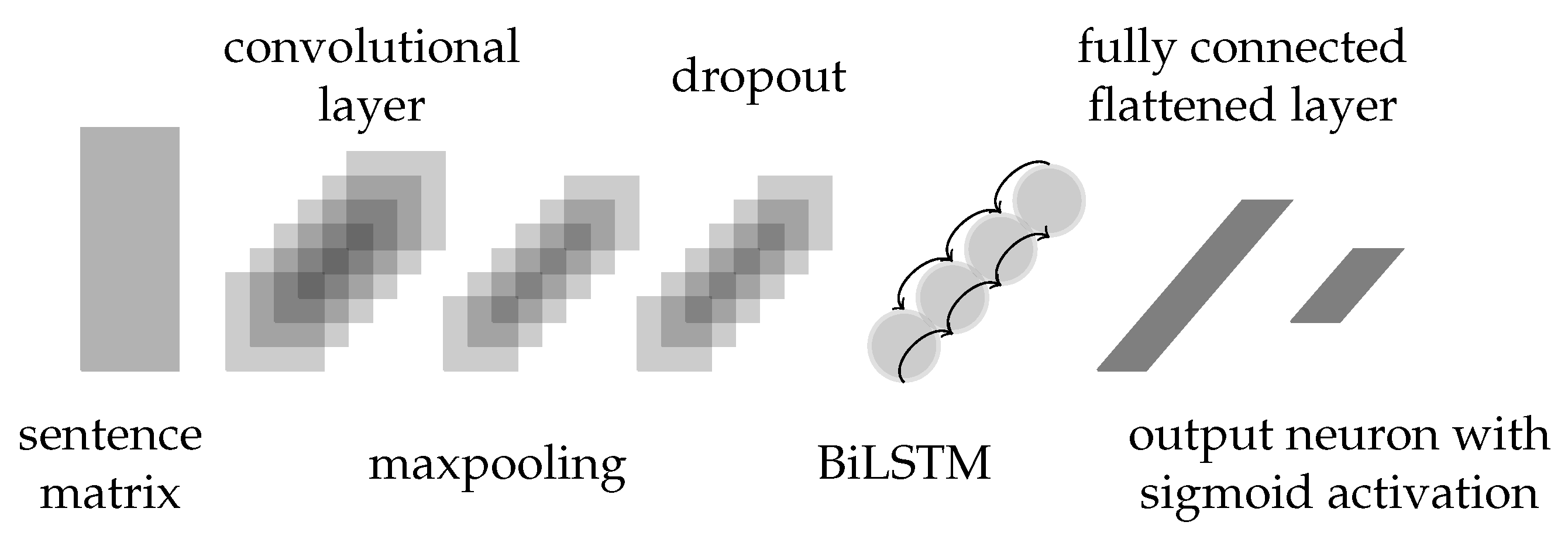
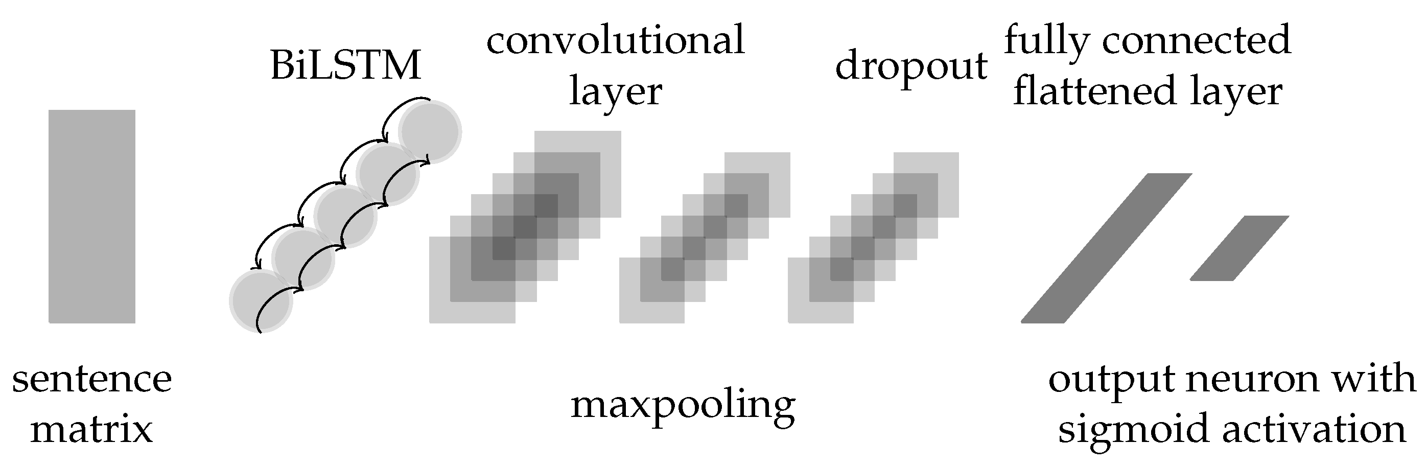
20], dependency parsing can add valuable features to the sentence representation in the DE task, including mathematical DE. The same works showed that a standard convolutional layer can be sufficiently applied to automatically extract the most significant features from the extended representation model, which improves accuracy for the classification task. Word embedding matrices enhanced with dependency information naturally call for CNN due to their size and CNN’s ability to decrease dimensionality swiftly. On the other hand, sentences are sequences for which LSTM is naturally suitable. In [
1], we explored how the order of the CNN and LSTM layers and the input representation affect the results. To do that, we evaluated and compared between 12 configurations (see
Section 3.3). As result, we obtained a conclusion that CNN and its combination with LSTM, applied on a syntactically enriched input representation, outperform other configurations. However, as we show in our experimental evaluation (see
Section 4), all the models individually are inferior to the ensemble approach.
Following recent research demonstrating the superiority of pretrained language models on many NLP tasks, including DE [
21,
22], we apply fine-tuned BERT [
23,
24] on our data and compare its results with the results of the proposed method.
4. Experiments
Our experiments aim at testing our hypothesis about superiority of the ensemble of all 12 composition models over single models and SOTA baselines.
Based on the feature analysis described in
Section 4.8, we decided to employ all 12 configurations as composition models and, based on the observations from our previous work [
1], we use pretrained fastText (further denoted by FT) word embedding in all of them.
Tests were performed on a cloud server with 32 GB of RAM, 150 GB of PAGE memory, an Intel Core I7-7500U 2.70 GHz CPU, and two NVIDIA GK210GL GPUs.
4.1. Tools
The models were implemented with help of the following tools: (1) Stanford CoreNLP wrapper [
27] for Python (tokenization, sentence boundary detection, and dependency parsing), (2) Keras [
28] with Tensorflow [
29] as a back-end (NN models), (3) fastText vectors pretrained on English webcrawl and Wikipedia [
26], (4) Scikit-Learn [
30] (evaluation with F1, recall, and precision metrics), (5) fine-tunable BERT python package [
24] available at
https://github.com/strongio/keras-elmo (accessed on 1 September 2021), and (6) WEKA software [
31]. All neural models were trained with batch size 32 and 10 epochs.
4.2. Datasets
In our work we use the following four datasets–DEFT, W00, WCL, and WFMALL–that are described below. The dataset domain, number of sentences for each class, majority vote values, total number of words, and number of words with non-zero fastText (denoted by FT) word vectors are given in
Table 1.
4.2.1. The WCL Dataset
The World-Class Lattices (WCL) dataset [
32] was introduced in [
33]. It is constructed from manually annotated Wikipedia articles in English. We used the WCL v1.2 version that contains 4719 annotated sentences, 1871 of which are proper definitions and 2847 are
distractor sentences that have similar structures with proper definitions, but are not actually definitions. This dataset focuses on generic definitions in various areas. A sample definition sentence from this dataset is
American Standard Code for Information Interchange (TARGET) is a character encoding based on English alphabet.
and a sample distractor is
The premise of the program revolves around TARGET, Parker an 18-year-old country girl who moves back and forth between her country family, who lives on a bayou houseboat, and the wealthy Brents, who own a plantation and pancake business.
WCL contains the following annotations: (1) the DEFINIENDUM field (DF), referring to the word being defined and its modifiers, (2) the DEFINITOR field (VF), referring to the verb phrase used to introduce a definition, (3) the DEFINIENS field (GF) which includes the genus phrase, and (4) the REST field (RF), which indicates all additional sentence parts. According to the dataset description, existence of the first three fields indicates that a sentence is a definition.
4.2.2. The DEFT Dataset
The DEFT corpus, proposed in [
34], consists of annotated content from two different data sources: various 2017 SEC contract filings from the publicly available US Securities and Exchange Commission EDGAR (SEC) database, and sentences from the
https://cnx.org/ open source textbooks (accessed on 1 September 2021). The partial corpus is available for download from GitHub at
https://github.com/adobe-research/deft_corpus (accessed on 1 September 2021). We have used this part of the DEFT corpus in our experiments; it contains 562 definition sentences and 1156 non-definition sentences. A sample definition sentence from this dataset is
A hallucination is a perceptual experience that occurs in the absence of external stimulation.
and a sample non-definition sentence is
In monocots, petals usually number three or multiples of three; in dicots, the number of petals is four or five, or multiples of four and five.
4.2.3. The W00 Dataset
The W00 dataset [
35], introduced in [
15], was compiled from ACL ARC ontology [
36] and contains 2185 manually annotated sentences, with 731 definitions and 1454 non-definitions; the style of the distractors is different from the one used in the WCL dataset. A sample definition sentence from this dataset is
Our system, SNS (pronounced “essence”), retrieves documents to an unrestricted user query and summarizes a subset of them as selected by the user.
and a sample distractor is
The senses with the highest confidence scores are the senses that contribute the most to the function for the set.
Annotation of the W00 dataset is token-based, with each token in a sentence identified by a single label that indicates whether a token is a part of a term (T), a definition (D), or neither (O). According to the original annotation, a sentence is considered not to be a definition if all its tokens are marked as O. Sentence that contains tokens marked as T or D is considered to be a definition.
4.2.4. The WFMALL Dataset
The WFMALL dataset is an extension of the WFM dataset [
37], introduced by us in [
1]. It was created by us after collecting and processing all 2352 articles from Wolfram Mathworld [
38]. The final dataset contains 6140 sentences, of which 1934 are definitions and 4206 are non-definitions. Sentences were extracted automatically and then manually separated into two categories: definitions and statements (non-definitions). All annotators (five in total) have at least BSc degree and learned academic mathematical courses (research group members, including three research students). The data were semi-automatically segmented to sentences with Stanford CoreNLP package and then manually assessed. All malformed sentences (as result of wrong segmentation) were fixed, 116 very short sentences (with less than 3 words) were removed. All sentences related to Wolfram Language (
https://en.wikipedia.org/wiki/Wolfram_Language, accessed on 1 September 2021) were removed because they relate to a programming language and describe how mathematical objects are expressed in this language, and not how they are defined. Sentences with formulas only, without text, were also removed. The final dataset was split to nine portions, saved as Unicode text files. Three annotators worked on each portion. First, two annotators labeled sentences independently. Then, all sentences that were given different labels were finally annotated by the third annotator (controller) (We decided that a label with majority vote will be selected. Therefore, the third annotator (controller) labeled only the sentences with contradict labels.). The final label was set by majority vote. The Kappa agreement between annotators was 0.651, which is considered substantial agreement.
This dataset is freely available for download from GitHub (
https://drive.google.com/drive/folders/1052akYuxgc2kbHH8tkMw4ikBFafIW0tK?usp=sharing, accessed on 1 September 2021). A sample definition sentence from this dataset is
The -von Dyck group, also sometimes termed the-von Dyck group, is defined as the von Dyck groupwith parameters .
and a sample non-definition is
Any 2-Engel group must be a group of nilpotency class 3.
4.3. Evaluation Setup
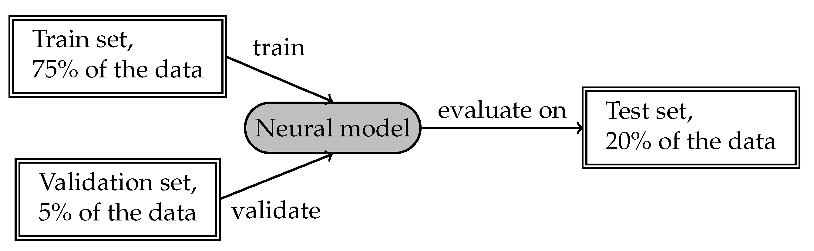
Datasets were oversampled with the ’minority’ setting, and split to the NN training set (70%), the NN validation set (5%), and the NN test set (25%). Then the labels of all 12 models on the NN test set were used to form the ensemble dataset, which was further split into the ensemble training set (5% of the original data size) and the ensemble test set (20% of the original data size). In this setting, we have a test set size identical to those of baselines that used 75% training, 5% validation, and 20% test set split.
For the consistency of the experiment, it was important to us to keep the same training and validation sets for individual models, whether as stand-alone or as composition models in an ensemble. Additionally, all evaluated and compared models, including ensemble, were evaluated on the same test set. Because ensemble models were trained using traditional machine-learning algorithms, no validation set was needed for them.
4.4. Text Preprocessing
Regarding all four datasets described above, we applied the same text preprocessing steps in the following manner:
Sentence splitting was derived explicitly from the datasets, without applying any additional procedure, in the following manner: DEFT, WCL, and W00 datasets came pre-split, and sentence splitting for the new WFMALL dataset was performed semi-automatically by our team (using Stanford CoreNLP SBD, followed by manual correction, due to many formulas in the text).
Tokenization and dependency parsing were performed on all sentences with the help of the Stanford CoreNLP package [
39].
For the W00 datasets used in [
20] for DE, we replaced parsing by SpaCy [
40] with the Stanford CoreNLP parser.
We applied fastText [
41] vectors pretrained on English webcrawl and Wikipedia (available at [
26]).
4.5. Baselines
We compared our results with five baselines:
DefMiner [
15], which uses Conditional Random Fields to detect definition words;
BERT [
23,
24], fine-tuned on the training subset of every dataset for the task of sentence classification;
CNN_LSTM
ml, proposed in [
20];
CNN_LSTMm, which is the top-ranked composition model on the adjusted WFMALL dataset.
CNN_LSTMmld, which is the top-ranked composition model on the adjusted W00 dataset.
We applied two supervised models for the ensemble voting: Linear Regression (LR) and Random Forest (RF). The results reported here are the average over 10 runs, with random reshuffling applied to the dataset each time (We did not apply a standard 10-fold cross validation due to a non-standard proportion between a training and a test dataset. Additionally, 10-fold cross validation was not applied on individual models, as it is not a standard evaluation technique for deep NNs.). We also applied the majority voting, denoted as Ensemble majority (Our code will be released once the paper is accepted).
4.6. Results for the Mathematical Domain
Table 2 contains the evaluation results (accuracy) for all systems on the WFMALL dataset, with bold font indicating the best scores. It can be seen that (1) oversampling improves performance of NN baselines and (2) all ensemble models outperform the baseline systems and all the individual NN models.
4.7. Results for the General Domain
To see that our approach may be used for general definitions as well, we have chosen the WCL dataset [
15], the W00 dataset [
15] and the DEFT dataset [
34]. The DefMiner system (used here as one of the baselines) is the system that was first applied to W00, and to this day it produced the best results on it; several systems that were suggested in the literature [
1,
20,
42], were unable to outperform the DefMiner system on W00.
Table 3,
Table 4 and
Table 5 contain the evaluation results (accuracy) for all systems on the W00, the DEFT, and the WCL datasets, respectively; the best results are marked in bold. The tables show that (1) oversampling significantly improves performance of NN baselines, resulting in superiority over DefMiner on W00, and (2) the ensemble models (at least one of them) significantly outperform all individual neural models and baselines, including DefMiner and fine-tuned BERT.
The WCL dataset is considered to be an ’easy’ dataset with several proposed systems [
20,
34] reporting accuracy of over 0.98 on this dataset; however, none of the methods suggested in these works achieve similar results on more challenging datasets such as DEFT and W00.
4.8. Cross-Domain Results
We also conducted a cross-domain analysis using the best individual neural models and ensemble models for every dataset in the mathematical and the general domains (
Table 6); the best scores are marked in bold.
The individual models were trained on data set X and tested on dataset Y, with X coming from one domain and Y from another, as depicted in
Figure 6. In this case, we selected the individual neural model that was the most successful for the training dataset.
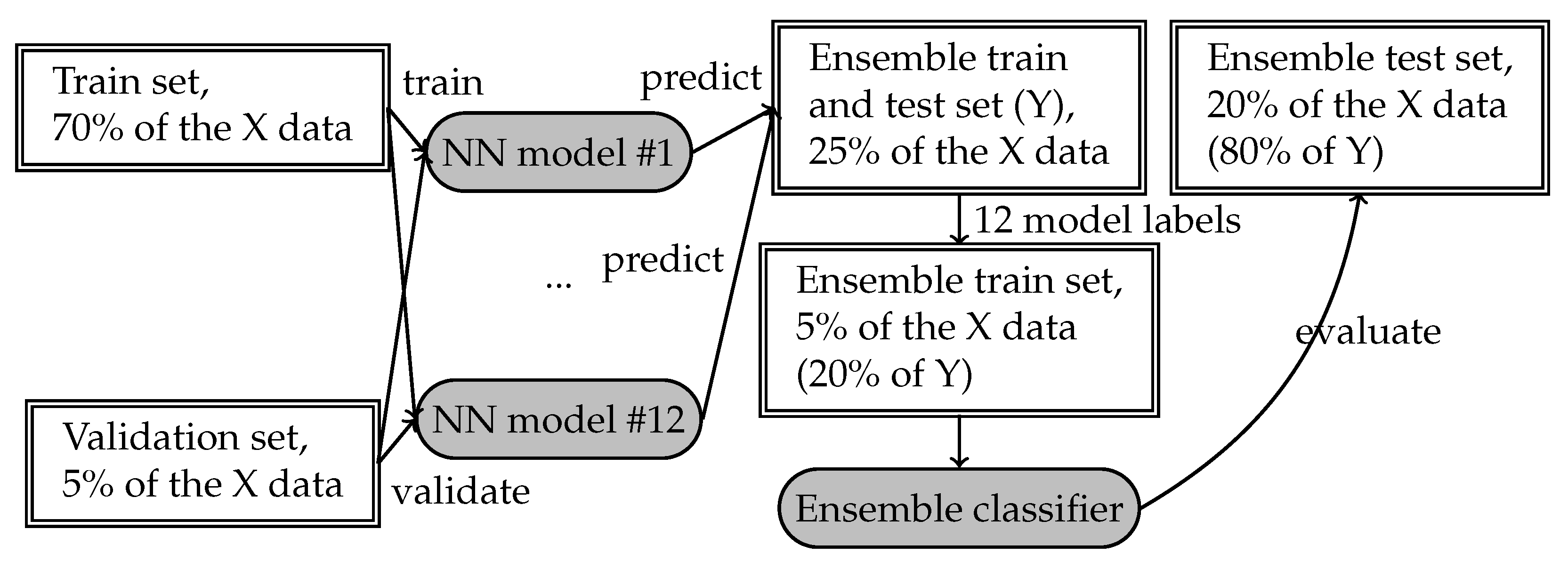
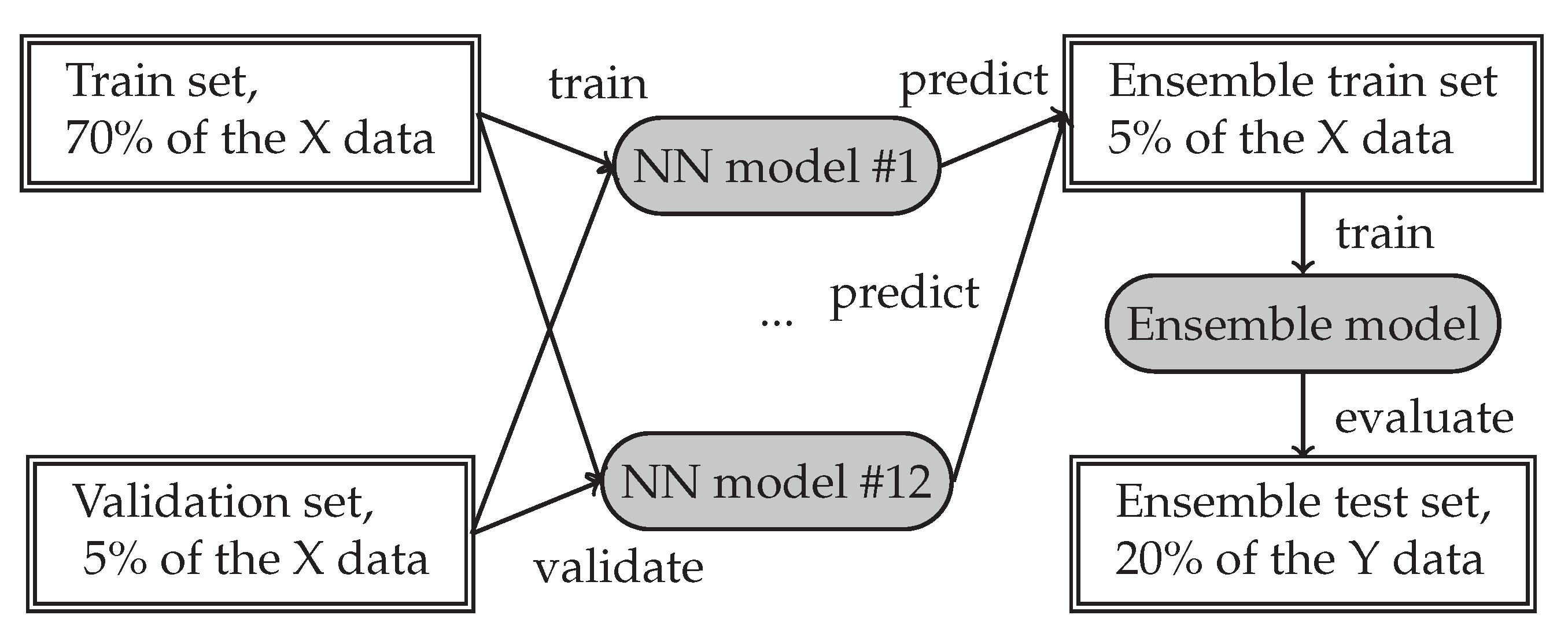
For the ensemble evaluation, we trained all 12 models and the ensemble classifier using the same pipeline as in
Section 3.3 on the training set (denoted as Dataset X in
Figure 7). Then, these 12 models produce the labels for both 5% of the Dataset X (20% from its test set that is used for training ensemble weights) and 20% of the Dataset Y (its entire test set). The ensemble model is trained on 5% of the Dataset X and applied on 20% of the Dataset Y, using labels produced by 12 trained individual models.
To make this process fully compatible to an in-domain testing procedure (depicted in
Figure 4 and
Figure 5), we used the same dataset splits both for evaluation of individual models (see
Figure 6) and for evaluation of ensemble models (see
Figure 7).
As we can see from
Table 6, all cases where the training set comes from one domain and the test set is from another domain produce the significantly lower accuracy than that reported in
Table 2,
Table 3,
Table 4 and
Table 5. This is a testament to the fact that general definition domain and mathematical domain are quite different.
4.9. Parameter Selection and Evaluation
Our work aimed to evaluate the effect of syntactic information for the task of definition extraction. The prior work [
20] in this field has demonstrated that relying on the word information alone (such as word embedding) does not produce good results. Furthermore, classification accuracy depends heavily on the dataset—higher accuracy scores are achieved on the WCL dataset [
32] by methods in [
20] and [
1] because both the word embeddings used for the task and the data originate in Wikipedia. On other datasets such as DEFT, W00, and our WFMALL accuracy scores of individual models (see
Table 2,
Table 3,
Table 4 and
Table 5) are significantly lower.
To combat this situation, we experimented with different neural models and their parameters, such as the number of layers, type of layers, learning rate, and so on. However, the classification accuracy was only slightly affected by the change in these parameters—for instance, increasing the number of training epochs above 15 did not improve the scores at all. The final parameters we used for our neural models appear in
Table 7.
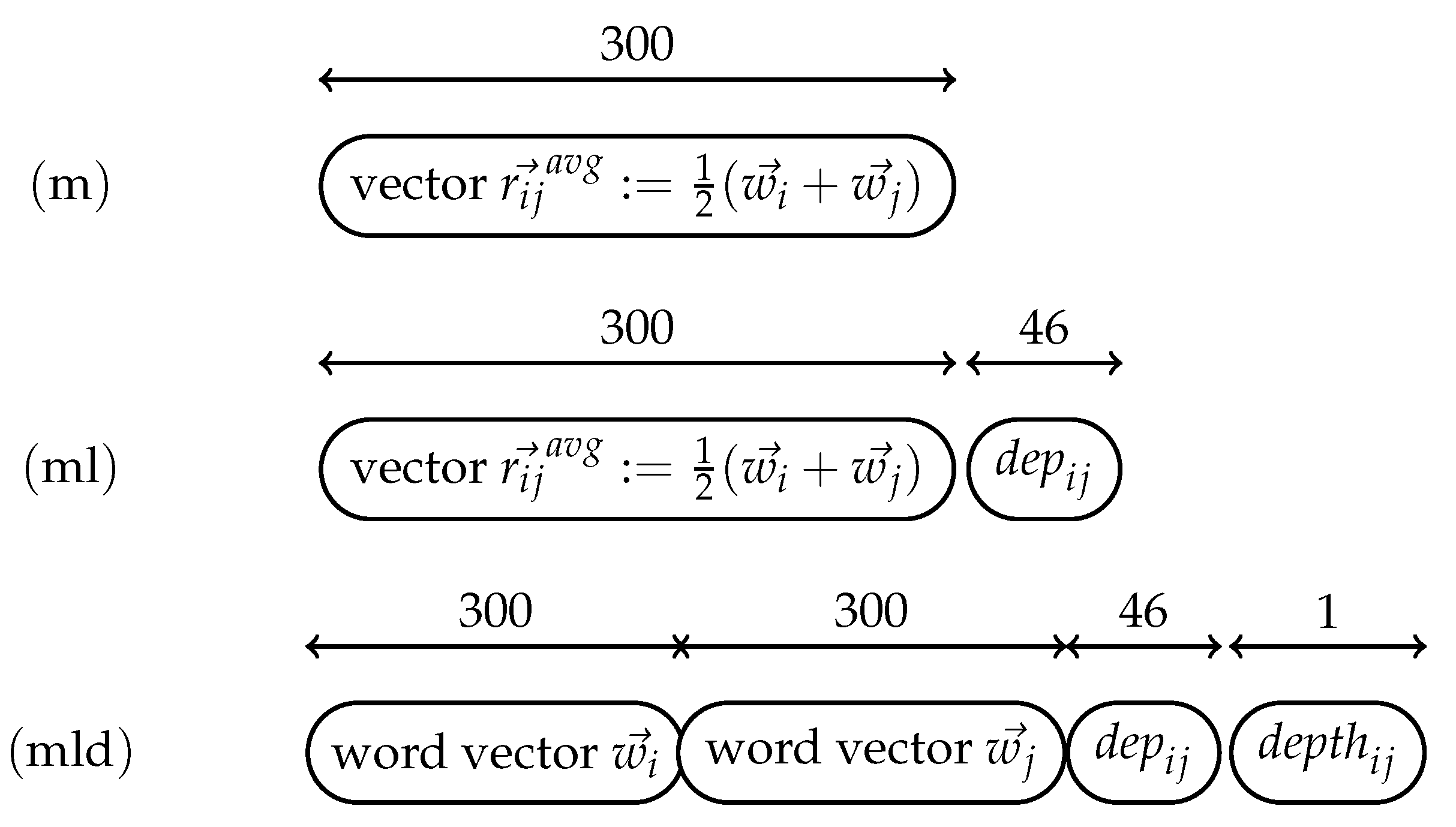
Furthermore, we incorporated syntactic information into our models using input representations depicted in
Figure 1. However, we observed that individual models rank differently on different datasets, and there is no clear advantage in using one specific syntactic representation because such a selection does not translate well across datasets. Therefore, we decided to use the ensemble model to compensate for variation in the data, and to use resampling to balance the data.
To analyze the importance and necessity of composition models in our ensemble, we performed feature selection by evaluating the information gain of labels produced by each model. The results are shown in
Table 8 for the four datasets; the highest ranking attributes are shown in bold. As can be seen, with one exception per dataset, all models with the first or only CNN layer are ranked higher than other models. As such, we can conclude that models that use CNN as their first layer are more successful and have higher influence on the ensemble scores, but their exact influence also depends on a dataset. However, feature backward elimination showed that all 12 models are necessary and produce the best accuracy in ensemble. Eliminating individual models one by one from the ensemble produced less accurate ensemble models.
4.10. Error Analysis
We tried to understand which sentences represented difficult cases for our models. During annotation process, we found that multiple sentences were assigned different labels by different annotators. Finally, the label for such sentences was decided by majority voting, but all annotators agreed that the decision was not unambiguous. Based on our observation and manual analysis, we believe that most of the false positive and false negative cases were created by such sentences. We categorized these sentences to the following cases:
Sentences describing properties of a mathematical object. Example (annotated (gold standard label = “definition”) as
definition):
An extremum may be local ( a.k.a. a relative extremum); an extremum in a given region which is not the overall maximum or minimum ) or global.
We did not instruct our annotators regarding labeling this sentence type and let them make decisions based on their knowledge and intuition. As result, this sentence type received different labels from different annotators.
Sentences providing alternative naming of a known (and previously defined) mathematical object. Example (annotated as
non-definition):
Exponential growth is common in physical processes such as population growth in the absence of predators or resource restrictions (where a slightly more general form is known as the law of growth).
We received the same decisions and the same outcomes in our dataset with this sentence type as with type (1).
Formulations—sentences that define some mathematical object by a formula (in contrast to a verbal definition, that explains the object’s meaning). Example (annotated as
non-definition):
lFormulas expressing trigonometric functions of an angle 2x in terms of functions of an angle x, sin(2x) = [FORMULA].
If both definition and formulation sentences for the same object were provided, our annotators usually assigned them different labels. However, rarely a mathematical object can be only defined by a formula. Additionally, sometimes it can be defined by both, but the verbal definition is not provided in an analyzed article. In such cases, annotators assigned the “definition” label to the formulation sentence.
Sentences that are parts of a multi-sentence definition. Example (annotated as
non-definition):
This polyhedron is known as the dual, or reciprocal.
We instructed our annotators not to assign “definition” label to sentences that do not contain comprehensive information about a defined object. However, some sentences were still annotated as “definition”, especially when they appear in a sequence.
Descriptions—sentences that describe mathematical objects but do not define them unequivocally. Example (annotated as
non-definition):
A dragon curve is a recursive non-intersecting curve whose name derives from its resemblance to a certain mythical creature.
Although this sentence resembles a legitimate definition (grammatically), it was labeled as non-definition because its claim does not hold in both directions (not every recursive non-intersecting curve is a dragon curve). Because none of our annotators was expert in all mathematical domains, it was difficult for them to assign the correct label in all similar cases.
As result of subjective annotation (which occurs frequently in all IR-related areas), none of the ML models trained on our training data were very precise with the ambiguous cases such as those described above. Below are several examples of sentences misclassified as definitions (false positives (with gold standard label “non-definition” but classified as “definition”)), from each type described in the list above:
Most misclassified definitions (false negatives) can be described by an atypical grammatical structure. Examples of such sentences can be seen below:
Once one countable set S is given, any other set which can be putinto a one-to-one correspondence with S is also countable.
The word cissoid means “ivy-shaped”.
A bijective map between two metric spaces that preserves distances,
i.e., d(f(x), f(y)) = d(x, y), where f is the map and d(a, b) is the distance function.
We propose to deal with some of the identified error sources as follows. Partial definitions can probably be discarded by applying part-of-speech tagging and pronouns detection. Coreference resolution (CR) can be used for identification of the referred mathematical entity in a text. Additionally, the partial definitions problem should be resolved by reduction of the DE task to multi-sentence DE. Formulations and notations can probably be discarded by measuring the ratio between mathematical symbolism and regular text in a sentence. Sentences providing alternative naming for mathematical objects can be discarded if we are able to detect the truth definition and then select it from multiple candidates. It can also be probably resolved with the help of such types of CR as split antecedents and coreferring noun phrases.
4.11. Discussion
As can be seen from all four experiments, ensemble outperforms individual models, despite latter being trained on more data. This outcome definitely supports the superiority of the ensemble approach for both domains.
It is worth noting that BERT did not perform well on our task. We explain it by the difference between the general domain of its training and our application domain of definitions and the lack of syntactic information in its input representation.
The scores of individual models approve again that syntactic information embedded into a sentence representation usually delivers better performance in both domains.
As our cross-domain evaluation results show, general definition domain and mathematical domain are quite different and, therefore, transfer cross-domain learning performs significantly worse than traditional single-domain learning.


