Unsustainability Risk of Bid Bonds in Public Tenders

Abstract

Public works contracts are commonly priced and awarded through a tender process. Each bidder joining the tender must underwrite a bid bond that guarantees their fitness as contractors in case of a win. The winning contractor also needs to underwrite a performance bond before entering the contract to protect the procuring entity against the performance risk arising during the execution phase. This study addresses the case when sureties refuse to issue the performance bond, despite having issued a bid bond to the same subject. A creditworthiness variation of the contractor during the tender or an excessive discount of the contract’s price may lead to this outcome. In that case, all the subjects involved are damaged. The surety who issued the bid bond has to indemnify the procuring entity. The contract award is nullified, which is financially harmful to both the contractor and the procuring entity. We show that sureties adopting a forward-looking risk appetite framework may prevent the demand for unsustainable performance bonds instead of addressing it by rejecting the bidders’ requests. The Solvency II regulatory framework, the Italian bidding law, and actual historical data available from the Italian construction sector are considered to specify a simplified model. The probability of unsustainable tender outcomes is numerically estimated by the model, together with the mitigating impact of a surety’s proper strategy.

1. Introduction

Sustainability is a complex and evolving concept that may include, inter alia, economic and financial considerations, environmental and social impacts, as well as political and legal aspects [1]. In public works, sustainability must be considered in its broadest meaning since all the aspects are relevant to the public entity that requires the execution of a project and the citizens who benefit from its fulfillment. However, also in this context, economic sustainability remains necessary to enable all the other possible forms of sustainability. Unfair pricing of the project implies a waste of public resources (when too high) or may result in a poor or even missed execution (when too low). Both cases have a negative impact, at least from a social perspective, but possibly also environmentally, depending on the specific situation.

Typically, the cost of a public construction project is determined by a tender promoted by the procuring entity. Nowadays, each country disciplines bid mechanisms underlying public tenders by a complex regulatory framework that guarantees fairness among participants and financial protection to the procuring entities. The leading economies share the main features of respective public bid laws (see, e.g., [2,3,4,5]). In particular, a system of guarantees is usually mandatory and involves insurance companies and financial institutions as sureties [6,7,8]. Each participant to a public tender must underwrite a bid bond to take part in the tender. The bid bond guarantees that the contract winner will satisfy all the requirements needed to become the contractor, including acquiring a performance bond. The values of the contract and the related performance bond are subjected to stochastic variations during the bidding process due to the tender rules. Hence, when the bid bond is issued, the surety has to consider the riskiness of the guaranteed participant concerning these variations and the sustainability of issuing a subsequent performance bond in case the bidder wins the contract.

There is a negative dependency between the final value of the contract and the notional value of the performance bond. This is because the public procuring entity wants to be protected against the performance risk of the winning contractor. Intuitively, the lower the final performance cost is, the higher the probability of poor performance or other breaches of contract is. Thus, the need for financial protection of the public entity increases accordingly. The final notional value of the performance bond may be too high for the risk appetite of the surety who has issued the bid bond of the winning bidder, significantly if the bidder’s creditworthiness has worsened during the tender process. If no other surety is available to issue the performance bond, the bid bond generates a claim. The surety who has issued it has to indemnify the procuring entity on behalf of the contractor, who cannot be awarded the contract.

During the last two decades, the increasing need for developing and improving public infrastructures in many countries has renewed the research interest on various financial, economic, and legal topics related to the construction industry. In particular, the attention to risk management tools and techniques in public works and large private projects has considerably increased, leading to an intense research activity [9,10,11,12]. In this context, surety bonds have been investigated mainly empirically, with particular reference to performance bonds and the benefits they produce in terms of risk mitigation. In these years, performance bonds have also been investigated with regards to their legal sustainability, depending on the specific regulatory framework of a considered country [13,14,15]. For example, in countries where these instruments have been introduced recently, it is worth considering the moral hazard of beneficiaries who abuse their right to call on the surety guarantees. The relevance of the problem has been assessed, and possible improvements to specific national laws are presented in [13,14]. Surety bonds have been investigated from an actuarial perspective as well, addressing both the problems of pricing them and measuring their mitigation effect on the underlying performance risk [16,17]. Results obtained in [16] imply that surety companies can help to mitigate the problem of contractors going bankrupt by their ability to perform a preliminary screening. Further, in [17] it is shown that contractors with a better standing are more likely to win the tender if sureties apply a risk-adjusted price to the performance bond. However, to date, the literature has focused only on investigating the performance risk and the likelihood that the winning contractor defaults during the execution of the public works.

This work investigates the case that the tender process may lead to an unsustainable outcome (i.e., the performance bond is not issued, and the tender process has to be reopened). This is relevant since the inefficiency of the tender process implies costs for all the subjects involved: the bidders, the sureties, and the public entity. Italian bid law [18,19] is considered to specify the tender mechanisms (e.g., the functional form that links the contract pricing and the notional value of the performance bond). A risk appetite framework is proposed to model the behavior of the sureties who support the bidders based on the Solvency II regulatory framework [20,21,22]. To the best of our knowledge, this is the first study that addresses this specific topic.

The work is organized as follows. Section 2 introduces the business and legal context of the investigated problem. The main features of the suretyship insurance business are reported, with a focus on the bid bond and the performance bond insurance products. Further, the Italian bidding law for public works is described. Section 3 models the sustainability of the tender outcome both for the bidders and the sureties. The Solvency II Standard Formula elements needed to design the surety’s risk appetite framework are introduced, and the bidder’s behavior is modeled considering their appetite for a minimum profit. Section 4 addresses the investigated problem. After introducing the distributional assumptions needed, we measure the probability of inefficient outcomes of public tenders through numerical simulations. The main results are summarized in Section 5.

2. Elements of Suretyship Insurance and the Italian Public Tenders

Suretyship policies provide a guarantee of performance and principles of various objectives and duties. They are commonly required to secure the obligations of the principal debtor (generally known as the principal) against the beneficiary. In the Solvency II framework, suretyship insurance is classified in Solvency II Line of Business 9 (also known as S2LoB 9), together with credit insurance. However, unlike in credit insurance, the suretyship insurer (also known as the surety) has a direct relation with the source of risk. The principal usually underwrites a surety policy because this is a requirement to engage the beneficiary in business.

Risks underlying surety policies can be very diverse from each other, ranging from performance risk in an engineering contract to moral hazard/operational risks in claiming a VAT credit to be refunded. Surety bonds fall under two categories [6]:

• Contract bonds, intended to guarantee the performance of contractual obligations, mainly in the areas of public works and private construction projects;
• Commercial bonds, intended to secure the performance of legal or regulatory obligations.

Without claim to completeness, examples of products belonging to each category are listed in

Table 1. A brief description of the main suretyship products.

Contract Bonds
Bid bond	Guarantees that a contractor has submitted a bid in good faith and intends to enter the contract in case of award
Performance bond	Offers protection from the case that a contractor fails to fulfill the terms of the contract
Advance payment bond	Guarantees that the contractor will be able to repay the procuring entity any funds received in advance
Payment bond	Protects the credit of workers, subcontractors, and suppliers against the contractor
Maintenance bond	Guarantees against defective workmanship or materials
Commercial Bonds
Customs bond	Assures customs authorities that an importer will pay the import duties required
Tax bond	Ensures the proper declaration and timely payment of taxes
License/permit bond	Guarantees the obligor’s compliance with laws
Court/fidelity bond	Guarantees the performance of fiduciaries’ duties and their compliance with court orders

.

This work is focused on two typical products in suretyship insurance among the ones listed above: the bid bond and the performance bond. The life cycle of these two products—depicted in Figure 1 and Figure 2—can be summarized as follows.

A procuring entity requires a generic “performance”, such as constructing infrastructures or supplying specific goods or services. Hence, the entity mentioned above uses a bidding process to select the best contractor for the assignment. Each contractor interested in submitting the bid has to underwrite a bid bond that guarantees the procuring entity against the case that the awarded contractor is not able to take charge of the required performance. Indeed, the contractor could go bankrupt during the bidding process, or some requirement necessary to fulfill the obligation could not be met (e.g., legal authorizations needed to perform the underlying task). In this case, the bidding process has to be reopened, and the insurer indemnifies the procuring entity.

In case the winning contractor satisfies all the requirements, a performance bond is still needed to close the bidding process. It is worth noticing that the insurer who has issued the bid bond may refuse to underwrite the performance bond. However, suppose the contractor cannot find another insurer available to underwrite the required performance bond. In that case, the tender is reopened, and thus the bid bond issuer has to indemnify the procuring entity. This mechanism implies that insurers who issue a bid bond share the subsequent performance risk with the procuring entity to some extent.

The phase after the bidding process is the execution phase when the obligation has to be fulfilled by the winner of the tender. The performance bond guarantees the beneficiary against the risk that the principal cannot satisfy the obligation’s timing or any other requirement. If the performance does not meet all the requirements declared in the bidding process, the insurer indemnifies the procuring entity.

Depending on the considered regulatory framework, the procuring entity can increase the duration or modify other features of the obligation during the execution phase. This is usually the case when the procuring entity is a public institution. When the risk underlying the performance bond is modified, the insurer may require the payment of a premium supplement but must accept to guarantee the beneficiary against the risk extension.

In the case of a claim, the subrogation phase takes place. Namely, the subrogation can be thought of as the set of rules that defines the insurer’s role when the execution phase is interrupted by a violation of the underlying obligation. Different regulatory frameworks define this concept in different ways.

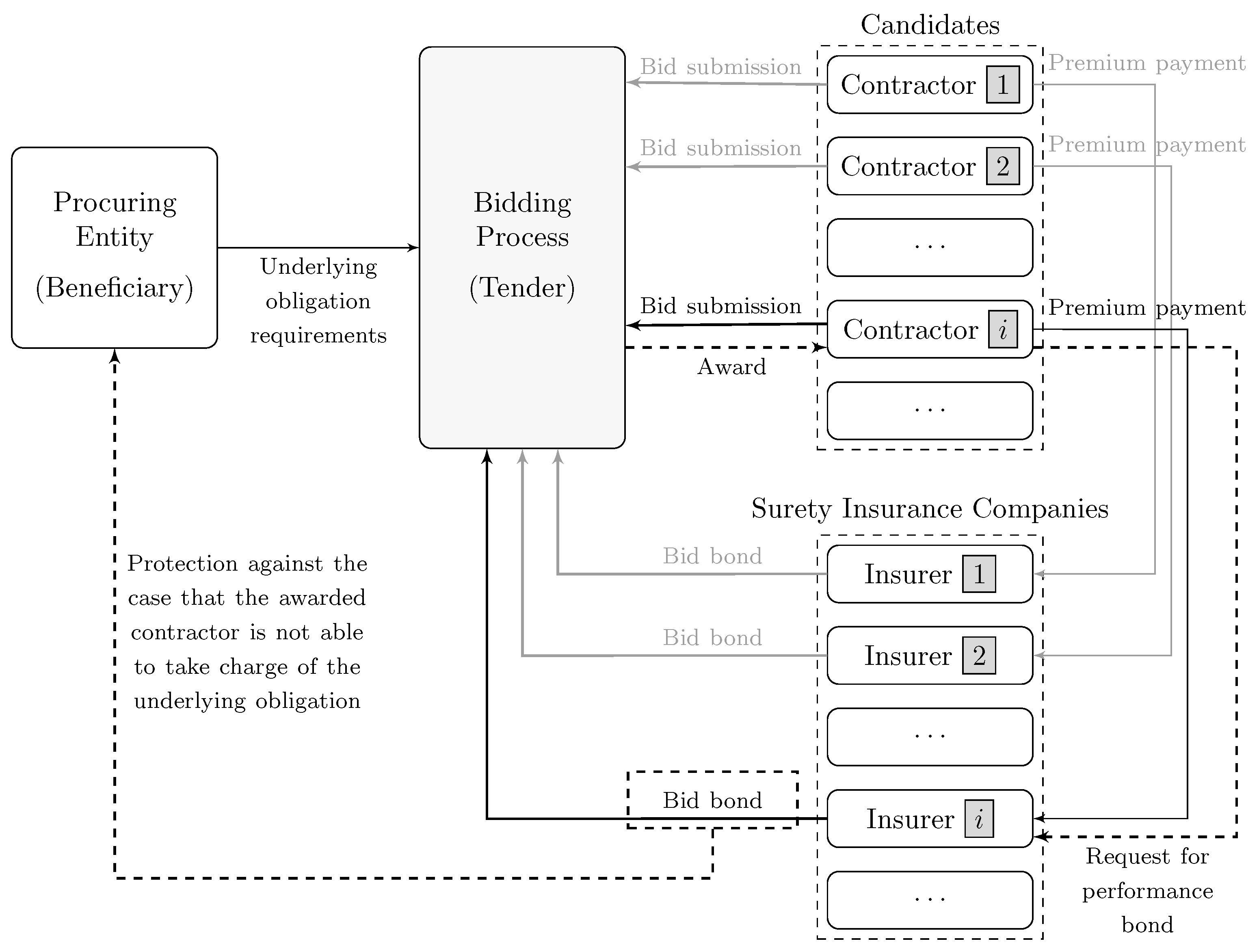
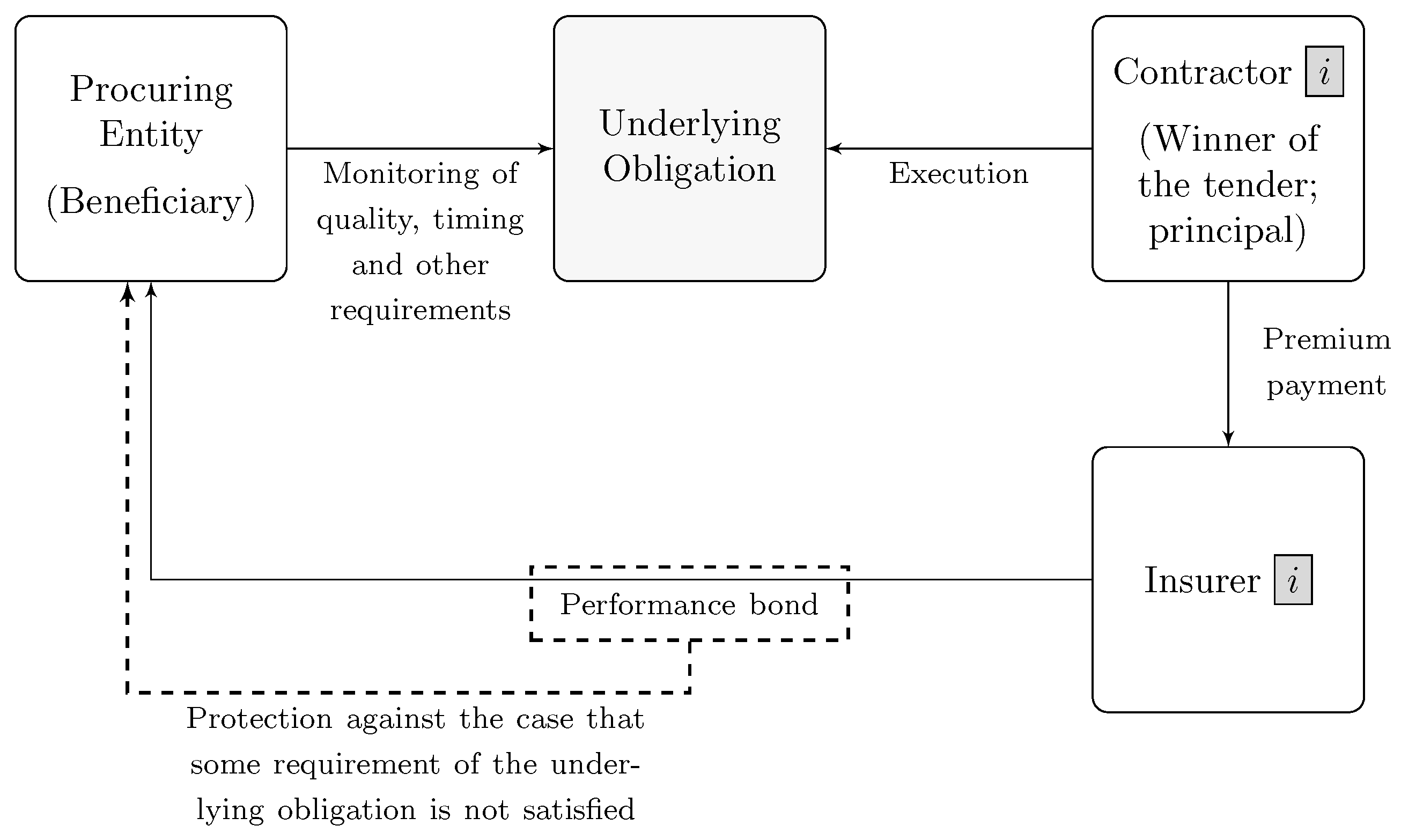
Bid and Performance Bonds: The Italian Case

According to the Italian bidding law [18], the exposure (in this study, “exposure” refers to the maximum claim size that a considered insurance contract covers without considering any recoverable) $N_B$ generated by a bid bond is typically fixed to a ${\alpha }_B=2\%$ fraction of the underlying obligation notional value $V_0$, established by the procuring entity at the beginning $t=t_0$ of the bidding process. However, depending on the risk profile of the obligation, the procuring entity may choose a different ${\alpha }_B$ value in the interval $[1\%,4\%]$.

The performance bond exposure $N_P$ likewise is represented as a fraction ${\alpha }_P$ of the obligation notional values $V_1$, re-estabilished at the time $t=t_1$ when the tender ends. Since each candidate contractor offers to take charge of the obligation at a cost that is lower than the auction base $V_0$, it holds $V_1<V_0$ by construction. However, the Italian law forbids to choose ${\alpha }_P$ and provides a mechanism to protect the beneficiary from the risk arising when $V_1\ll V_0$ (i.e., quality requirements of the obligation are likely to not be met). In fact, it holds

$${\alpha }_P\left(d_{01}\right)=a_P+max\{0;1-a_P-d_{01}\}+max\{0;1-2a_P-d_{01}\}$$

(1)

where $a_P=10\%$ and $d_{01}:=V_1/V_0$. Namely, the base value of ${\alpha }_P$ is equal to $10\%$, but it is increased by $1\%$ per each percentage point exceeding a $10\%$ bidding discount and by $2\%$ per each percentage point exceeding a $20\%$ bidding discount.

Hence, in the case of $V_1\simeq V_0$, ${\alpha }_B=2\%$ and ${\alpha }_P=10\%$, the exposure at risk guaranteed by a given performance bond is approximately five times the exposure at risk covered by the corresponding bid bond. However, depending on the choice of ${\alpha }_B$ and the value of $d_{01}$, the notional value $N_P$ of the performance bond can easily reach an amount ranging between 10 and 20 times the corresponding bid bond exposure $N_B$. This fact incentivizes the insurer to assess the contractor as accurately as possible when underwriting the bid bond to avoid the choice between the bid bond payment and the issue of a performance bond that causes the exposure generated by the contractor to be too big for the contractor’s worthiness.

The performance bond exposure decreases over time as the completion percentage of execution increases. The effective exposure can decrease up to $20\%$ of the initial exposure in $t=t_1$. However, the insurer is usually unaware of the execution status: there is no obligation for the beneficiary or the principal to keep the insurer updated unless a claim is notified.

In case of a claim, the insurer indemnifies the beneficiary, and then the subrogation takes place: the insurer acquires the right to recover from the principal the amount indemnified to the beneficiary [19].

3. Sustainability of a Bid Bond

In this section, the risk-adjusted economic sustainability of a bid bond is investigated. Section 3.1 presents the bidder’s perspective, while the risk appetite of the surety is discussed in Section 3.2. The procuring entity is protected by the mechanism described in Section 2, which rules the whole bidding process. In particular, Equation (1) fixes the notional value of the performance bond to cope with the performance risk of the winning bid. However, the tender process is sustainable for the procuring entity only if it leads to a sustainable outcome for both the contractor and the surety, such that the tender does not have to reopen. Hence, the sustainability conditions of all the subjects involved in the tender process are discussed in the following sections, explicitly or not.

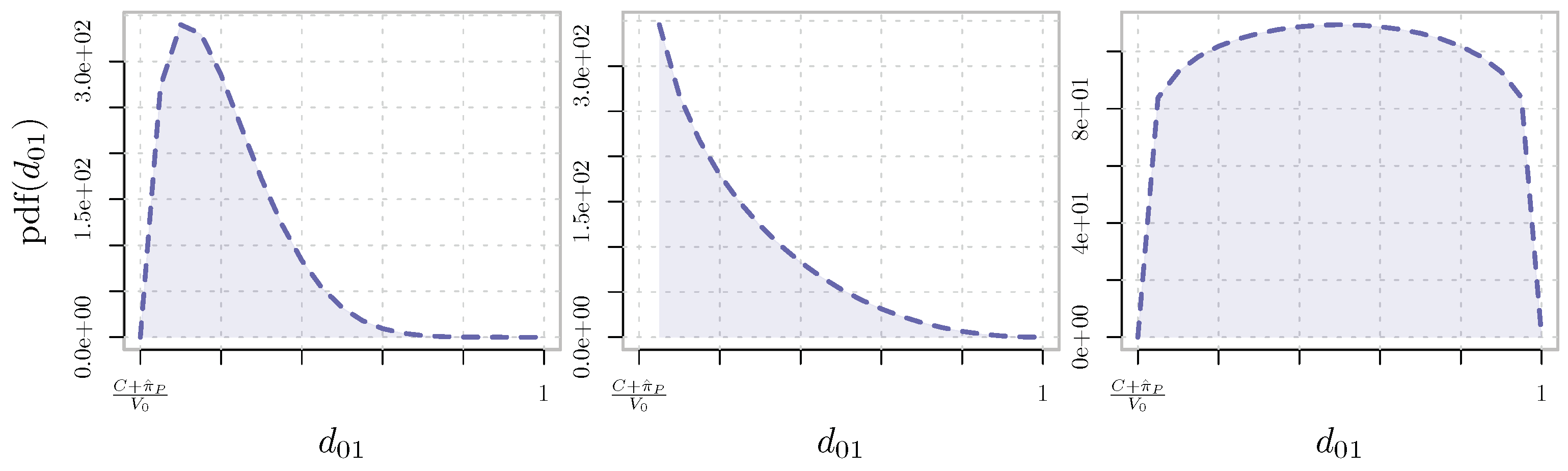
3.1. The Bidder’s Perspective

Let us assume that C is the contractor’s cost to fulfill the principal obligation (e.g., the construction of public infrastructures). Inflation effects on the price of raw materials are negligible through the period $(t_0,t_1]$ when the tender takes place. Further, all the bidders are supposed to have access to the same liquid market to get the needed workforce, materials, and instruments. Thus, C is supposed to be equal to all the competitors and independent from time. We can safely assume that C also includes a minimum target profit required by each contractor’s stakeholders. Its value remains (approximately) the same for all the bidders, even considering this additional contribution.

From a bidder’s perspective, $V_1$ has both natural upper and lower bounds. The upper bound ${\overline{V}}_1:=V_0>V_1$ holds true by construction, while the lower bound

$${\underline{V}}_1:=C+{\pi }_P\le V_1$$

(2)

is the amount needed by the bidder to cover the expected costs, the target profit, and the risk-adjusted price ${\pi }_P\left(d_{01}\right)$ of the performance bond. Filtered at $t_1$, the surety is assumed to price the performance bond according to a typical non-life actuarial pricing form [23,24] that accounts for expected losses, costs, and a prudential loading needed to compensate the surety’s risk aversion, the latter also being the surety’s profit. Hence, the price ${\pi }_P$ obeys the equation

$${\pi }_P=p_{12}{L}_P{N}_P+(r+s){\pi }_P,$$

(3)

where $p_{12}$ is the breach/default probability of the contractor over the execution period, $(t_1,t_2]$ and thus, $p_{12}{L}_P{N}_P$ is the expected loss contribution. Indeed, $L_P\in (0,1]$ is the loss given default mitigation coefficient. It considers both the expected recovery of the surety from the contractor after the claim and the possible reduction of $N_P$ at the claim time due to the partial fulfillment of the guaranteed obligation. The term $r{\pi }_P$ is the compensation for the risk aversion of the surety’s stakeholders, where r scales as the cost-of-capital rate. The contract’s price ${\pi }_P$ is approximately proportional to the contract’s contribution to the solvency capital requirement (SCR) needed by the insurer to guarantee its solvency in the Solvency II Standard Formula framework. Moreover, the surety’s costs are assumed to be proportional to ${\pi }_P$ and are taken into account by the cost ratio s term. The discount contribution of non-zero risk-free interest rates is neglected. As discussed in Section 2, it holds

$$N_P={\alpha }_P\left(d_{01}\right)V_1,$$

(4)

where also $V_1=d_{01}{V}_0$ is dependent on $d_{01}$. Hence, the risk-adjusted price of the performance bond is

$${\pi }_P\left(d_{01}\right)=\frac{p_{12}{L}_P}{1-r-s}{\alpha }_P\left(d_{01}\right)d_{01}{V}_0$$

(5)

The price ${\pi }_B$ of the bid bond follows the same structure and assumptions (see Remark 2 below).

Equations (2) and (5) imply that the public tender is sustainable for the winner of the tender, only if the inequality

$$[1-\frac{p_{12}{L}_P}{1-r-s}{\alpha }_P\left(d_{01}\right)]d_{01}\ge \frac{C}{V_0}$$

(6)

is verified. It is worth noticing that $d_{01}$ is deterministic in the bidder’s perpective, since it is a bidder’s decision. On the other hand, $p_{12}$ and r are unknown to the bidder, but a non-binding offer from the surety market is usually available on request, allowing the bidder to consider the provisional price

$${\widehat{\pi }}_P=\frac{{\widehat{p}}_{12}{L}_P}{1-r-s}{N}_P\left({\widehat{d}}_{01}\right)$$

(7)

where ${\widehat{p}}_{12}$ is the bidder’s probability of default in $(t_1,t_2]$ estimated by the surety conditioned to the information available in $t_0$, and ${\widehat{d}}_{01}$ represents the expected value of $d_{01}$ under the same filtration ${\mathcal{F}}_{t_0}$. Hence, the boundaries ${\overline{V}}_1$ and ${\underline{V}}_1$ imply the determination of a compact interval where the contractor’s choice of $d_{01}$ in $t_0$ is rational.

$$\frac{C+{\widehat{\pi }}_P}{V_0}\le d_{01}\le 1$$

(8)

Condition (8) confirms two intuitive facts. First, the least risky bidder can afford to offer the greatest decrease of the starting price $V_0$, implying that the better the creditworthiness is, the higher the probability of winning the tender is. Second, the lower the ratio $C/V_0$ is, the smaller the minimum sustainable $d_{01}$ value is.

Remark 1.

LHS of inequality (8) is a special case of inequality (6), conditioned to the information available in $t_0$. Even if each bidder behaves rationally, placing a bid $d_{01}\left(t_0\right)$ in the interval defined in condition (8), in $t_1$ it is still possible that the winner of the tender is awarded with a non-sustainable contract, because satisfying (8) in $t_0$ does not imply that (6) will be fulfilled in $t_1$. This uncertainty motivates the existence of prudential bids that are greater than the minimum rational level $\frac{C+{\widehat{\pi }}_P}{V_0}$.

Remark 2.

The cost ${\pi }_B$ of the bid bond is negligible in the framework introduced above. In fact, it holds ${\pi }_B\ll {\pi }_P$, because ${\alpha }_B\ll {\alpha }_P$ (see Section 2) and $t_1-t_0\ll t_2-t_1$. Further, the bid bond generates a claim only if the insured bidder defaults and is the winner of the tender. Hence, assuming to know the number N of participants involved in the tender process and considering approximately equal probabilities of being awarded among participants, the price of the bid bond can be written as

$${\pi }_B=\frac{1}{N}\frac{p_{01}{L}_B}{1-r-s}{\alpha }_B{V}_0.$$

(9)

under the same assumptions considered for ${\pi }_P$ in Equation (5). As discussed above, the probabilities of winning are not uniform among the bidders, but such precise information is not available to a surety that guarantees just one of them in most cases. In general, considering the respective durations of bid bonds and performance bonds, and the $1/N$ factor as well, it holds

$$\frac{1}{N}{p}_{01}\ll p_{12},$$

(10)

that strengthens the validity of ${\pi }_B\ll {\pi }_P$.

The bid bond prices should be regarded more as “generic” expenses of the contractor than costs related to specific tenders, given that each contractor has to allocate a share of economic resources to participate in tenders, to win a part of them at most.

3.2. The Surety’s Perspective

The subject who acts as the surety may be either a bank or an insurance company operating in the suretyship insurance line of business. We consider the latter case in the following, assuming that the Solvency II framework regulates the surety. This assumption copes with the investigated problem (i.e., the sustainability of bid bonds in Italy—a country where Solvency II is applied to the insurance market).

According to the Solvency II Directive [20] (Article 44), each insurer must define a set of rules, known as Risk Appetite Framework (also RAF), which aims to limit the capital absorption level below a given fraction of the own funds. This concept is then implemented in the Italian insurance law as well [25]. Since the RAF should discipline the business strategy and the management actions, the problem of the efficient capital allocation among the insurer’s lines of business has been widely investigated in the actuarial literature (see, e.g., [26,27] and references therein).

However, this work focuses on the sustainability of a specific suretyship contract. Hence, our interest in a surety’s RAF is limited to the subset of rules that may limit the surety’s risk appetite against Premium Risk and the related Catastrophe Man-Made Risk in the Solvency II Standard Formula framework. On the other hand, the maximum acceptable amount of capital absorbed by the suretyship line of business is assumed to be fixed. Let us consider a (sub)portfolio composed of suretyship policies only. According to the Solvency II Standard Formula [21,22], such a portfolio exposes the insurer to three risk components of the Underwriting Risk:

i.

The Premium Risk, whose Solvency Capital Requirement (SCR) is measured as

$$\begin{array}{cc}\hfill {\mathrm{SCR}}_{\mathrm{Pr}}& :=3{\sigma }_{\mathrm{Pr}}{V}_{\mathrm{Pr}},\hfill \\ \hfill V_{\mathrm{Pr}}& :=max\{P_{\mathrm{Next}};P_{\mathrm{Last}}\}+F{P}_{\mathrm{Existing}}+F{P}_{\mathrm{Future}};\hfill \end{array}$$

(11)

where $P_{\mathrm{Last}}$ and $P_{\mathrm{Next}}$ are the premiums earned in the last 12 months and the premiums to be earned in the next 12 months, respectively; $F{P}_{\mathrm{Existing}}$ and $F{P}_{\mathrm{Future}}$ are the expected present value of the premiums to be earned after the following 12 months for existing contracts and for contracts whose initial recognition date falls in the following 12 months (for future contracts, premiums earned during the first 12 months after the initial recognition date are excluded from $F{P}_{\mathrm{Future}}$ contribution to volume measure), respectively; and ${\sigma }_{\mathrm{Pr}}=19\%$ is the coefficient of variation associated to this sub-module of risk by the European regulator. The geographical diversification factor is not considered in Equation (11), since we are considering risks arising from Italian contractors only. The effect of reinsurance is ignored as well for this risk component and the next two listed below.

ii.

The Catastrophe Recession Risk, whose Solvency Capital Requirement (SCR) is measured as

$${\mathrm{SCR}}_{\mathrm{Rec}}:=P_{\mathrm{Next}}$$

(12)

iii.

The Catastrophe Default Risk, whose Solvency Capital Requirement (SCR) is measured as

$${\mathrm{SCR}}_{\mathrm{Def}}:=\mathrm{lgd}(L{E}_1+L{E}_2)$$

(13)

where $L{E}_i$ ($i=1,2$) are the first and the second largest exposures in the considered portfolio and $\mathrm{lgd}=10\%$ is a loss given default coefficient fixed by the European regulator.

The Standard Formula aggregation rule for the risk components listed above is

$$\begin{array}{ccc}\hfill {\mathrm{SCR}}_{\mathrm{Udw}}& =& {\left({\mathrm{SCR}}_{\mathrm{Pr}}^2+2\rho {\mathrm{SCR}}_{\mathrm{Pr}}{\mathrm{SCR}}_{\mathrm{Cat}}+{\mathrm{SCR}}_{\mathrm{Cat}}^2\right)}^{\frac{1}{2}},\hfill \\ \hfill {\mathrm{SCR}}_{\mathrm{Cat}}& =& {\left({\mathrm{SCR}}_{\mathrm{Def}}^2+{\mathrm{SCR}}_{\mathrm{Rec}}^2\right)}^{\frac{1}{2}},\hfill \end{array}$$

(14)

where $\rho =25\%$ and ${\mathrm{SCR}}_{\mathrm{Udw}}$ is the Underwriting Risk measure under the assumption that all the risk components different from $i.-iii.$ are null, as futher specified in the following remark.

Remark 3.

Equation (14) measures only a part of the SCR_Udw that each suretyship insurance company has necessarily to cover. In particular, the Reserve Risk sub-module has been ignored, since this study is focused on the growth of Premium Risk due to newly underwritten contracts, which is directly related to the sustainability of the new policies.

This simplification can be interpreted either as the assumption of instantaneous indemnifications (i.e., the surety opens and immediately closes the reserve provision associated with each claim, keeping the Reserve Risk negligible) or as the assumption that the surety’s RAF disciplines the Reserve Risk capital requirement separately from the Premium and Catastrophe risks. Indeed, the latter assumption is more likely than the first one.

Lapse Risk is ignored since it is not considered relevant to this line of business.

Loosely speaking, in this context, the risk measure ${\mathrm{SCR}}_{\mathrm{Udw}}$ scales approximately with the size of the future earned premiums that, according to Equations (5) and (9), are proportional to the notional exposures ($N_B={\alpha }_B{V}_0$ or $N_P={\alpha }_P{V}_1$ in case of bid bonds or performance bonds, respectively) of each bond underwritten and to the corresponding claim probabilities ($\frac{1}{N}{p}_{01}$ or $p_{02}$ respectively). Further, both $N_B$ and $N_P$ are proportional to the initial value $V_0$ of the contract and the performance bond exposure $N_P$ has also a non-linear positive dependence on $d_{01}$, as shown in Equations (1) and (4).

For the sake of simplicity, let us consider a stable or expanding business, so that

$$max\{P_{\mathrm{Next}};P_{\mathrm{Last}}\}=P_{\mathrm{Next}}.$$

(15)

The simplification introduced in Equation (15) implies that Equation (14) can be rewritten as follows

$${\mathrm{SCR}}_{\mathrm{Udw}}=\sqrt{9{\sigma }_{\mathrm{Pr}}^2{(P+F)}^2+6\rho {\sigma }_{\mathrm{Pr}}(P+F)\sqrt{D^2+P^2}+D^2+P^2}$$

(16)

where we use the compact notation $D:={\mathrm{SCR}}_{\mathrm{Def}}$ and $P:=P_{\mathrm{Next}}$. Equation (16) allows to estimate the marginal contribution $\delta {\mathrm{SCR}}_{\mathrm{Udw}}$ to the capital requirement originated by a newly underwritten policy

$$\begin{array}{ccc}\hfill \delta {\mathrm{SCR}}_{\mathrm{Udw}}(P,F,D)& =& {\mathrm{SCR}}_{\mathrm{Udw}}(P+\delta P,F+\delta F,D)-{\mathrm{SCR}}_{\mathrm{Udw}}(P,F,D)\hfill \\ \hfill & =& C_P\delta P+C_F\delta F+\cdots ,\hfill \end{array}$$

(17)

where

$$\begin{array}{}\mathrm{(18)}& \hfill C_P& :=& \frac{1}{{\mathrm{SCR}}_{\mathrm{Udw}}(P,F,D)}\left[9{\sigma }_{\mathrm{Pr}}^2(P+F)+3\rho {\sigma }_{\mathrm{Pr}}\frac{D^2+P^2+P(P+F)}{\sqrt{D^2+P^2}}+P\right],\hfill \mathrm{(19)}& \hfill C_F& :=& \frac{1}{{\mathrm{SCR}}_{\mathrm{Udw}}(P,F,D)}\left[9{\sigma }_{\mathrm{Pr}}^2(P+F)+3\rho {\sigma }_{\mathrm{Pr}}\sqrt{D^2+P^2}\right],\hfill \end{array}$$

$\delta P$ is the new policy’s contribution to $P_{\mathrm{Next}}$, and $\delta F$ is the new policy’s contribution to $F{P}_{\mathrm{Existing}}+F{P}_{\mathrm{Future}}$. D is assumed to be constant, which is generally true, unless the new policy’s exposure exceeds $L{E}_2$ in Equation (13).

The premium accrual is linear in time, although the risk generated by the policy decreases as a non-linear function of the time-to-maturity. Hence, it holds that

$$\begin{array}{ccc}\hfill \delta P& =& \pi \frac{min\{T-t,1\}}{T-t_0},\hfill \\ \hfill \delta F& =& \pi \frac{max\{T-t-1,0\}}{T-t_0},\hfill \end{array}$$

(20)

where $\pi$ is the bond premium, t is the observation date, and $t_0$ and T are the recognition date and the maturity date of the bond, respectively. Abrupt variations of ${\mathrm{SCR}}_{\mathrm{Udw}}$ may occur in case an insured bidder wins a tender and the surety issues the performance bond as needed. In this case, the bid bond premium ${\pi }_B$ is replaced by the corresponding performance bond premium ${\pi }_P\gg {\pi }_B$ (see Remark 2). The surety’s RAF should aim to prevent the exposure from “jumping”, associated with the conversions of bid bonds into performance bonds, which may lead to a breach of the established ${\mathrm{SCR}}_{\mathrm{Udw}}$ threshold level.

Many policy underwriters are simultaneously and independently operating on behalf of the surety. Hence, the contribution of each issued bond to ${\mathrm{SCR}}_{\mathrm{Udw}}$ cannot be taken into account instantaneously. In a realistic situation, ${\mathrm{SCR}}_{\mathrm{Udw}}$ is likely to be updated quarterly or twice a year, while new policies are issued daily or weekly. Hence, the surety may choose to maintain ${\mathrm{SCR}}_{\mathrm{Udw}}$ at a safe distance from a threshold ${\overline{\mathrm{SCR}}}_{\mathrm{Udw}}$ by defining a maximum acceptable $\delta {\mathrm{SCR}}_{\mathrm{Udw}}$ caused by each newly underwritten policy. Equations (5), (9), (17), and (20) imply that the maximum acceptable exposure ${\overline{E}}_p$ of a new policy scales as $p^{-1}$, where p is the claim probability of the policy. Namely, it holds

$${\overline{E}}_p=\frac{{\overline{\delta \mathrm{SCR}}}_{\mathrm{Udw}}}{C_P\frac{min\{T-t,1\}}{T-t_0}+C_F\frac{max\{T-t-1,0\}}{T-t_0}}\frac{1-r-s}{L}{p}^{-1},$$

(21)

where ${\overline{\delta \mathrm{SCR}}}_{\mathrm{Udw}}$ is the maximum acceptable variation of ${\mathrm{SCR}}_{\mathrm{Udw}}$ due to the new risk. $C_P$ and $F_P$ depend on the last updated values of ${\mathit{SCR}}_{\mathrm{Udw}}$, P, F, and D. Terms beyond the first order in Equation (17) are assumed to be negligible.

Two concerns should be addressed before using Equation (21) to define a (simplified) surety RAF. First, if the contract is a bid bond, the case the contractor wins the tender and, thus, a performance bond is needed and must be considered. This issue is addressed later in Definition 2. Further, sureties want to limit their concentration of exposure against each contractor. Thus, a penalty term due to existing exposures that the same contractor generates should be considered.

To address the latter issue, the threshold ${\overline{\delta \mathrm{SCR}}}_{\mathrm{Udw}}$ is lowered by the first-order contribution to $SC{R}_{\mathrm{Udw}}$ of the policies already underwritten by the same contractor. Applying Equation (17) once again, we have the new threshold

$${\overline{\delta \mathrm{SCR}}}_i:=max\left\{0,{\overline{\delta \mathrm{SCR}}}_{\mathrm{Udw}}-C_P\sum _{j\in {\left\{i\right\}}_t}\delta P_{ij}-C_F\sum _{j\in {\left\{i\right\}}_t}\delta F_{ij}\right\}$$

(22)

where ${\left\{i\right\}}_t$ is the sub-portfolio of policies existing in t and underwritten before t by the i-th contractor, and

$$\begin{array}{ccc}\hfill \delta P_{ij}& =& {\pi }_{ij}\frac{min\{T^{\left(ij\right)}-t,1\}}{T^{\left(ij\right)}-t_0^{\left(ij\right)}},\hfill \\ \hfill \delta F_{ij}& =& {\pi }_{ij}\frac{max\{T^{\left(ij\right)}-t-1,0\}}{T^{\left(ij\right)}-t_0^{\left(ij\right)}}\hfill \end{array}$$

(23)

are the contributions to P and F of the j-th policy in $\left\{i\right\}$, given the same notation used in Equation (20). It is worth noticing that the new threshold can be equal to zero, in case the concentration level on the i-th contractor has already exceeded the surety’s risk appetite.

To handle the first concern on Equation (21), the surety’s RAF can be defined as follows.

Definition 1

(Backward-looking Surety’s RAF). The RAF is specified by the function $\Psi :(0,1)\to {\mathbb{R}}_{+}$, defined as follows. $\Psi \left(p_{iJ}\right)$ is the maximum increment of exposure ${\overline{\delta E}}_i$ that the surety is allowed to guarantee against the i-th risky contractor (${|\left\{i\right\}}_t|=J-1$), by issuing the new $iJ$-th bond whose claim probability is equal to $p_{iJ}$. $\Psi :p_{iJ}\mapsto {\overline{\delta E}}_i$ has the form

$$\Psi \left(p_{iJ}\right)=\frac{{\overline{\delta \mathrm{SCR}}}_i}{C_P\frac{min\{T^{\left(iJ\right)}-t,1\}}{T^{\left(iJ\right)}-t_0^{\left(iJ\right)}}+C_F\frac{max\{T^{\left(iJ\right)}-t-1,0\}}{T^{\left(iJ\right)}-t_0^{\left(iJ\right)}}}\frac{1-r-s}{L}{p}_{iJ}^{-1}.$$

(24)

Thus, the surety refuses to underwrite each J-th contract, such that ${\delta E}_{iJ}>\Psi \left(p_{iJ}\right)$.

The RAF in Definition 1 is backward-looking in the sense that the acceptance or rejection of a given contract depends only on the contribution of the contract to the last SCR measured. As anticipated, Definition 1 does not offer solution to the first issued raised above (i.e., bid bonds which cope with Definition 1 may lead to performance bonds that exceed the frontier defined in Equation (24) in the future). Definition 2 also handles this issue.

Definition 2

(Forward-looking Surety’s RAF). The RAF is specified by the couple $\{\Psi (·);p_{\Psi }\}$. The function $\Psi :(0,1)\to {\mathbb{R}}_{+}$ defines the maximum increment of exposure ${\overline{\delta E}}_i$ that the surety is allowed to guarantee against the i-th risky contractor (${|\left\{i\right\}}_t|=J-1$) by issuing the new $iJ$-th bond whose claim probability is equal to $p_{iJ}$. $\Psi :p_{iJ}\mapsto {\overline{\delta E}}_i$ has the form stated in Equation (24). The tolerance $p_{\Psi }\in (0,1)$ is the maximum admissible probability that a risk underwritten in t implies a breach of the boundary $\{p_{i^{\prime }{j}^{\prime }},{\overline{\delta E}}_{i^{\prime }}\}$ at some $t^{\prime }>t$ for all $i^{\prime },j^{\prime }$. Namely, the $iJ$-th bond can be underwritten in t only if

$$\mathbb{P}\left[\left.\Psi \left(p_{i^{\prime }{j}^{\prime }}\left(t^{\prime }\right)\right)<E_{i^{\prime }}\left(t^{\prime }\right)\right|{\mathcal{F}}_t\right]<p_{\Psi }\forall t^{\prime }>t,i^{\prime },j^{\prime }\in \mathbb{N},$$

(25)

where $\mathbb{P}$ is real-world probability measure available to the surety. A bond that satisfies both conditions (24) and (25) by t is sustainable in the surety’s perspective.

The Solvency II Standard Formula is based on some simplifying assumptions that also affect Equation (24).

First, premiums as a volume measure establish a link between the riskiness of each risk source (i.e., the contractor in this case) and the capital requirement. However, in case the premium rate is fixed at the issuing date $t_0$, it is related to the contractor’s standing at $t_0$, but it may not be representative of the contractor’s riskiness when $SC{R}_{\mathrm{Udw}}$ is evaluated.

Further, the fraction of premium to be earned by the surety decreases linearly over time. Hence, the negative dependence between risk and residual time-to-maturity is taken into account. However, the non-linear decreasing of risk by time—as shown, e.g., in Equation (7)—is replaced by a linear dependency.

Despite these limitations, the Standard Formula represents a breakeven point between simplicity and effectiveness. Being an established standard in the European insurance industry, it is worth considering it when defining the RAF used to investigate the sustainability of a given bid bond. Internal model approaches are possible as well and are not affected by the limitations mentioned above. However, in this work, we are interested in investigating possible paradoxes arising in a standard context. Hence, we chose to use the Standard Formula exclusively.

Definition 1 introduces a maximum exposure-at-risk ${\overline{E}}_i$ per contractor, implicitly. The value of ${\overline{E}}_i$ depends on the standing of the i-th contractor and the remaining time-to-maturity of each underwritten contract, in agreement with intuition. On the other hand, Definition 2 also forbids less trivial cases.

A bid bond that satisfies condition (24) in $t_0$ may still not comply with condition (25), in case it holds

$$\mathbb{P}\left[{\Psi }^{-1}\left(E_{iJ+1}\left(t_1\right)\right)<p_{iJ+1}\left(t_1\right)|{\mathcal{F}}_{t_0^{\left(iJ\right)}}\right]>p_{\Psi },$$

(26)

where the bid bond is the J-th policy underwritten with the i-th contractor and the subsequent performance bond (in case the contractor wins the tender) is the $J+1$ policy.

It is worth noticing that Equation (25) implies restrictions stronger than the one stated in Equation (26). Let us consider the $iJ$-th bid bond mentioned above, assuming that it satisfies condition (24) and does not have the problem in Equation (26). Even in such a case, the bond could still not satisfy condition (26) due to portfolio issues. In fact, when the number of simultaneously active bid bonds is large enough, the probability that one of them results in a future performance bond not compliant with condition (24) exceeds $p_{\Psi }$, even if the last underwritten bid bond complies with the RAF when considered stand-alone.

The “global” sustainability of a bid bond (i.e., in the context of the surety’s portfolio of underwritten bonds) is addressed in Section 4 numerically.

4. Measuring and Managing the Unsustainability Scenarios in Public Tenders

This section addresses the sustainability issues introduced in Section 3 by implementing the surety’s RAF proposed in Definitions 1 and 2. A model is introduced in Section 4.1 to simulate the tenders. Each simulation considers three alternate versions of the surety: without an RAF, adopting a backward-looking RAF as per Definition 1, and adopting a forward-looking RAF as per Definition 2. The results obtained by the Monte Carlo simulations are presented in Section 4.2, Section 4.3, and Section 4.4, respectively.

4.1. Simulation of Tenders from a Surety’s Perspective

In the following paragraphs, the model employed to simulate the tenders of public works is described. The model aims to highlight that unsustainable requests for a performance bond are possible when considering realistic dynamics of default (or breach) probabilities associated with each bidder. Further, the model is employed to investigate the effectiveness of the RAF strategies implemented by the surety.

A realistic model of the Italian public works market should include some aspects not considered in this section, such as the actual number of tenders per year where the considered surety guarantees at least a bidder and the distribution of the public works costs C. However, the data needed to calibrate such a model are non publicly available, and the model itself would not fit better for the purpose of this study than the toy model introduced here.

Let us consider a where the elementary time step $\delta t$ is a quarter long. We consider a surety with access to ${10}^3$ public tenders per quarter, issuing a bid bond to at least a participant per tender since there is no need to simulate tenders where the considered surety has no business. We assume that the initial price of each tender is a uniform r.v.

$$V_0\sim {\mathrm{Unif}}_{\left[C,150\%C\right]}.$$

(27)

Both the boundaries $min{V}_0$ and $max{V}_0$ are admitted to represent a possible misjudgment of the procuring entity. In fact, $V_0=C$ leaves no room to lower the initial price or to aim for an extra profit, implying that no bidder is joining the tender. Further, in case $V_0=150\%C$, Equation (1) implies that $E_P/E_B$ can reach a value of 45 and above, increasing the probability that the required performance bond violates Equation (24) and, thus, that sureties reject the (unsustainable) winner’s request for a performance bond.

Thus, it is natural to assume a positive dependency between $V_0/C$ and the number of potential bidders $\tilde{N}$ interested in joining the tender. We chose the form $\tilde{N}=⌊100\left(e^{V_0/C-1}-1\right)⌉$, which implies a realistic range $\tilde{N}\in \{0=N_{V_0=C},\cdots ,N_{V_0=1.5·C}=65\}$. However, the $N\le \tilde{N}$ constructors who actually join the tender are the ones able to make a bid according to the condition (8), depending on the values of ${\widehat{\pi }}_P$ and $V_0$.

The surety can issue more than a bid bond per tender (up to N), increasing the probability that one among its insured bidders wins the contract and is required to underwrite the corresponding performance bond. However, considering the competition in the surety market, we assume that the number of bidders n joining the same tender and insured by the same surety is distributed as a shifted Poisson r.v. Namely, $\tilde{n}-1\sim \mathrm{Pois}\left({\lambda }_B\right)$, where ${\lambda }_B=0.1$ and $n=min\{\tilde{n};N\}$.

The parameter ${\alpha }_B$ is assumed to be distributed as a categorical r.v. with probability mass function

$$f\left({\alpha }_B\right)=\left\{\begin{array}{cc}0.2,\hfill & {\alpha }_B\in \{1\%;3\%;4\%\};\hfill \\ 0.4,\hfill & {\alpha }_B=2\%;\hfill \\ 0.0,\hfill & \mathrm{otherwise}.\hfill \end{array}\right.$$

(28)

where the mode is fixed at $2\%$, as anticipated in Section 2.

To estimate claim probabilities and their dynamics, we consider historical time series of performing (“PL”) and non-performing loans (“NPL”) [28], publicly available from the Bank of Italy [29]. This choice is justified by the assumption that the claim probability of a contractor is completely correlated to its creditworthiness. This is true in the extreme case of bankruptcy, which implies the contractor’s inability to be operating. In general, it is a fair approximation, although other elements of technical nature (e.g., unforeseen geological features of the building location) may contribute to the performance risk in specific cases.

Time series ${\mathrm{PL}}_t$ and ${\mathrm{NPL}}_t$ are quarterly available by ATECO 2007 economic sector (i.e., our data are restricted to the “constructors” sector), size of loan s (three clusters) and geographical location g of the Italian debtor (five clusters). Hence, dynamics of claim probability can be specified by considering 15 bivariate time series ${\{{\mathrm{PL}}_t;{\mathrm{NPL}}_t\}}_{sg}$, where ${\mathrm{PL}}_t$ is the number of performing loans at the first day of the t-th quarter, while ${\mathrm{NPL}}_t$ is the number of loans that become past due during the t-th quarter.

Since we need to represent a significant number of contractors by introducing a parsimonious number of parameters, we choose to apply the CreditRisk${}^{+}$ model [30,31] to describe the dependence structure among the claims and the marginal volatility of each cluster probability of default. The CreditRisk${}^{+}$ model defines the dependence among defaults (or other absorbing events, such as breaches of contracts) through an array of latent market factors $\mathbf{\Gamma }\in {\mathbb{R}}_{+}^K$, where ${\Gamma }_k\sim \mathrm{Gamma}({\sigma }_k^{-2},{\sigma }_k^2)$, ($k=1,\cdots ,K$). It holds that $\mathbf{E}\left[{\Gamma }_k\right]=1$ and $\mathrm{Var}\left[{\Gamma }_k\right]={\sigma }_k^2$ by construction. The market factors alter the parameter’s value of the r.v. $Y_i(t,t^{\prime })$, which represents the occurence of a claim generated by the i-th contractors in the time interval $(t,t^{\prime }]$. In its original formulation, the model [30] is defined in a single-time-scale framework and $Y_i\dot{\sim }\mathrm{Pois}\left(p_i\right)$, where

$$p_i(\mathbf{\Gamma }):=q_i·\left({\omega }_{i0}+\sum _{k=1}^K{\omega }_{ik}{\Gamma }_k\right)$$

(29)

and the factor loadings ${\omega }_{ik}$ are supposed to be all non-negative and to sum up to unity:

$$\begin{array}{cc}{\omega }_{ik}\ge 0,\hfill & i=1,\cdots ,N,k=0,\cdots ,K,\hfill \\ {\displaystyle \sum _{k=0}^K{\omega }_{ik}=1,}\hfill & i=1,\cdots ,N.\hfill \end{array}$$

(30)

We consider the model’s generalization recently proposed in [32], which has also been applied to credit and suretyship insurance [33]. The advantage of this choice is the possibility to calibrate the model by using the quarterly time series available and using it to estimate both the bid bond claim probabilities $p_{01}(t,h\left(i\right))$ and the corresponding performance bond claim probabilities $p_{12}(t,h\left(i\right))$, where $h=1,\cdots ,15$ labels the cluster of the i-th bidder.

We assume that each bid bond has a 3-month coverage period on the interval $(t=t_0,t_1=t+\delta t]$, while each performance bond has a 5-year coverage period on the interval $(t_1,t_1+20\delta t]$. This simplification is a part of the toy framework that we are defining since the duration of public works depends on each project’s features and size. However, it is numerically sound since a tender process takes a few months to close, while a public works project typically lasts a few years. Hence, a two-time-scales parameterization is needed to price both the bid and the performance bond.

According to [32], the claim event in CreditRisk${}^{+}$ framework can be modeled as $Y_i(t,t^{\prime })\sim \mathrm{Bernoulli}\left(p_i(t,t^{\prime })\right)$, where the parameter $p_i$ has an exponential dependency on the latent factors. Namely, under our set of assumptions, it holds that

$$\begin{array}{}\hfill \mathrm{(31)}& \hfill p_{01}(t_0,h)& =& 1-exp\left[-q_h\left({\omega }_{h0}+\sum _{k=1}^K{\omega }_{hk}{\Gamma }_k\left(t_0\right)\right)\right],\hfill \mathrm{(32)}& \hfill p_{12}(t_1,h)& =& 1-exp\left[-20q_h\left({\omega }_{h0}+\frac{1}{20}\sum _{\tau =0}^{19}\sum _{k=1}^K{\omega }_{hk}{\Gamma }_k(t_1+\tau \delta t)\right)\right],\hfill \end{array}$$

where $\tau \in \mathbb{N}$ is the index used to label each quarter. Further, assuming that the surety has developed an internal rating model such that reliable estimates of

$$\left\{\mathbf{\Gamma }\left(t\right):t=t_0,\cdots ,t_0+19\delta t\right\}|{\mathcal{F}}_{t_0},$$

we can represent the possible fluctuations in performance bond pricing by considering ${\widehat{p}}_{12}=p_{12}\left(t_0,h\left(i\right)\right)=p_{12}\left(t_1-\delta t,h\left(i\right)\right)$, while the (correct) estimate $p_{12}$, which allows the computation of ${\pi }_P$, shall not be available until $t=t_1$.

Let us consider the time series ${\{{\mathrm{PL}}_t;{\mathrm{NPL}}_t\}}_{sg}$ available in [29], from the first quarter of 2016 to the first quarter of 2021, to calibrate the CreditRisk${}^{+}$ model. The generalized covariance estimator defined in [32], the decomposition technique introduced in [34], and the standard regularization technique described in [35] return the result in

Table 2. The complete set of parameters $\widehat{\mathsf{\Omega }},{\widehat{\sigma }}_{\Gamma }^2$ necessary to specify the dependence structure in CreditRisk${}^{+}$ model applied to the Italian “Constructors” economic sector.

s	g	h	${\mathit{q}}_{\mathit{h}}$	$\mathit{k}=$	0	1	2	3	4	5
1	North-West	1	0.0050	${\omega }_{hk}=\left\{\begin{array}{}\\ \\ \\ \\ \\ \\ \\ \\ \\ \\ \\ \\ \\ \\ \\ \\ \\ \\ \\ \end{array}\right.$	0.516	0.246	0.025	0	0.212	0
1	South	2	0.0095		0.473	0.220	0.019	0.216	0	0.072
1	Islands	3	0.0098		0.559	0.231	0	0.210	0	0
1	North-East	4	0.0040		0.658	0.254	0.088	0	0	0
1	Center	5	0.0079		0.026	0.234	0.070	0.432	0	0.238
2	North-West	6	0.0079		0.509	0.228	0	0.028	0.235	0
2	South	7	0.0137		0.651	0.292	0.057	0	0	0
2	Islands	8	0.0158		0.455	0.266	0	0.036	0.237	0.005
2	North-East	9	0.0073		0.628	0.281	0.086	0.006	0	0
2	Center	10	0.0126		0.590	0.281	0.057	0.016	0	0.056
3	North-West	11	0.0130		0.091	0.235	0	0.134	0.443	0.096
3	South	12	0.0147		0.467	0.236	0.048	0	0.127	0.122
3	Islands	13	0.0185		0.619	0.333	0	0	0	0.049
3	North-East	14	0.0134		0.611	0.265	0.050	0	0.068	0.005
3	Center	15	0.0178		0.325	0.251	0.099	0	0	0.326
				${\sigma }_k^2=$		2.417	0.157	0.052	0.049	0.044

.

Remark 4.

Claims are not simulated in our setting, although the CreditRisk${}^{+}$ framework is explicitly designed to do it. In fact, they are not relevant to the part of the surety’s RAF addressed in this study. Occurred claims affect mainly the reserve provision and the Reserve Risk capital requirement. On the other hand, they may lead to a slight decrease of ${\mathit{SCR}}_{\mathit{Cat}}$ or ${\mathit{SCR}}_{\mathit{Pr}}$, since claims generated by suretyship insurance products are absorbing events. Each policy may generate one claim at most during the coverage period, implying the zeroing of both the corresponding exposure and future premiums (if any).

The framework is completed by associating each i-th bidder to its $h\left(i\right)$-th cluster. This is achieved by modeling the position of the public works underlying each tender as a categorical random variable. The probability associated with each g-th area ($g=1,\cdots ,5$) is proportional to the number of performing borrowers belonging to that area observed in the construction sector by the first quarter of 2021. This is equivalent to assuming a correspondence between demand and offer in this economic sector (i.e., the presence of many constructors implies a relevant number of public tenders and vice versa). Assuming that all the bidders belong to the same area where the public works must be executed, their distribution among the three loan classes is modeled in a similar way, considering a categorical variable per geographical area g, where probabilities are proportional to the number of performing borrowers observed in the cluster $sg$ ($s=1,2,3$), conditioned to g.

It is worth recalling that the public works tenders in Italy can be classified as first-price, sealed descending bid auctions (for complete classification of auctions and a deep theoretical discussion, see, e.g., [36,37]). The bid domain is compact, and the winner is the author of the lowest bid in a set of non-identically distributed bids. Hence, we cannot use the Fisher–Tippett–Gnedenko theorem [38,39], which is commonly applied to model the distribution of the winning bid in the ascending bid auctions (see, e.g., the recent paper [40], where a Weibull distribution is considered). Thus, we need to determine the winning bid numerically, considering that each rational bidder chooses its $d_{01}$ according to condition (8).

A non-uniform distribution is assumed over each i-th domain to take into account the appetite of each bidder for obtaining the contract. Namely, it holds that

$$\frac{d_{01}{V}_0-C-{\widehat{\pi }}_P\left(i\right)}{V_0-C-{\widehat{\pi }}_P\left(i\right)}\sim \mathrm{Beta}(\alpha ,\beta )$$

(33)

where multiple specifications have been tested for the parameters set $(\alpha ,\beta )$, as represented in Figure 3: $\mathrm{mode}\left[\mathrm{pdf}\left(d_{01}\right)\right]$ tends to $(C+{\widehat{\pi }}_P)/V_0$ at increasing bidder’s appetite for winning the tender, while it tends to $V_0$ at increasing appetite for profit. However, no relevant effect of the $(\alpha ,\beta )$ choice is observed on the results presented in Section 4.2, Section 4.3, Section 4.4 and Section 4.5. Hence, only the choice $(\alpha ,\beta )\equiv (1.80,7.20)$ is considered in Figure 4, Figure 5, Figure 6 and Figure 7.

The winner of each tender is the lowest simulated bid per tender/scenario. The bidders are indexed in simulations ($i=1,\cdots ,N$). In doing so, the case where the winning bidder is among the ones guaranteed by the considered surety is explicitly represented.

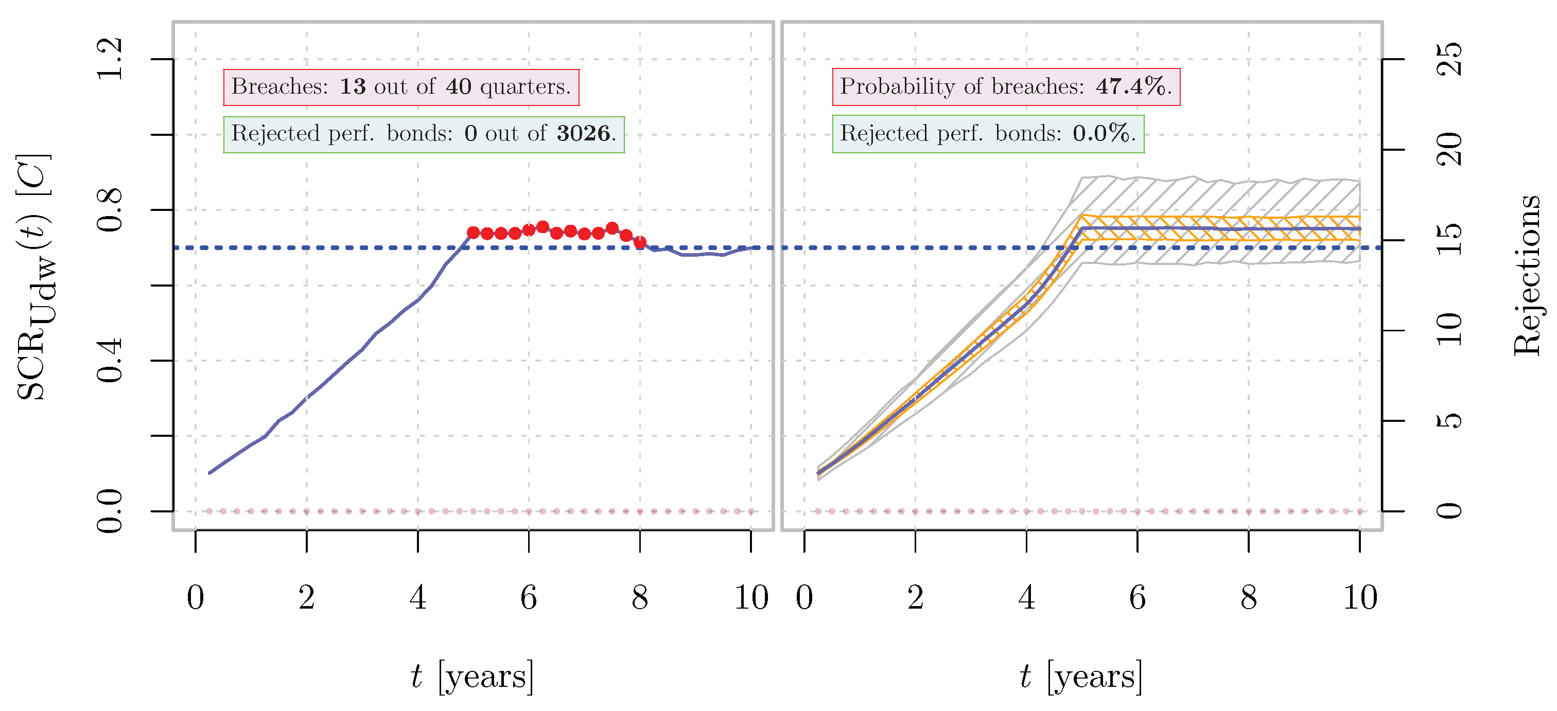
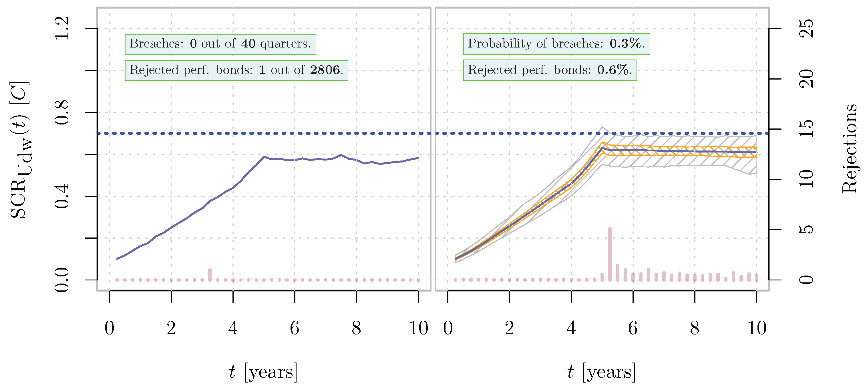
4.2. Dynamics of the Capital Requirement without Taking Management Actions

Let us consider a suretyship insurance company that operates as a surety in the framework introduced in Section 4.1. The surety is supposed to start operating in $t=0$. It is worth recalling that the duration of a bid bond is established to be equal to three months, while each performance bond is assumed to expire after five years. Thus, as expected, the surety ${\mathrm{SCR}}_{\mathrm{Udw}}$—as defined in Equation (16)—reaches an equilibrium after five years, considering a stable flow (on average) of new contracts per year (Figure 4).

Without loss of generality, we choose ${\overline{SCR}}_{\mathrm{Udw}}=0.7C$, which is below the equilibrium level ${\mathrm{SCR}}_{\mathrm{Udw}}(t>5)\approx 0.75C$ obtained numerically. The surety is supposed to increase its sales volume until its risk appetite level is reached. Then, a risk appetite framework is introduced to discipline the underwriting process, as discussed in Section 3.2. Hence, in a liquid market, a surety with a higher risk appetite or a larger amount of its own available funds than the one considered in our simulations would reach the same equilibrium state at a different ${\mathrm{SCR}}_{\mathrm{Udw}}$ level.

4.3. Dynamics of the Capital Requirement Adopting a Backward-Looking RAF

In Section 4.2, the surety has reached an equilibrium state that is slightly above its risk appetite level. Thus, an RAF is needed to prevent the occurrence of breaches ${\mathrm{SCR}}_{\mathrm{Udw}}\left(t\right)>{\overline{\mathrm{SCR}}}_{\mathrm{Udw}}$. The same simulations presented in Figure 4 are re-performed, applying the management actions implied by Definition 1, ceteris paribus.

The level ${\overline{\delta \mathrm{SCR}}}_{\mathrm{Udw}}$ is needed to specify $\Psi (·)$. It has to be as high as possible to refuse the minimum number of contracts per unit of time, conditioned to avoid breaches or, at least, make them improbable enough according to the surety’s risk appetite. In the example, we chose

$${\overline{\delta \mathrm{SCR}}}_{\mathrm{Udw}}\left(t\right)=max\left\{0;min\left\{{\overline{\mathrm{SCR}}}_{\mathrm{Udw}}-{\mathrm{SCR}}_{\mathrm{Udw}}(t-\delta t);\delta {\mathrm{SCR}}_{\mathrm{Udw}}\left[{\Phi }_{{\pi }_P}^{-1}\left(0.95\right)|{\mathcal{F}}_t\right]\right\}\right\}$$

where ${\Phi }_{{\pi }_P}(·)$ is the cumulative distribution function of the performance bond prices ${\pi }_P$ and $\delta {\mathrm{SCR}}_{\mathrm{Udw}}\left[·|{\mathcal{F}}_t\right]$ is the marginal contribution of a given contract underwritten in t to ${\mathrm{SCR}}_{\mathrm{Udw}}$. $\delta {\mathrm{SCR}}_{\mathrm{Udw}}$ is evaluated by applying the linear approximation stated in Equation (17).

Namely, when the last measure ${\mathrm{SCR}}_{\mathrm{Udw}}(t-\delta t)$ done until t is far enough from the threshold ${\overline{\mathrm{SCR}}}_{\mathrm{Udw}}$, we aim not to reject more than $5\%$ of the performance bond requested by the insured bidders who win their respective tenders. In case the distance ${\overline{\mathrm{SCR}}}_{\mathrm{Udw}}-{\mathrm{SCR}}_{\mathrm{Udw}}(t-\delta t)$ approaches zero or negative values, the RAF constraint becomes stronger up to blocking the acquisition of new contracts at all, until an acceptable ${\mathrm{SCR}}_{\mathrm{Udw}}$ level is restored. Figure 5 shows the effectiveness of this approach. Breaches are observable in tail scenarios, almost only in the region ($t\simeq 5$) where the SCR regime is changing from expansion to equilibrium. The small number of breaches and the RAF’s reaction implies a fraction of performance bonds rejected slightly above the $5\%$ target level.

4.4. Dynamics of the Capital Requirement Adopting a Forward-Looking RAF

As discussed above, the surety should avoid the rejection of a performance bond as much as possible. This case opens the possibility that the tender must be reopened if no other surety is willing to issue the performance bond instead of the surety that has issued the bid bond to the winning contractor. Further, in a market where sureties are comparable, the rejection of a request by a company implies that the other companies in the same market are likely to do the same, leading to a claim generated by the bid bond.

Hence, it is worth addressing this issue by implementing the forward-looking RAF introduced in Definition 2. It is not necessary to establish $p_{\Psi }$ explicitly. The probability that a performance bond generates a breach is an increasing function of $V_0/C$. Loosely speaking, a higher starting price implies that the winning bid—always close to C—corresponds to a greater discount $1-d_{01}$. Thus, a higher ${\alpha }_P$ can be expected as well, increasing the probability of a breach ${\overline{\delta \mathrm{SCR}}}_{\mathrm{Udw}}$.

Even without knowing the analytical form of the dependencies described above, the qualitative picture is enough to implement the constraint (25) as

$${\Phi }_{V_0/C}^{-1}\left(0.75\right)>{\left(\frac{V_0}{C}\right)}_k$$

(34)

where ${\Phi }_{V_0/C}(·)$ is the cumulative distribution function of $\frac{V_0}{C}$, and ${\left(\frac{V_0}{C}\right)}_k$ is the ratio observed in the k-th tender. The percentile $0.75$ has been chosen numerically with the aim of minimizing both the number of rejected performance bond requests and the frequency of SCR breaches. Bid bonds that do no cope with Equation (34) are rejected, preventing a possible unsustainable request for a performance bond (in case the bidder wins).

Given the additional constraint, we can weaken the other introduced in Section 4.3, passing from 0.95 to 0.99 (i.e., we aim to reject up to $1\%$ of performance bonds, to limit both the claims arising from the corresponding bid bonds and the surety’s reputational risk). Results are exposed in Figure 6, where the number of rejected performance bonds decreases.

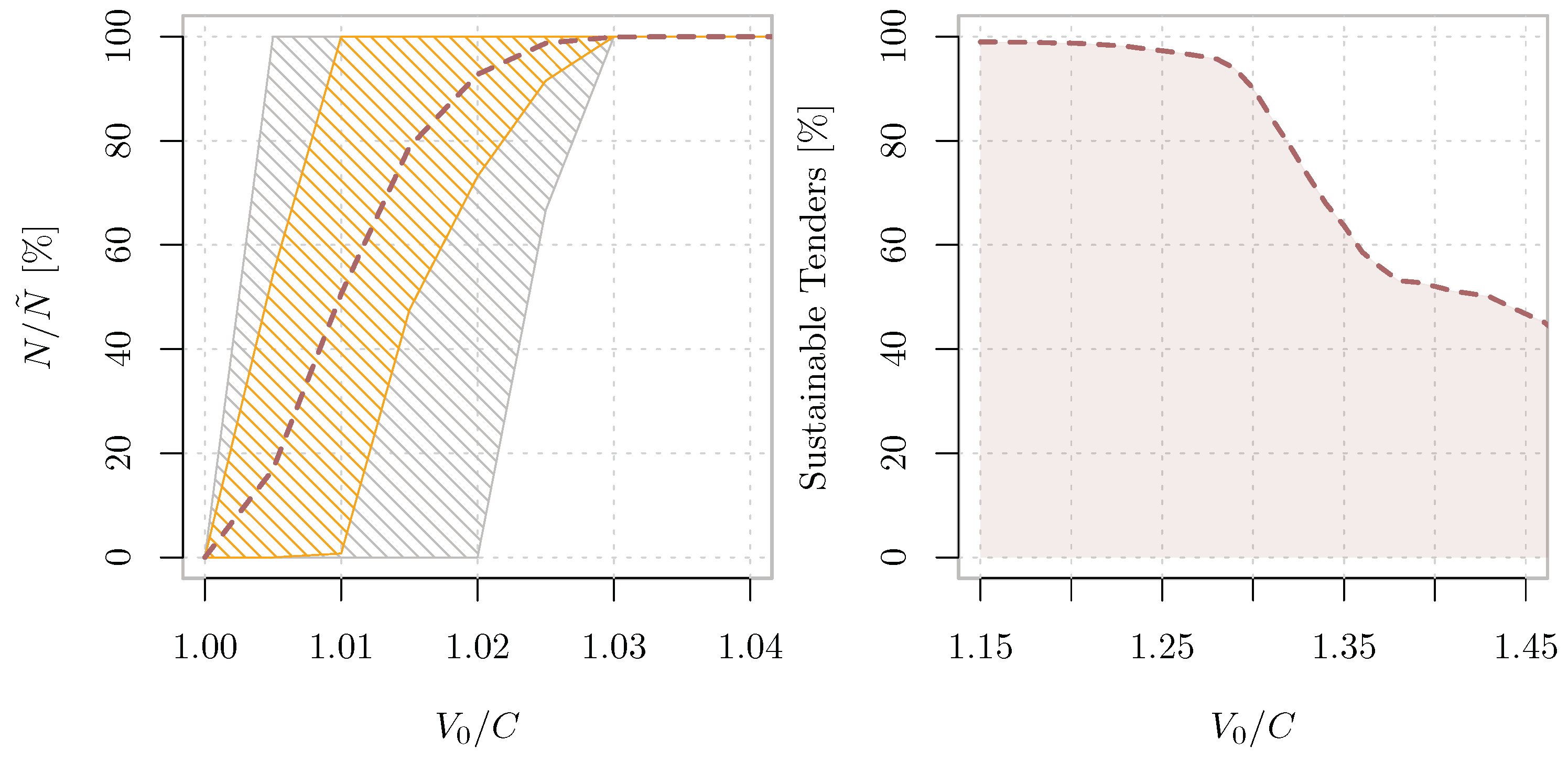
4.5. The Role of the Procuring Entity

As shown in Section 4.4, a surety that implements a forward-looking RAF can prevent the majority of unsustainable tender outcomes, avoiding rejecting performance bond requests from the winners and the possible subsequent need for reopening the tender.

However, unsustainability issues originate from a poor choice of starting price by the public procuring entity. The left panel of Figure 7 shows how a starting price near the breakeven level (i.e., $V_0\simeq C$) disincentivizes constructors to join the bid due to the constraints introduced in condition (8). It is worth noticing that this result is independent of the assumption made about the dependency $\tilde{N}\left(V_0\right)$. A tender that does not attract participants is clearly unsustainable from an economic perspective. The resources invested in promoting it are wasted, and the public works cannot be executed. Further, the opposite case (i.e., $V_0\gg C$) also implies the economic unsustainability of the tender, as the tender outcome implies $N_P/N_B\gg 1$ and thus an excessive risk for the surety (i.e., an unsustainable cost for the winning bidder or the inability to underwrite the mandatory performance bond). The right panel of Figure 7 shows the results of our simulations in this perspective: the fraction of requests for a performance bond rejected by a given surety increases from ≈0% to ≈50% as $V_0$ passes from ≈1.25 C to ≈1.45 C.

Remark 5.

Figure 7 shows that the tender is almost surely sustainable, depending on the procuring entity’s proper choice of the $V_0$ value. This fact implies that the case ${\pi }_P\gg {\widehat{\pi }}_P$, due to the worsening of a bidder’s creditworthiness during the tender process, has a negligible impact. The numerical evidence copes with the following intuition: since the tender lasts a few months, a relevant change in a bidder’s credit standing is unlikely during such a short period.

5. Conclusions

This study highlights the existence of an economic unsustainability risk for the tenders that award public works contracts. The Italian bidding law and the Solvency II regulatory framework are explicitly considered to model the behavior of the three subjects involved in the tender process: the procuring entities, the bidders, and the sureties. Numerical simulations show that this risk can be mitigated and prevented by the proper choices of both the surety and the procuring entity.

In Section 3, sustainability conditions are stated for both the bidders and the sureties. In particular, sureties can protect their SCR target levels by applying an RAF, as requested by the Solvency II Directive. In Section 3.2, we proposed two simplified RAFs, both based on the linearization of the Solvency II Standard Formula. The first one (i.e., “backward-looking”—Definition 1) aims only to protect the surety’s SCR level, regardless of the effects on the tender process. A boundary $(p;{\overline{E}}_p=K{p}^{-1})$ is shown to separate sustainable new exposures $E\le {\overline{E}}_p$ from the unsustainable ones ($E>{\overline{E}}_p$), depending on the default probability p associated to the considered contractor. A closed-form expression for K is provided from the Standard Formula prescription to evaluate the non-life underwriting risk module for the S2LoB 9-Credit & Suretyship Insurance. We show that the sureties can protect both themselves and the tender process by applying a “forward-looking” RAF, such as the one proposed in Definition 2. A numerical comparison among the two RAFs was presented in Section 4.3 and Section 4.4, showing that the latter can actually protect all the three subjects involved in the tender process.

While the surety can mitigate the unsustainability risk, the public procuring entity can prevent it by establishing an acceptable starting price for the tender. Our simulations suggest that $V_0/C\in [1.05,1.25]$ is the most sustainable choice in a realistic setting, where the Italian constructors’ default probability is modeled by applying the CreditRisk${}^{+}$ framework to recent historical data.

The proposed framework can be further investigated and improved in future studies. In particular, the Standard Formula approach can be replaced by a Partial Internal Model to define the two RAFs. The specific features of other regulatory frameworks diverse from the Italian bidding law may be investigated as well, provided that historical information to calibrate the model is publicly available for each considered country. Further, two limitations of this study are reported as follows, which can be addressed in further studies as well: First, both the procuring entity and the surety are assumed to perform error-free estimates. The procuring entity could actually choose $V_0$ poorly because of a bad strategy or the error affecting its C measure. The surety may perform a poor estimate of $p_{12}$ as well, implying the missed identification of an unsustainable tender outcome due to a mistaken ${\pi }_P$ evaluation. A second limitation of the study arises from the simplifications made in simulating the solvency balance sheet of the surety. Our model could consider a dynamical reserve risk and a non-zero market risk (generated by the surety’s assets) in addition to premium and catastrophe risk components to provide a more realistic representation. Although future studies can adequately address these limitations, it is worth noticing that our simplified framework is consistent with the features that the considered system should have according to [16,17], as summarized in Section 1. These limitations do not diminish the practical conclusions of the study about the strategies that the surety and the procuring entity can implement to mitigate the investigated unsustainability risk, namely the adoption of the RAF introduced in Definition 2 and the choice of $V_0/C\in [1.05,1.25]$, respectively.

References

1. Luque González, A.; Coronado Martín, J.Á.; Vaca-Tapia, A.C.; Rivas, F. How Sustainability Is Defined: An Analysis of 100 Theoretical Approximations. Mathematics 2021, 9, 1308. [Google Scholar] [CrossRef]
2. Directive 2014/24/EU of the European Parliament and of the Council of 26 February 2014 on Public Procurement and Repealing Directive 2004/18/EC. Available online: https://eur-lex.europa.eu/legal-content/EN/TXT/?uri=celex:32014L0024 (accessed on 1 September 2021).
3. Miller Act”, 24 August 1935. 49 stat. 793–794, ch. 642, Sec. 1–3. Codified as Amended in the Code of Laws of the United States of America, Title 40 Public Buildings, Property, and Works. Available online: https://www.law.cornell.edu/uscode/text/40 (accessed on 1 September 2021).
4. People’s Republic of China-Ministry of Commerce Bids Law of the People’s Republic of China, order No.21 of the President of People’s Republic of China on 30 August 1999. Available online: http://english.mofcom.gov.cn/article/policyrelease/Businessregulations/201303/20130300046070.shtml (accessed on 1 September 2021).
5. Federal Law No. 223-FZ. On Procurement of Goods, Works and Services by Certain Types of Legal Entities; Signed into Law by the Russian President on 18 July 2011. Available online: http://government.ru/docs/all/100084/ (accessed on 1 September 2021).
6. Swiss RE. Trade credit Insurance & surety: Taking stock after the financial crisis. Econ. Res. Consult. 2014. Available online: https://www.swissre.com/institute/research/topics-and-risk-dialogues/economy-and-insurance-outlook/expertise-publication-trade-credit-insurance-surety.html (accessed on 1 September 2021).
7. Glen Boswall, R. Construction Bonds Guide; Clark Wilson LLP: Vancouver, BC, Canada, 2010; Available online: https://www.cwilson.com/app/uploads/2010/09/construction-bonding-guide.pdf (accessed on 1 September 2021).
8. Russell, J.S. Surety Bonds for Construction Contracts, 1st ed.; American Society of Civil Engineers-ASCE Press: Reston, VA, USA, 2000. [Google Scholar]
9. Yesilyaprak, M.; Erkök, B. A new instrument in Turkish financial market: Surety bonds. Finansal Araştırmalar ve Çalışmalar Dergisi 2021, 13, 904–917. [Google Scholar] [CrossRef]
10. Choudhry, R.M.; Iqbal, K. Identification of Risk Management System in Construction Industry in Pakistan. J. Manag. Eng. 2013, 29, 42–49. [Google Scholar] [CrossRef]
11. Liu, J.; Li, B.; Lin, B.; Nguyen, V. Key issues and challenges of risk management and insurance in China’s construction industry: An empirical study. Ind. Manag. Data Syst. 2007, 107, 382–396. [Google Scholar] [CrossRef]
12. Renault, B.Y.; Agumba, J.N. Risk management in the construction industry: A new literature review. MATEC Web Conf. 2016, 66, 00008. [Google Scholar] [CrossRef] [Green Version]
13. Bezer, D. The Inadequacy Of Surety Bid Bonds In Public Construction Contracting. Public Contract Law J. 2010, 40, 87–146. Available online: http://www.jstor.org/stable/25755803 (accessed on 1 September 2021).
14. Hassan, A.A.; Adnan, H. The problems and abuse of performance bond in the construction industry. IOP Conf. Ser. Earth Environ. Sci. 2018, 117, 012044. [Google Scholar] [CrossRef] [Green Version]
15. Helw, A.A.; Ezeldin, A.S. Toward Better Applicability of Public Procurement Law: Delay Claims by the Contractor and Limit of Compensation under the Performance Guarantee. J. Leg. Aff. Disput. Resolut. Eng. Constr. 2021, 13, 04521023. [Google Scholar] [CrossRef]
16. Calveras, A.; Ganuza, J.J.; Hauk, E. Wild bids. Gambling for resurrection in procurement contracts. J. Regul. Econ. 2004, 26, 41–68. [Google Scholar] [CrossRef] [Green Version]
17. Wambach, A.; Engel, A.R. Surety Bonds with Fair and Unfair Pricing. Geneva Risk Insur. Rev. 2011, 36, 36–50. [Google Scholar] [CrossRef] [Green Version]
18. Codice dei Contratti Pubblici, D. Lgs. April 18, 2016, N. 50. Gazzetta Ufficiale n. 91 April 19, 2016, s.o. n.10. Art. 93, Subsection 1 (Bid Bonds); art. 103, Subsections 1–3, 5 (Performance Bonds). Available online: https://www.codicecontrattipubblici.com/ (accessed on 1 September 2021).
19. Codice Civile (Regio Decreto 16 Marzo 1942, n. 262), Art. 1916. Available online: https://www.gazzettaufficiale.it/anteprima/codici/codiceCivile (accessed on 1 September 2021).
20. Directive 2009/138/EC of the European Parliament and of the Council of 25 November 2009. Available online: https://eur-lex.europa.eu/eli/dir/2009/138/oj (accessed on 1 September 2021).
21. Commission Delegated Regulation (EU) 2015/35 of 10 October 2014 Supplementing Directive 2009/138/EC of the European Parliament and of the Council on the Taking-Up and Pursuit of the Business of Insurance and Reinsurance. Available online: https://eur-lex.europa.eu/eli/reg_del/2015/35/oj (accessed on 1 September 2021).
22. Commission Delegated Regulation (EU) 2019/981 of 8 March 2019 Amending Delegated Regulation (EU) 2015/35 Supplementing Directive 2009/138/EC of the European Parliament and of the Council on the Taking-Up and Pursuit of the Business of Insurance and Reinsurance (Solvency II). Available online: https://eur-lex.europa.eu/eli/reg_del/2019/981/oj (accessed on 1 September 2021).
23. Sandstrom, A. Handbook of Solvency for Actuaries and Risk Managers: Theory and Practice; Chapman&Hall/CRC Finance, Taylor&Francis Group: London, UK, 2011; ISBN 13-978-1439821305. [Google Scholar]
24. Olivieri, A.; Pitacco, E. Introduction to Insurance Mathematics: Technical and Financial Features of Risk Transfers; Springer: Berlin/Heidelberg, Germany, 2011; ISBN 978-3-642-16028-8. [Google Scholar]
25. IVASS Regulation No. 38 of 3 July 2018; Article 5, Paragraph 2, Letter E. Available online: https://www.ivass.it/normativa/nazionale/secondaria-ivass/regolamenti/2018/n38/ (accessed on 1 September 2021).
26. Paulusch, J. The Solvency II Standard Formula, Linear Geometry, and Diversification. J. Risk Financ. Manag. 2017, 10, 11. [Google Scholar] [CrossRef] [Green Version]
27. Baione, F.; De Angelis, P.; Granito, I. On a capital allocation principle coherent with the Solvency 2 Standard Formula. In Proceedings of the IVASS Conference on Insurance Research, Rome, Italy, 13 July 2017; Available online: https://www.ivass.it/pubblicazioni-e-statistiche/pubblicazioni/att-sem-conv/2017/conf-131407/ (accessed on 1 September 2021).
28. Non-Performing Loans (NPLs) in Italy’s Banking System. 2017. Available online: https://www.bancaditalia.it/media/views/2017/npl/ (accessed on 1 August 2021).
29. The Count of Newly Non-Performing Borrowers during the Period Series is Labelled as TRI30529_351121441. The Count of Performing Borrowers at the Beginning of the Period Series is Labelled as TRI30529_351122141. Data Are Filtered by the ATECO 2007 Economic Sector “F-Constructors”. Bank of Italy Statistical Database. Available online: https://infostat.bancaditalia.it/inquiry/ (accessed on 1 August 2021).
30. Credit Suisse First Boston. CreditRisk+, A Credit Risk Management Framework; Credit Suisse First Boston: London, UK, 1998. [Google Scholar]
31. Wilde, T. CreditRisk+. In Encyclopedia of Quantitative Finance; John Wiley & Sons: Hoboken, NJ, USA, 2010. [Google Scholar]
32. Giacomelli, J.; Passalacqua, L. Calibrating the CreditRisk+ Model at Different Time Scales and in Presence of Temporal Autocorrelation. Mathematics 2021, 9, 1679. [Google Scholar] [CrossRef]
33. Giacomelli, J.; Passalacqua, L. Improved precision in calibrating CreditRisk+ model for Credit Insurance applications. In Mathematical and Statistical Methods for Actuarial Sciences and Finance-eMAF 2020; Springer International Publishing: Berlin/Heidelberg, Germany, 2021. [Google Scholar] [CrossRef]
34. Vandendorpe, A.; Ho, N.D.; Vanduffel, S.; Van Dooren, P. On the parameterization of the CreditRisk+ model for estimating credit portfolio risk. Insur. Math. Econ. 2008, 42, 736–745. [Google Scholar] [CrossRef]
35. Higham, N. Computing the nearest correlation matrix—A problem from finance. IMA J. Numer. Anal. 2002, 22, 329–343. [Google Scholar] [CrossRef] [Green Version]
36. Krishna, V. Auction Theory; Academic Press: San Diego, CA, USA, 2002; ISBN 978-0-12-426297-3. [Google Scholar]
37. Milgrom, P. Putting Auction Theory to Work; Cambridge University Press: Cambridge, UK, 2004; ISBN 978-0-521-55184-7. [Google Scholar]
38. Fisher, R.A.; Tippett, L.H.C. Limiting forms of the frequency distribution of the largest and smallest member of a sample. Proc. Camb. Phil. Soc. 1928, 24, 180–190. [Google Scholar] [CrossRef]
39. Gnedenko, B.V. Sur la distribution limite du terme maximum d’une serie aleatoire. Ann. Math. 1943, 44, 423–453. [Google Scholar] [CrossRef]
40. Suzuki, A. Investigating Pure Bundling in Japan’s Electricity Procurement Auctions. Mathematics 2021, 9, 1622. [Google Scholar] [CrossRef]
Figure 1. Schematics of the bid bond. The bidding process is represented, in which the bid bond protects the beneficiary and the following performance bond is not issued yet.
Mathematics 09 02385 g001
Figure 2. Schematics of the performance bond. The execution phase is represented, in which the performance bond protects the beneficiary.
Mathematics 09 02385 g002
Figure 3. Different behaviors of the bidders modeled by alternative parameterizations of the Beta distribution in Equation (33). Left panel: α = 1.80 , β = 7.20 . Central panel: α = 0.80 , β = 3.20 . Right panel: α = 1.16 , β = 1.16 .
Mathematics 09 02385 g003
Figure 4. Dynamics of SCR Udw ( t ) . Left panel: example of Monte Carlo simulation (single scenario), where the horizontal dashed line represents the SCR ¯ Udw threshold that is fixed in the RAF, while red dots correspond to the simulated breaches of SCR Udw ( t ) above the SCR ¯ Udw level. Red columns at 0 level (right y-axis scale) represent the count of rejected performance bonds per quarter (zero since no management action is taken). Right panel: simulated distribution of SCR Udw ( t ) ( 10 3 Monte Carlo scenarios). The median (solid line), 0.25–0.75 quantiles (orange area), and 0.01–0.99 quantiles (grey area) are plotted. Red columns at 0 level (right y-axis scale) represent the average number of rejected performance bonds per quarter.
Mathematics 09 02385 g004
Figure 5. Dynamics of SCR Udw ( t ) , given the notation introduced in Figure 4. RAF introduced in Definition 1 is applied to estabilish the management actions taken.
Mathematics 09 02385 g005
Figure 6. Dynamics of SCR Udw ( t ) , given the notation introduced in Figure 4. RAF introduced in Definition 2 is applied to estabilish the management actions taken.
Mathematics 09 02385 g006
Figure 7. Sustainability as a function of the starting price V 0 . Left panel: fraction of constructors who can afford to make a bid, as the starting price approaches the breakeven level C (dashed line: average; orange area: confidence interval within ± 1 standard deviation; grey area: confidence level within 0.01–0.99 quantiles). Right panel: fraction of concluded tenders whose requested performance bond is not rejected by the surety (average level) at increasing starting prices.
Mathematics 09 02385 g007