Optimal Stochastic Control in the Interception Problem of a Randomly Tacking Vehicle

Abstract

This article considers the mathematical aspects of the problem of the optimal interception of a mobile search vehicle moving along random tacks on a given route and searching for a target, which travels parallel to this route. Interception begins when the probability of the target being detected by the search vehicle exceeds a certain threshold value. Interception was carried out by a controlled vehicle (defender) protecting the target. An analytical estimation of this detection probability is proposed. The interception problem was formulated as an optimal stochastic control problem, which was transformed to a deterministic optimization problem. As a result, the optimal control law of the defender was found, and the optimal interception time was estimated. The deterministic problem is a simplified version of the problem whose optimal solution provides a suboptimal solution to the stochastic problem. The obtained control law was compared with classic guidance methods. All the results were obtained analytically and validated with a computer simulation.

1. Introduction

Search problems have become increasingly popular recently and have attracted a significant number of researchers [1,2,3,4,5]. The search process is considered to be that of exploring a certain area of a physical space in order to detect a searched object (SO) in this area with the search vehicle (SV) using various types of physical sensors. The basis for solving these problems is a symbiosis of models and methods from multiple branches of science, which allows establishing causal relationships among the search conditions, the physical characteristics of the SOs, and the search results.

Mathematical formulations of search problems can include various criteria [6,7] with the goal of the minimization or maximization of these criteria. All search problems can be divided into two groups according to the SO’s type: it can be stationary or mobile. The problems of the first type (Chapter 2 of [1]) are easier to solve than the problems of mobile SOs (Chapter 3 of [1,5]), since the parameters of their movement may be unknown to the SV. The problems of the second type have become popular in recent years due to the development of unmanned vehicles such as unmanned aerial vehicles (UAVs) or unmanned underwater vehicles (UUVs), operating in a largely unpredictable and uncertain marine environment [1,8].

The practical applications of such autonomous vehicles and search problems can vary from environmental monitoring and geological exploration to combat and reconnaissance tasks. Therefore, the parameters of the mathematical models can vary greatly depending on the different characteristics of real-world objects and their operating conditions. The problem considered in this article can be applied to objects in the marine environment such as UUVs or autonomous surface vehicles (ASVs), which can serve as both the SO and SV in the model under discussion.

The search can be performed by one [3,5] or several SVs [9,10]. If the SV and SO are on conflicting sides and the search itself is undesirable for the SO [11,12], then we can talk about the so-called threat environment [13,14]. Several SVs can be connected in a network structure and form a dynamically changing threat map [10,15]. The task of the SO (UUV or UAV) in this case is to avoid these threats while moving. The trajectory planning problem can be formulated for the SO when the threat mapping is known. If the dynamics of the SO is also known, then these problems are classical problems of deterministic optimal control.

If the SV presents a danger to the SO, the problem of interception can be considered. There is a vast class of such problems with various formulations and models of the moving vehicles. These models may include restrictions on the maneuverability of the vehicles [16,17,18]. Moreover, the problem can be considered optimal if any criterion, as for example, the intercept time, must be minimized [19,20,21]. In most problems studied in the literature, the intercepted vehicle moves along a given programmed trajectory [22]. Meanwhile, real vehicles as a rule move in a stochastic way, and this case is considered in the presented article.

The article relates to various branches of mathematics, such as stochastic control, guidance, information processing and search, and optimization, and is devoted to the problem of the optimal interception of an SV that moves randomly on tacks along a given course and searches for a target SO. The interception is carried out by a controlled mobile vehicle protecting the target SO. The presence of an arbitrarily maneuvering search vehicle requires an adequate mathematical formalization in the form of a stochastic control problem. The maneuvering process can be conveniently formalized using a jump-like Markov process with a given state vector and a given matrix of the transition intensities between these states. Such a model allows us to describe the trajectory of the SV in the form of a linear stochastic differential equation, which makes it possible to obtain the equations of the evolution of the mathematical expectation and variance. These equations allow us to formulate the problem of SV interception by the controlled vehicle with the criterion of a predicted miss or with a given mathematical expectation of a miss at the final position of the SV [16,17,18,19,20,21]. The purpose of the article is to find an interception trajectory of the controlled defender vehicle as a result of solving the optimal stochastic control problem and comparing this trajectory with classical guidance algorithms such as the pursuit guidance method and the method of proportional navigation guidance [23,24,25].

The considered problem belongs to the “attacker–target–defender” type [26,27,28], the essence of which is a counteraction to the SV (attacker) from the SO (target), which can be a certain strategically important mobile vehicle, by using an autonomous attacking robotic complex (defender), for example an UAV or UUV.

In this article, by SV, we mean a vehicle moving programmatically or randomly on a plane equipped with a circular detection zone of a fixed radius. The goal of the SV is to detect the SO, i.e., to cover the point of the plane depicting the SO with its detection zone and maximize some functional that characterizes the reliability of detecting the SO in this zone. The reliability of the detection (probability of correct classification) of the SV may depend on various physical factors, in particular on the time spent by the SO in the detection zone, its current distance from the SV, the direction of the velocity vector of the SO, etc. [29].

We considered the SO to be able to observe the real trajectory of the SV and evaluate the characteristics of its movement, i.e., current coordinates and components of the velocity vector. At some point in time, the SO releases a mobile defender, which moves autonomously and stealthily and does not have a communication channel with the SO. It was also assumed that the defender can evaluate the current motion characteristics of the SV using its passive onboard sensors. The stealthiness of the defender is provided, in particular, with its low velocity.

The proposed work has the following structure. In Section 2, the model of the SV with a given detection zone is considered. Section 3 contains a statistic description of the detection probability of the SO moving along a straight-line trajectory. In Section 4, the interception problem is formulated as an optimal stochastic control problem. This problem is analytically solved in Section 5, and the obtained results are discussed and illustrated with simulation examples in Section 6. Section 7 concludes the article and suggests the direction for future work.

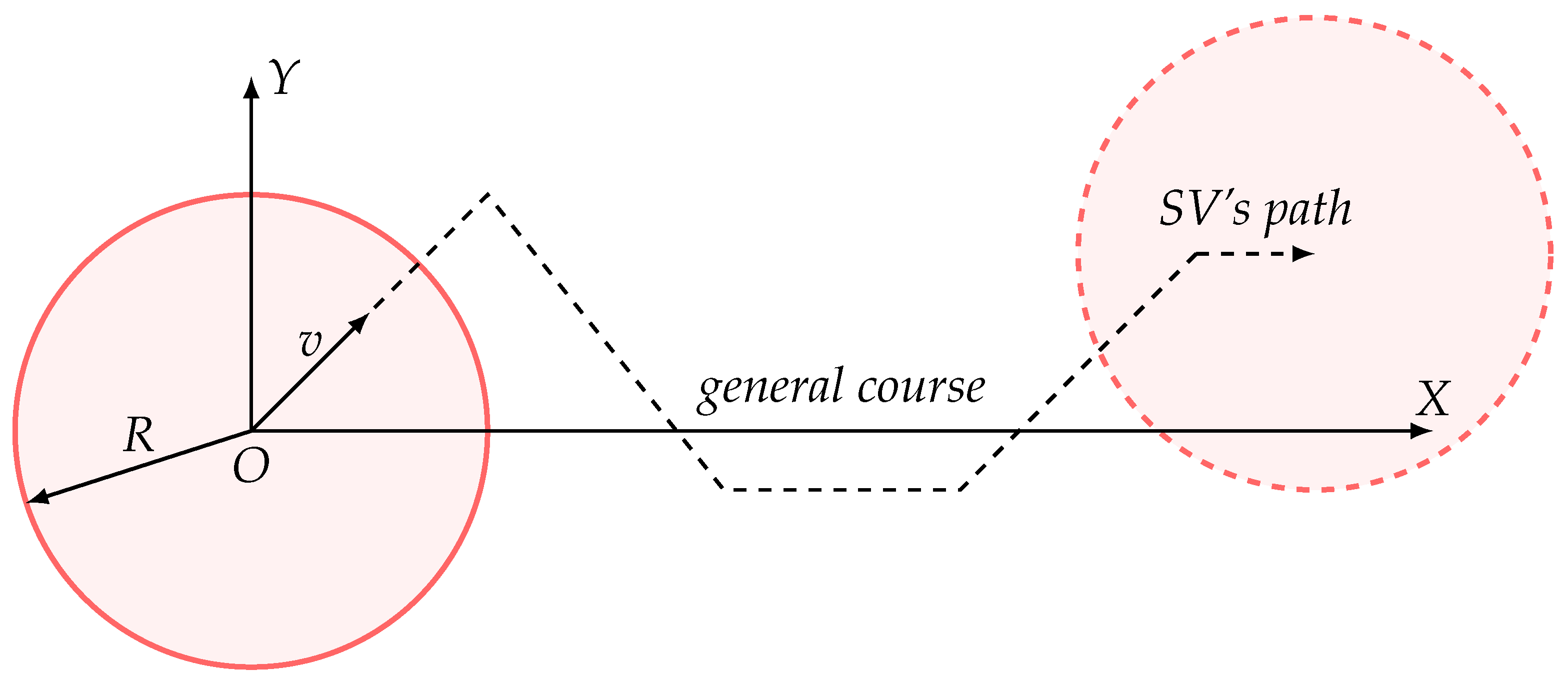
2. Model of the SV’s Movement on Tacks

The search system consists of one SV, which has a circle detection zone of radius R. The SV moves piecewise-rectilinearly on a plane, tacking randomly around the line of the general course. The origin O of the stationary Cartesian coordinate system $XOY$ is situated in the initial position of the SV, as shown in Figure 1. This coordinate system is oriented in such a way that its $OX$ axis coincides with the line of the general course of the SV.

The SV moves on tacks in accordance with the following law:

$$\left\{\begin{array}{c}{\displaystyle {\dot{x}}_{SV}=v_x=vcos\alpha ,}\hfill \\ {\displaystyle {\dot{y}}_{SV}=v_y={\theta }_{t}vsin\alpha ,}\hfill \end{array}\right.$$

(1)

where $\alpha$ is the specified tacking angle, v is the SV’s search speed, and ${\theta }_t$ is a random jump-like Markov process. The component of the SV’s velocity vector $\overrightarrow{v}$ along the line of the general course is constant:

$$v_x=\mathrm{const}.$$

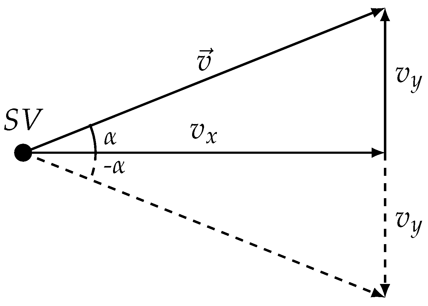
Figure 2 shows a velocity diagram of the SV. As follows from (1), tacking was performed by periodically changing the velocity component $v_y$ according to a random Markov process ${\theta }_t$ with a finite vector of states $J=(j_1,j_2,\dots ,j_n)$ and a given matrix of the transition intensities between these states $\Lambda$. This article discusses the case of processes with three states $J=(-1,0,1)$. This means that the SV’s velocity vector can coincide with the general course line (${\theta }_t=0$) or deviate from it by a constant angle equal to $\pm \alpha$ (when ${\theta }_t=\pm 1$), as shown in Figure 2.

We considered transitions between process states equally possible with transition intensity matrix:

$$\Lambda =\lambda \left(\begin{array}{ccc}\hfill -2& \hfill 1& \hfill 1\\ \hfill 1& \hfill -2& \hfill 1\\ \hfill 1& \hfill 1& \hfill -2\end{array}\right),$$

(2)

corresponding to the state vector J. The variable $\lambda$ here is $\lambda =1/{\tau }_0$, where ${\tau }_0$ is the average time of the SV being on one tack. This model generates random trajectories that have the approximate shape shown in Figure 1.

For the mathematical formulation of the stochastic optimization problem, it is convenient to study the Gaussian Markov analog instead of the jump-like process ${\theta }_t$. This diffusion process ${\Theta }_t$ has the same mathematical expectation and correlation function as the process ${\theta }_t$. It follows from the theory of jump-like Markov processes that ${\Theta }_t$ allows the stochastic Ito differential [30]:

$$d{\Theta }_t=-D{\Theta }_{t}dt+\sigma d{w}_t,$$

(3)

where $w_t$ is a standard Wiener process and $D,\sigma$ are constants related to the original Markov process ${\theta }_t$: $D\triangleq 3\lambda$ and $\sigma \triangleq 2tan\alpha \sqrt{\lambda }$.

3. Detection Probability of the SO Moving at a Constant Velocity

Firstly, let us consider the task of detecting a target SO (target) with the SV, whose dynamics is described in Section 2. The following model was investigated. The target moves at a constant speed parallel to the general course line of the SV at a distance l from it.

The initial distance between the vehicles along the general course is L, so the initial Cartesian distance is ${\displaystyle \sqrt{L^2+l^2}}$. The SV is moving according to (1), where ${\theta }_t$ is a random Markov process with the state vector J and the transition matrix $\Lambda$ from (2). The target moves according to the law:

$$\left\{\begin{array}{c}{\displaystyle \dot{x}=-u,}\hfill \\ {\displaystyle \dot{y}=0,}\hfill \end{array}\right.$$

(4)

where u is its constant velocity.

The target will be detected if the distance between it and the SV becomes less than R. To simplify the model, let us assume that the detection is successful when the target’s and SV’s x-coordinates become equal at some point in time: $x_{SV}\left(\vartheta \right)=x\left(\vartheta \right)$, and the inequality $|y_{SV}\left(\vartheta \right)-y\left(\vartheta \right)|\le R$ is satisfied for the y coordinates.

The rendezvous instant $\vartheta$ is defined as:

$$\vartheta =\frac{L}{vcos\alpha +u}.$$

(5)

The probability of detection will be determined by including the $y_{SV}$ coordinate in the interval $[l-R,l+R]$, namely:

$${\mathbf{P}}_{\det }=\mathbf{P}\{l-R\le y_{SV}\left(\vartheta \right)\le l+R\}=\mathbf{P}\left\{\frac{l-R}{vsin\alpha }\le {\int }_0^{\vartheta }{\theta }_{s}ds\le \frac{l+R}{vsin\alpha }\right\}.$$

(6)

As mentioned in (3), the random jump-like Markov process ${\theta }_t$ can be replaced with its Gaussian Markov analog ${\Theta }_t$, which has the same mathematical expectation and correlation function as the process ${\theta }_t$.

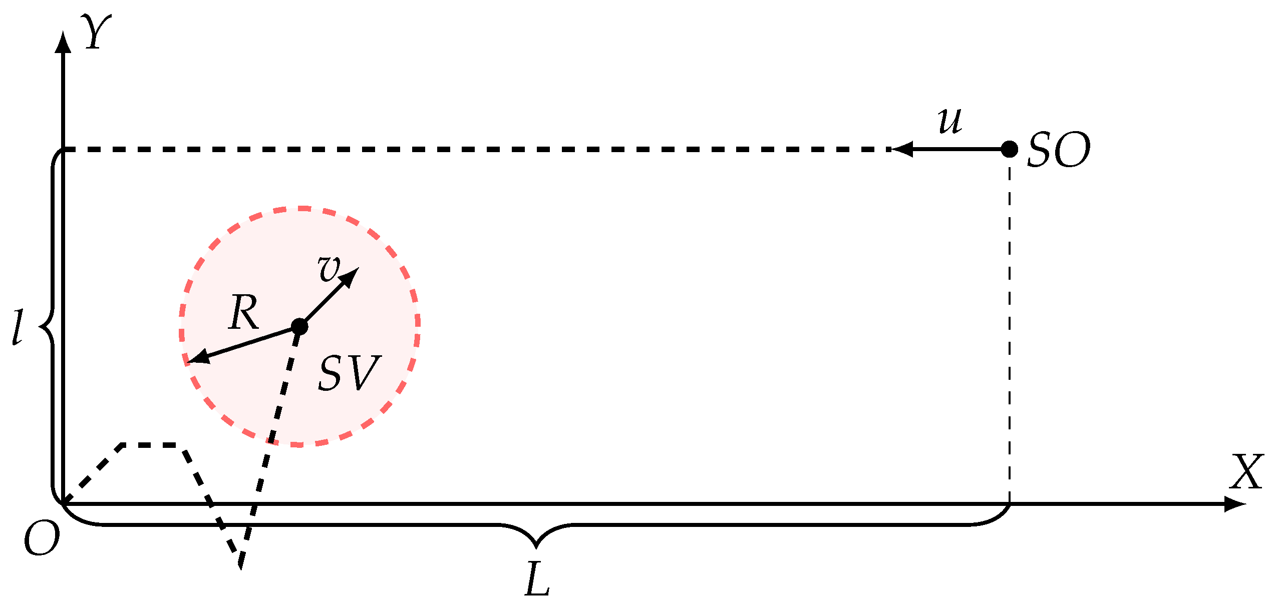
Further, instead of calculating the random integral (6), we estimated the target detection probability by the SV through the analytical approximation of probability histograms, obtained in the numerical simulation. We assumed that at the instant $t_0=0$, the target is situated in the position $E^0=(L,l)$ and $L\gg 1$ (as shown in Figure 3) and the velocity of the target $u<1$.

Due to the latter assumption, the SV’s detection zone can be considered as a flat-line segment with the length of the diameter instead of the circle. Thus, the detection probability can be estimated as the probability of meeting the target with this segment.

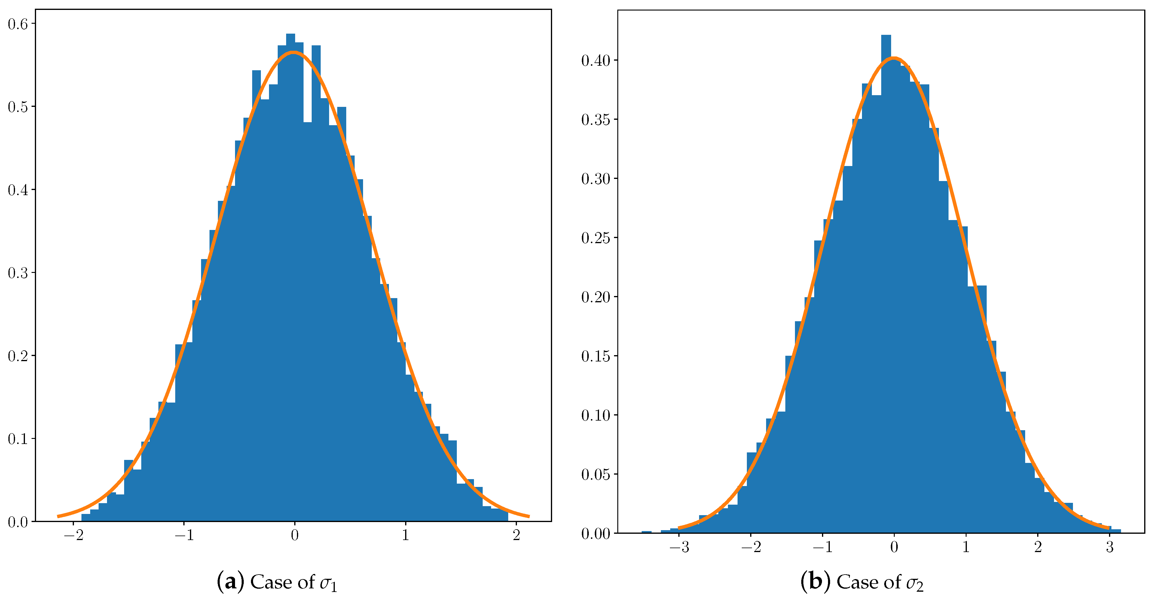
The histograms of the distribution density of the $y_{SV}$ coordinate obtained in the interval $[l-\Delta l,l+\Delta l]$ for some small $\Delta l$ are well approximated by the symmetric density of the Gaussian distribution. Figure 4 depicts the histogram of the probability of meeting between the target and SV and the corresponding density of the Gaussian distributions: $\mathcal{N}(0,{\sigma }_1^2)$ for ${\sigma }_1=0.705$ for the case $L=L_1=5$ (Figure 4a) and $\mathcal{N}(0,{\sigma }_2^2)$ for ${\sigma }_2=0.993$ for the case $L=L_2=10$ (Figure 4b). The histograms were constructed as a result of computer simulation of the movement of the target and SV for 10,000 implementations of the SV trajectory corresponding to $\lambda =5/3$.

These graphs allowed us to estimate the SV’s detection probability ${\mathbf{P}}_{\det }$ at its various initial positions. Now, Equation (6) may be approximated as:

$${\mathbf{P}}_{\det }=\mathbf{P}\{l-R\le y_{SV}\left(\vartheta \right)\le l+R\}=\frac{1}{\sqrt{2\pi }{\sigma }_i}{\int }_{l-R}^{l+R}exp\left(-y^2/\left(2{\sigma }_i^2\right)\right)dy,$$

(7)

where ${\sigma }_i$ corresponds to various parameters $(L_i,l_i,u_i)$. In particular, when $l=l_1=1.5$ and $l=l_2=2.5$ for $L_1$ and $L_2$, respectively, these probabilities are presented in

Table 1. The detection probability of the target ${\mathbf{P}}_{\det }$ at its various initial positions $E^0=(L,l)$.

L	l	${\mathbf{P}}_{\mathbf{det}}$
5	1.5	0.238
5	2.5	0.017
10	1.5	0.304
10	2.5	0.065

. In all cases, the velocity of the target is $u=0.3$. All values are given in a normalized scale.

Next, we introduced a certain threshold value (security threshold) $h<1$ of the permissible detection probability of ${\mathbf{P}}_{\det }$, for example $h=0.07$. The situation with ${\mathbf{P}}_{\det }\le h$ is considered safe. In this case, the target continues to move in a straight line without changing its course and speed. If ${\mathbf{P}}_{\det }>h$, then the situation is considered dangerous. It was assumed that in the case of a dangerous situation, the target (to prevent the negative consequences of possible detection) uses the mobile defender mentioned in the Introduction, whose task is to intercept the SV with a minimum standard error at a given point in the plane relative to the SV.

The minimization of this miss is associated with the solution of the following optimal stochastic control problem.

4. Optimal Stochastic Control Problem

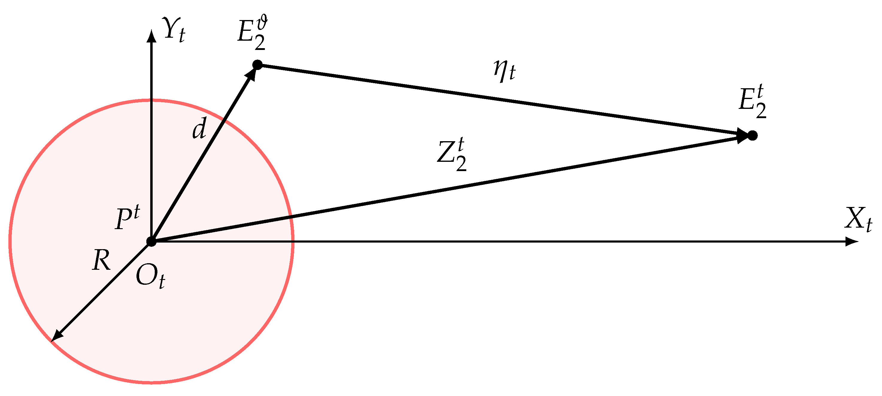
The problem was considered in a moving Cartesian coordinate system $X_t{O}_t{Y}_t$, where the origin $O_t$ is associated with the current position $P^t$ of the SV and the axis $O_t{X}_t$ is directed parallel to the SV’s general course. The current position of the defender $E_2^t$ is given by a two-dimensional vector $Z_2^t$ directed from $O_t\triangleq P^t$ to $E_2^t$.

Terminal position $E_2^{\vartheta }$ of the defender is defined by a given two-dimensional vector d, as shown in Figure 5. An auxiliary vector ${\eta }_t\triangleq Z_2^t-d$ was introduced for a more convenient formulation of the defender’s optimal control problem.

In the selected coordinate system, the equations of the relative motion of the defender–SV system have the form:

$${\dot{Z}}_2^t=u_t-\left(\begin{array}{c}1\\ {\Theta }_t\end{array}\right),u_t=\left(\begin{array}{c}{u}_x^t\\ u_y^t\end{array}\right),$$

(8)

where ${\Theta }_t$ is from (3) and the initial position of $Z_2^0$ were set. The two-dimensional velocity vector $u_t$ of the defender plays the role of the control and is subject to the restrictions:

$$|u_t|\le \beta <1$$

(9)

with the specified constant $\beta$.

In terms of the auxiliary vector ${\eta }_t$ introduced above, the equations of motion (8) take the compact form:

$${\dot{\eta }}_t=u_t+A+B{\Theta }_t,{\eta }_0\triangleq Z_2^0,$$

(10)

where:

$$A=\left(\begin{array}{c}\hfill -1\\ \hfill 0\end{array}\right),B=\left(\begin{array}{c}\hfill 0\\ \hfill -1\end{array}\right).$$

(11)

At the terminal moment $\vartheta$, the following condition must be met:

$$\mathbf{E}{\eta }_{\vartheta }=0,$$

(12)

where $\mathbf{E}$ is the sign of the mathematical expectation. As a criterion, we took the terminal functional:

$$\mathbf{E}G({\eta }_{\vartheta },{\Theta }_{\vartheta })\to \underset{u_t}{min},$$

(13)

where:

$$G({\eta }_{\vartheta },{\Theta }_{\vartheta })={\eta }_{\vartheta }^2+\gamma {\Theta }_{\vartheta }.$$

(14)

In (13) and (14), the summand ${\eta }_{\vartheta }^2$ characterizes the standard deviation of the defender from the end of the vector d at the terminal moment $\vartheta$. The term $\gamma \mathbf{E}{\Theta }_{\vartheta }$, where $\gamma$ is a given constant, plays the role of an additional terminal penalty for the “convenient” or “inconvenient” tack of the SV at the time of $\vartheta$. Here, the words “convenient” or “inconvenient” are used in the following sense. The tack of the SV at the time of $\vartheta$ is considered “convenient” if ${\Theta }_{\vartheta }<0$, i.e., the component of the velocity of the SV along the $OY$ axis is negative (the SV is moving away from the line of the movement of the target $E_1$). Otherwise, we considered the tack of the SV “inconvenient”.

5. Optimal Stochastic Control

5.1. Reduction of the Optimal Stochastic Control Problem to the Deterministic One

It is known that solving stochastic optimization problems in real time is associated with certain difficulties [30]. For this reason, instead of the original stochastic problem (3), (9)–(14), we solved its deterministic analog. To construct this analog, we need the following auxiliary results.

The solution of Equation (3) has the form:

$${\Theta }_t=e^{-Dt}{\Theta }_0+\sigma {\int }_0^t{e}^{-D(t-s)}d{w}_s.$$

(15)

Integration (15) leads to the equation:

$${\int }_0^t{\Theta }_{s}ds=\frac{{\Theta }_0}{D}\left(1-e^{-Dt}\right)+\frac{\sigma }{D}{\int }_0^t\left(1-e^{-D(t-s)}\right)d{w}_s.$$

(16)

Now, let us calculate the value of the criterion (13) with an arbitrary permissible program control $u_t$ and the parameter $\vartheta$ fixed at the moment $t_0=0$. To this end, we integrated the equations of motion (10) taking into account (16). We have:

$${\eta }_{\vartheta }={\eta }_0+A\vartheta +B\frac{{\theta }_0}{D}\left(1-e^{-D\vartheta }\right)+B\frac{\sigma }{D}{\int }_0^{\vartheta }\left(1-e^{-D(\vartheta -s)}\right)d{w}_s+{\int }_0^{\vartheta }{u}_{s}ds.$$

(17)

From (12) and (17) follows:

$$\mathbf{E}{\eta }_{\vartheta }={\eta }_0+A\vartheta +B\frac{{\Theta }_0}{D}\left(1-e^{-D\vartheta }\right)+{\int }_0^{\vartheta }{u}_{s}ds=0.$$

(18)

Finally, from (17) and (18), we obtain:

$$\mathbf{E}{\eta }_{\vartheta }^2=\frac{{\sigma }^2}{D^2}\left[\vartheta -\frac{2}{D}\left(1-e^{-D\vartheta }\right)+\frac{1}{2D}\left(1-e^{-2D\vartheta }\right)\right].$$

(19)

Thus, the (13) criterion takes the form:

$$\mathbf{E}G=\frac{{\sigma }^2}{D^2}\left[\vartheta -\frac{2}{D}\left(1-e^{-D\vartheta }\right)+\frac{1}{2D}\left(1-e^{-2D\vartheta }\right)\right]+\gamma e^{-D\vartheta }{\Theta }_0\to \underset{u_t}{min}.$$

(20)

Now, we transformed (18) by introducing a two-dimensional vector ${\xi }_t$ subordinate to the equation:

$${\dot{\xi }}_t=A+B{\Theta }_0{e}^{-Dt}+u_t$$

(21)

with boundary conditions:

$${\xi }_0={\eta }_0,{\xi }_{\vartheta }=0.$$

(22)

In terms of the vector ${\xi }_t$, the desired deterministic analog is the following auxiliary problem of optimal (deterministic) control, which includes the equations of motion (21), boundary conditions (22), control constraints (9), and terminal criterion $F\left(\vartheta \right)\to \underset{u_t}{min}$, where $F\left(\vartheta \right)$ denotes the right-hand side of (20) with the excluded additive constants $-2{\sigma }^2/D^3$ and ${\sigma }^2/\left(2D^3\right)$:

$$F\left(\vartheta \right)\triangleq \frac{{\sigma }^2}{D^2}\left[\vartheta +\frac{2}{D}{e}^{-D\vartheta }-\frac{1}{2D}{e}^{-2D\vartheta }\right]+\gamma e^{-D\vartheta }{\Theta }_0\to \underset{u_t}{min}.$$

(23)

5.2. Pontryagin’s Maximum Principle in the Auxiliary Optimal Problem (23)

To solve the auxiliary problem, we used Pontryagin maximum principle (PMP) [31]. According to the procedure of PMP, firstly, we constructed the Hamiltonian:

$$H={\lambda }_{\xi }·\left(A+B{\theta }_0{e}^{-Dt}\right)+{\lambda }_{\xi }·u_t\to \underset{u_t}{max}.$$

(24)

Here, the dot between the two-dimensional vectors means a scalar product, and ${\lambda }_{\xi }={\lambda }_{\xi }\left(t\right)$ is a conjugate variable corresponding to the phase variable ${\xi }_t$. From (24), we found the explicit form of the optimal control (here and further, the * symbol indicates the optimal controls):

$${\displaystyle u_t^{*}=\beta \frac{{\lambda }_{\xi }\left(t\right)}{|{\lambda }_{\xi }\left(t\right)|}.}$$

(25)

The conjugate variable satisfies [31]:

$${\displaystyle {\dot{\lambda }}_{\xi }\left(t\right)=-\frac{\partial H}{\partial \xi }\left(t\right)=0;}$$

(26)

hence ${\lambda }_{\xi }\left(t\right)={\lambda }_{\xi }=\mathrm{const}$, which leads to $u_t^{*}=u^{*}=\mathrm{const}$ with $|u^{*}|=\beta$. In other words, the program motion of the controlled object is implemented in a straight line with the maximum possible speed. The transversality conditions at instant $\vartheta$ are given by:

$$\delta F\left(\vartheta \right)+{\lambda }_{\xi }·\delta \xi -H\delta \vartheta =0,$$

(27)

where according to (23):

$${\displaystyle \delta F\left(\vartheta \right)=\frac{\partial F\left(\vartheta \right)}{\partial \vartheta }\delta \vartheta =\frac{{\sigma }^2}{D^2}\left[1-2e^{-D\vartheta }+e^{-2D\vartheta }\right]\delta \vartheta -\gamma D{e}^{-D\vartheta }{\theta }_0\delta \vartheta .}$$

(28)

Following (27), (28):

$${\displaystyle H\left(\vartheta \right)=\frac{{\sigma }^2}{D^2}\left[1-2e^{-D\vartheta }+e^{-2D\vartheta }\right]-\gamma D{e}^{-D\vartheta }{\theta }_0.}$$

(29)

Integrating (21), taking into account (22), gives:

$${\displaystyle {\eta }_0+A\vartheta +B\frac{{\theta }_0}{D}\left(1-e^{-D\vartheta }\right)+u^{*}\vartheta =0}$$

(30)

that naturally coincides with (18) under $u_t=u^{*}$.

Next, we put

$$\left\{\begin{array}{c}{u}^{*}\triangleq \beta (cos\phi ,sin\phi ),\mathrm{with}\phi =\mathrm{const},\hfill \\ {\eta }_0\triangleq (x_0,y_0).\hfill \end{array}\right.$$

(31)

Then, from (30) and (31), we have in a componentwise form of the system of two equations with respect to $\phi$ and $\vartheta$:

$$\left\{\begin{array}{c}{x}_0-\vartheta +\beta \vartheta cos\phi =0,\hfill \\ {\displaystyle y_0+\beta \vartheta sin\phi -\frac{{\theta }_0}{D}\left(1-e^{-D\vartheta }\right)=0.}\hfill \end{array}\right.$$

(32)

From (32) follows:

$$\left\{\begin{array}{c}cos\phi =(\vartheta -x_0){\left(\beta \vartheta \right)}^{-1},\hfill \\ {\displaystyle sin\phi =\left[\frac{{\Theta }_0}{D}\left(1-e^{-D\vartheta }\right)-y_0\right]{\left(\beta \vartheta \right)}^{-1},}\hfill \end{array}\right.$$

(33)

where $\vartheta$ can be found as the least-positive root of the equation, following from the identical equality ${cos}^2\phi +{sin}^2\phi =1$ with respect to the right parts of (33), namely:

$${(\vartheta -x_0)}^2+{\left[{\displaystyle \frac{{\Theta }_0}{D}\left(1-e^{-D\vartheta }\right)-y_0}\right]}^2={\beta }^2{\vartheta }^2.$$

(34)

Formulas (33) and (34) allow us to find the velocity components of the controlled object and the time interval $[0,\vartheta ]$ of its motion from the initial position to the end of the vector d.

If $D\vartheta$ in (34) is sufficiently large, then the term $e^{-D\vartheta }$ is close to zero and can be omitted. In this case, (34) takes the form:

$${(\vartheta -x_0)}^2+{\left({\displaystyle \frac{{\Theta }_0}{D}-y_0}\right)}^2={\beta }^2{\vartheta }^2.$$

(35)

Then, the instant $\vartheta$ can be found as the least root of the square Equation (35):

$${\displaystyle \vartheta =\frac{x_0-\sqrt{x_0^2-\left(1-{\beta }^2\right)\left(x_0^2+{\left({\displaystyle \frac{{\Theta }_0}{D}-y_0}\right)}^2\right)}}{1-{\beta }^2}.}$$

(36)

To construct a positional optimal control (feedback control) of the defender, the current moment t was taken as the initial $t_0$, the current position $(x_t,y_t)$ was taken as the initial $(x_0,y_0)$, and the current value of ${\Theta }_t$—for the initial ${\Theta }_0$; after that, the instantaneous direction of the vector $u_t^{*}$ of the defender’s velocity was calculated using the formulas (31) taking into account (33) and (36). Next, $u_t^{*}$ was recalculated at the rate of updating the current information. Note that at a high rate of updating this information, it may be quite justified to use the piecewise program control of the defender, in which its control is recalculated only at certain moments called correction moments with intervals between them $\Delta t_u$. During these intervals, the defender moves programmatically according to control $u_t^{*}$, calculated in the previous step.

6. Examples

To demonstrate the effectiveness of the obtained optimal control, a numerical simulation was performed for two approaches for studying the interaction between the defender and SV. These approaches differ in the mathematical description of the evolution of the y-component of the SV’s velocity. In the first (discrete) approach, this component is piecewise constant and its evolution is described as a jump-like Markov process ${\theta }_t$ with three states $(1,0,-1)$ and the transition intensity matrix $\Lambda$ from (2). The description of this process is given in the beginning of Section 2. In the second (continuous) approach, an evolution of the y-component of the SV’s velocity vector is set by Gaussian process ${\Theta }_t$, i.e., continuous diffusion process (3).

In both approaches, the control of the defender was obtained through Equations (31), (33), and (36). In other words, the control of the defender is always calculated according to the continuous diffusive model (3) of the evolution of the y-component of the SV’s velocity vector. Strictly speaking, as this control law is the result of the solution of the continuous problem, it should not always successfully solve the discrete problem, simulated in the first approach. The idea of these experiments is to apply the solution of the continuous problem, which can be solved analytically, to the similar discrete practical model, which cannot be studied in the same convenient way. In all experiments, vector d was considered to be null, i.e., the defender has to intercept the SV.

Both approaches to the simulation are shown in further examples, which were devoted to two different applications of the studied interception problem.

The realization of diffusive process ${\Theta }_t$ was acquired in Maple with the package for stochastic equations. An approximate formula for $\vartheta$ (36) was used for the stochastic differential Equation (15). Thus, Maple allows integrating this equation numerically and obtaining the optimal trajectory of the defender, as well as the random trajectory of the SV corresponding to the process with the appropriate mathematical expectation and dispersion.

A more practical discrete jump-like process ${\theta }_t$ was simulated in Python script. The movement of the SV and defender was computed with a very small discretization step $\Delta t$, which is the quality of the simulation. At each step, the SV, according to the model from Section 3, can change the direction of its $v_y$ velocity component with probability $2\lambda \Delta t$ or not change it with probability $(1-2\lambda \Delta t)$. However, in practice, this model is not very useful. This process is identical to a Gaussian process: the time of another SV tack is sampled exponentially with mathematical expectation $1/\lambda$, and the direction of the vertical velocity for this tack is chosen from two directions, different from the current one with probability $1/2$. The defender, on the other hand, has its own parameter $\Delta t_u$ and corrects its control law according to (36) every interval $\Delta t_u$, considering the current positions to be initial.

6.1. Intrusion in the Detection Zone

The first application is the intrusion of the SV’s detection zone by the defender to distract the SV from the target. In normalized scale, these parameters are:

$$R=1,v_x=1,{\tau }_o=0.6.$$

Let ${\displaystyle tan\alpha =0.5}$. Then, the parameters for Gauss process ${\Theta }_t$ are:

$$\lambda =\frac{1}{{\tau }_0}\approx 1.67,D=3\lambda \approx 5,\sigma =2tan\alpha \sqrt{\lambda }=1.29.$$

In the coordinate system associated with the initial position of the SV, the initial coordinates of the defender’s position are $(10,1)$ in the normalized scale. The velocity of the defender was chosen as $\beta =0.5$. The probability of the detection of the target following a parallel course from this coordinates equals ${\mathbf{P}}_{\det }=0.5$, which is higher than the accepted security threshold $h=0.07$. Thus, according to the above-described security concept, the target must use a mobile defender.

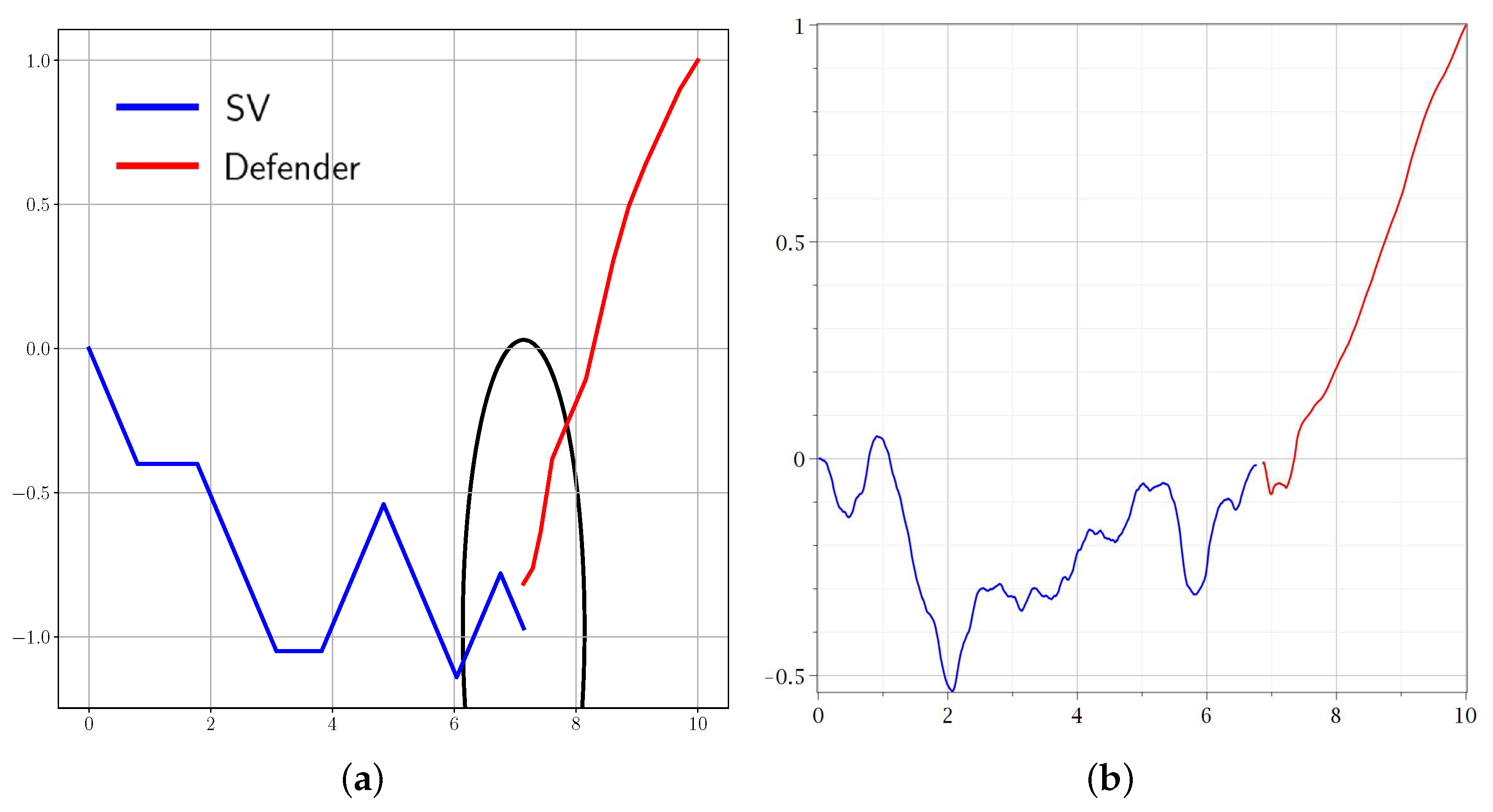
The results of this experiment are shown in Figure 6. The red line depicts the trajectory of the defender, whereas the blue one, that of the SV. Figure 6a shows the evolution of the y-component of the SV’s velocity according to Markov jump-like process ${\theta }_t$. Figure 6b shows the trajectories of the vehicles for the diffusion approximation ${\Theta }_t$ of the process ${\theta }_t$. In Figure 6a, the black ellipse depicts the circular detection zone of radius R, which looks ellipsoidal due to the different scale of the $OX$ and $OY$ axes. In the case of the discrete model, the parameter $\Delta t_u$ is equal to ${\tau }_0$. In the case of the continuous model, the calculation of the defender’s optimal control is performed in time with the SV’s information updating, i.e., almost continuously ($\Delta t_u$ equals the simulation discretization step).

For the estimation of time $\vartheta$, Equation (36) was used. According to (36), interception time $\vartheta =7$, which means ${\displaystyle e^{-D\vartheta }\approx 0}$, i.e., ${\displaystyle 1-e^{-D\vartheta }\approx 1}$, so $u_t$ can be found from Equations (31), (33), and (36). One can see in Figure 6 that the trajectories of the defender for the discrete and continuous models of the SV’s movement were quite close. The difference of the trajectories in the final sections was due to the significant duration of the interval $\Delta t_u$ between the updates of the information about the SV and, thereby, the corrections of the defender’s program control in the discrete approach.

As one can see, the problem of interception was solved successfully, as the defender moving from the initial position with the found u control finally occurred in the close vicinity of the SV.

6.2. Destruction of the SV

The second application is the task of the destruction of the SV using the defender. To complete this task, the defender must come close enough to the SV. In the normalized scale:

$$R=1,v_x=1,{\tau }_o\approx 60.$$

Let $tan\alpha =0.5$. Therefore:

$$\lambda =0.017,D=0.05,\sigma =0.13.$$

In the coordinate system associated with the initial position of the SV, the initial coordinates of the defender are $(300,20)$ in the normalized scale. The velocity of the defender was chosen as $\beta =0.5$. As the target moves parallel to the general course of the SV, then the detection probability ${\mathbf{P}}_{\det }$ equals ${\mathbf{P}}_{\det }=0.37>h=0.07$; thus, using the defender is justified.

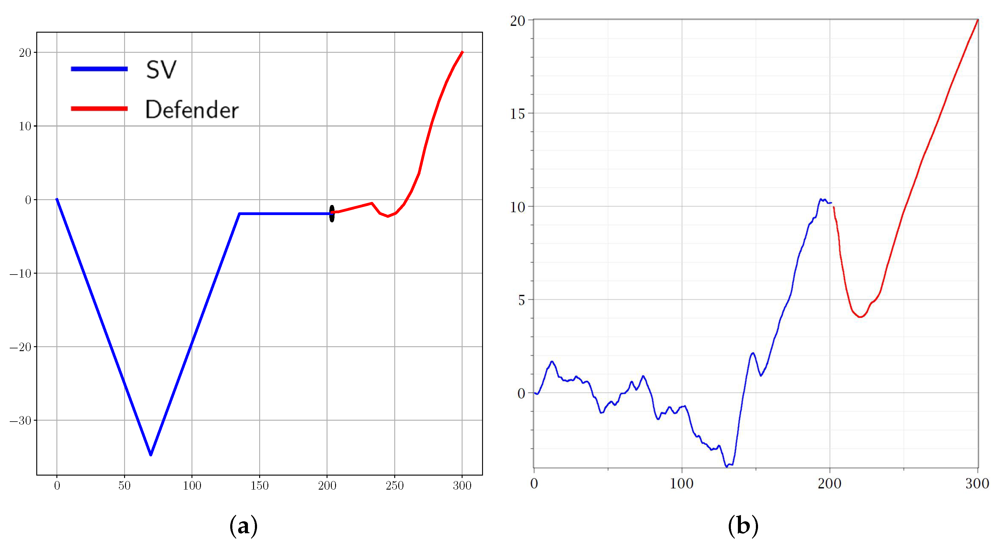
The results of the modeling are presented in Figure 7. As in the first example, Figure 7a corresponds to the discrete approach to the simulation and the process ${\theta }_t$, and Figure 7b relates to the continuous approach and the process ${\Theta }_t$.

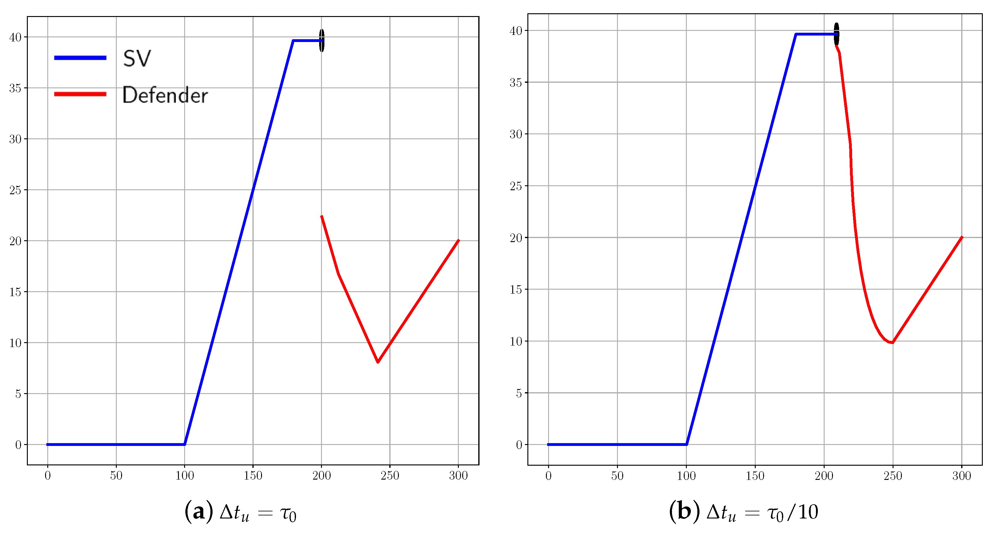
The accuracy of the interception of the SV by the defender or the so-called terminal miss obviously depends on the parameter $\Delta t_u$—the time interval between corrections of the defender’s control. Figure 8 presents the results of different simulations of the interception of the SV by the defender for the discrete approach. Figure 8a corresponds to the case of $\Delta t_u={\tau }_0$. A sufficient miss of the defender can be explained by the relatively significant duration $\Delta t_u$ of its movement without control correction and the “inconvenient” realization of the tack, which combined with the velocity advantage ($\beta <1$) allowed the SV to avoid interception by the defender. However, decreasing the parameter $\Delta t_u$ helped achieve more satisfactory results, as shown in Figure 8b. For two similar realizations of process ${\theta }_t$ (blue lines), the trajectories of the controlled defender (red lines) were clearly very different with dependence on the parameter $\Delta t_u$ (${\tau }_0$ and ${\tau }_0/10$, respectively).

6.3. Comparison with Classic Guidance Methods

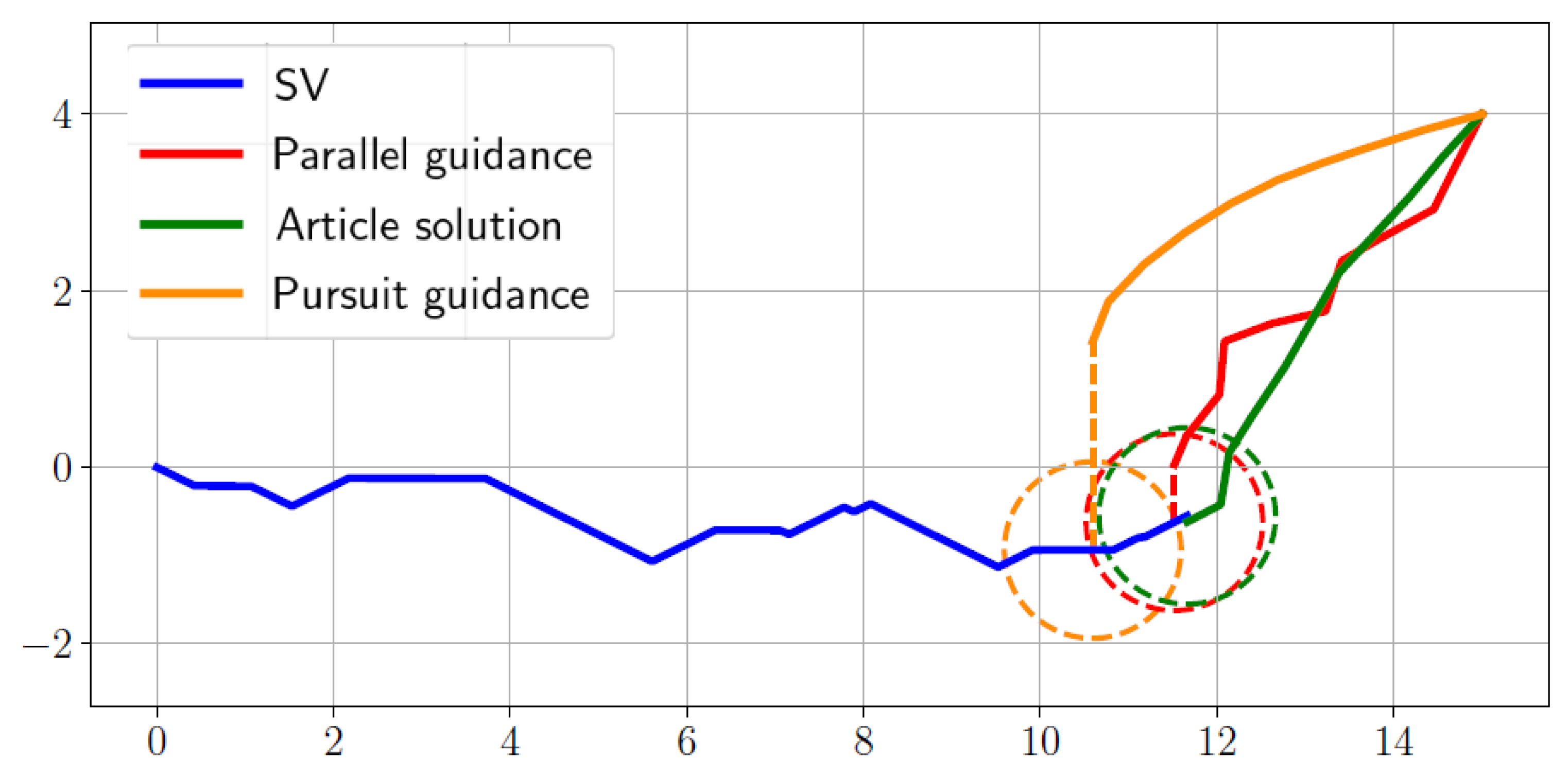
The optimal control law of the defender obtained here was compared with classic guidance methods, mentioned in the Introduction, such as the pursuit guidance method and parallel guidance, which is a specific case of the proportional navigation guidance method. On average, our method gave better results than the others. In Figure 9, a typical realization of different simulated guidance methods is presented. The orange line designates the trajectory of the defender, acting according to the pursuit guidance method; the red line denotes the trajectory generated by the parallel guidance algorithm; the blue graph shows the SV’s movement. The defender, controlled according to Equations (31), (33) and (36), has a green trajectory. Dashed lines illustrate the distances on the Y axis between the SV and defender at instant $\vartheta$ when their X-coordinates coincide.

As one can see, the green defender was closer to the SV than the others. Classic guidance methods are effective when the pursuer velocity is higher than the one of the evader. That is not the case in the current study, because the defender’s velocity $\beta$ was less than the velocity of the SV. Moreover, the classic guidance methods are not intended to be use for intercepting stochastic targets, unlike the control law obtained in this article as a solution of the stochastic optimal control problem.

7. Conclusions

The article considered one “attacker–target–defender”-type problem of the interaction on a plane between the search system, consisting of one search vehicle with the circle detection zone, and the mobile searched object. The search vehicle tacked randomly along a given general course towards the searched object, and its movement was described using a Markov jump-like process. The searched object had a mobile defender onboard, which can be used for the distraction and destruction of the search vehicle, if it presents a danger to the searched object in the sense of its detection. The feature of this problem is that the defender has lower dynamic capabilities in comparison to the searching vehicle being intercepted.

It was shown that, being stochastic in nature, the optimal control problem of the interception of a search vehicle can be transformed into the classic deterministic problem of optimal control in the class of piecewise-programmatic controls. The optimal time of interception was estimated, and an optimal control law was found. The examples of the numerical simulations for both the discrete and continuous (stochastic and deterministic) problems were presented to reveal the efficiency of the designed results. Furthermore, a comparison with the interception solutions, based on classic guidance laws, was presented.

In the future, it is planned to consider a similar problem statement with a group of search vehicles instead of one.