Article

H and Passive Fuzzy Control for Non-Linear Descriptor Systems with Time-Varying Delay and Sensor Faults

1
Department of Industrial Engineering, College of Engineering, University of Hail, Hail 2440, Saudi Arabia
2
Department of Electrical Engineering, College of Engineering, University of Hail, Hail 2440, Saudi Arabia
3
Lab-STA, LR11ES50, National School of Engineering of Sfax, University of Sfax, Sfax 3038, Tunisia
4
Department of Computer Engineering, College of Computer Science and Engineering, University of Hail, Hail 2440, Saudi Arabia
5
Faculty of Electrical and Control Engineering, Gdansk University of Technology, ul. Narutowicza 11/12, 80-233 Gdańsk, Poland
*
Author to whom correspondence should be addressed.
Mathematics 2021, 9(18), 2203; https://doi.org/10.3390/math9182203
Submission received: 20 August 2021 / Revised: 31 August 2021 / Accepted: 3 September 2021 / Published: 8 September 2021
(This article belongs to the Special Issue Fuzzy and Extension of Fuzzy Theories)

Abstract

:
In this paper, the problem of reliable control design with mixed H /passive performance is discussed for a class of Takagi–Sugeno TS fuzzy descriptor systems with time-varying delay, sensor failure, and randomly occurred non-linearity. Based on the Lyapunov theory, firstly, a less conservative admissible criterion is established by combining the delay decomposition and reciprocally convex approaches. Then, the attention is focused on the design of a reliable static output feedback (SOF) controller with mixed H /passive performance requirements. The key merit of the paper is to propose a simple method to design such a controller since the system output is subject to probabilistic missing data and noise. Using the output vector as a state component, an augmented model is introduced, and sufficient conditions are derived to achieve the desired performance of the closed-loop system. In addition, the cone complementarity linearization (CCL) algorithm is provided to calculate the controller gains. At last, three numerical examples, including computer-simulated truck-trailer and ball and beam systems are given to show the efficacy of our proposed approach, compared with existing ones in the literature.

1. Introduction

Descriptor systems are recognized as a powerful mathematical model able to describe the dynamic behavior as well as the interconnection properties of many practical plants [1,2]; also referred to as singular systems, descriptor systems have known many applications in the fields related to electrical circuits, large-scale interconnected systems, electromechanical and constrained mechanical systems, economy, and biological systems. Due to its impulse behavior, this class of systems has received many research works [3,4]. Particularly, the discrete descriptor systems have received a great deal of attention and many research value in asymptotic stability, regularity and causality have been published in the literature [5,6,7,8,9,10,11]. On another hand, it is well known that time delay is ubiquitous in various engineering systems and it is the main cause of instability and performance degradation of dynamic systems. Consequently, the study of descriptor systems with delays has attracted lots of researchers’ attention [12,13,14]. Based on the LMI approach, the direct Lyapunov method is generally used for investigating the admissibility condition for discrete-time descriptor systems with time-varying delay. Many works have been done on this topic. By taking advantage of the delay partitioning technique, a delay-dependent admissibility criterion was developed in [8]. Recently, the reciprocally convex combination method was investigated in [10] to derive a less conservative admissibility criterion. In [11], a new summation inequality, which is less conservative than the usual Jensen inequality, was introduced and utilized to analyze the admissibility problem. Usually, employing the reciprocally convex combination approach or the delay decomposition approach yields less conservative results. This motivates us to combine both approaches to revisit the admissibility condition of discrete-time descriptor delay systems.
On another research front, the analysis and design of non-linear systems is one of the most challenging issues in systems and control theory. Recently, Takagi–Sugeno TS fuzzy model was proved to be a powerful and promising method to approximate non-linear plants in applications [15,16]. In this context, the sector non-linearity approach was extensively used as a systematic method to derive an equivalent TS fuzzy model of the original non-linear system [17]. A shortcoming of this approach is that the fuzzy rules number increases exponentially with the number of non-linearities arising from the original systems, leading to increased computational costs. Benefiting from these models, many results are dedicated for non-linear descriptor systems with time delay. In the quoted papers, the admissibility analysis for discrete and continuous fuzzy descriptor systems were addressed [6,18]. For discrete-time fuzzy singular systems subject to actuator saturation, passive and H  control schemes were addressed in [19,20], respectively. A second motivation of this paper is to benefit from this model to describe the system under consideration.
To keep the controlled systems less sensitive to external disturbances, a great deal of attention has been dedicated to the H  control theory. Furthermore, the passivity, which is defined in terms of energy dissipation and transformation, was investigated in control engineering to deal with robust stability problems for different classes of systems, such as networked control systems [21], fuzzy systems [22], signal processing systems [23], and stochastic systems [24]. Very recently, the mixed H  /passive problem was introduced as a new criterion of performance, and some studies on control were launched in [25,26]. However, to the best of our knowledge, no result on mixed H  /passive control for nonlinear discrete-time descriptor systems with delay is available. On another hand, due to the environmental circumstances, many practical systems are affected by additive nonlinear exogenous disturbances, which may occur in the probabilistic way. For example, as an important class of network-induced phenomena, the randomly occurring non-linearities were largely overlooked [27,28].
Undoubtedly, it is not true to assume that the control systems are fully reliable. In fact, the failures which generally originate from the aging of sensors and actuators, the abrupt changes of working conditions, the erosion, the internal components, etc., may cause performance degradation and even instability of the system. To maintain the critical functionality and survivability of the system, it becomes of paramount importance to design reliable control systems in order to tolerate sensor failures while still retaining desired properties. Accordingly, a great work of literature has appeared on the reliable control problem with various schemes ranging from active to passive control methods. The authors in [29] provided an excellent literature review on fault-tolerant control. Recently the problem of mixed H and passivity-based reliable control for a class of stochastic TS fuzzy systems with Markovian switching and probabilistic time varying delays was studied in [30]. In [3], the sliding mode approach was explored for reliable control design of discrete-time uncertain singular Markovian jump systems with sensor fault and randomly occurring non-linearities. Unfortunately, up to now, the problem of mixed H  and passive reliable control and filtering for discrete-time descriptor systems with the simultaneous presence of randomly occurred non-linearities and sensor failures remains open and unsolved, despite their engineering importance in networked control systems. This constitutes further motivation to carry out the present study. In practical applications, it is not always possible to have access to all state variables, and only partial information is available via measured outputs. The static output-feedback control problem plays a central role in control theory and application. It can be easily implemented with low cost and using augmented plants; the dynamic output-feedback control design can be formulated by the structure of the SOF controller. The SOF controller design problems were extensively discussed in recent years for TS fuzzy systems, using LMI-based convex conditions. In [31], the robust SOF H  control problem for discrete-time TS fuzzy systems was studied. In [11], a new admissibility criterion was developed, and a fuzzy static output feedback controller was designed for a class of non-linear discrete-time systems with time-varying delay. In [32,33], the problem of networked fuzzy static output feedback control for discrete-time TS fuzzy systems was developed. However, except [32], the above-mentioned results are mainly focused on the case where the measured output vector is not influenced by the noise. To handle this real case, the main objective of this paper is to pave the way for dealing with the problem of reliable fuzzy SOF controller design for TS fuzzy descriptor systems subject to time-varying delay, stochastic non-linearities and sensor failures. Based on the above considerations, the main contributions of this paper are summarized as follows:
  • The system under consideration is subject to real factors, such as time-varying delay, uncertainties, and random non-linear external disturbances. Moreover, by employing the delay decomposition and reciprocally convex approaches, a new admissible criterion is established to improve the existing ones;
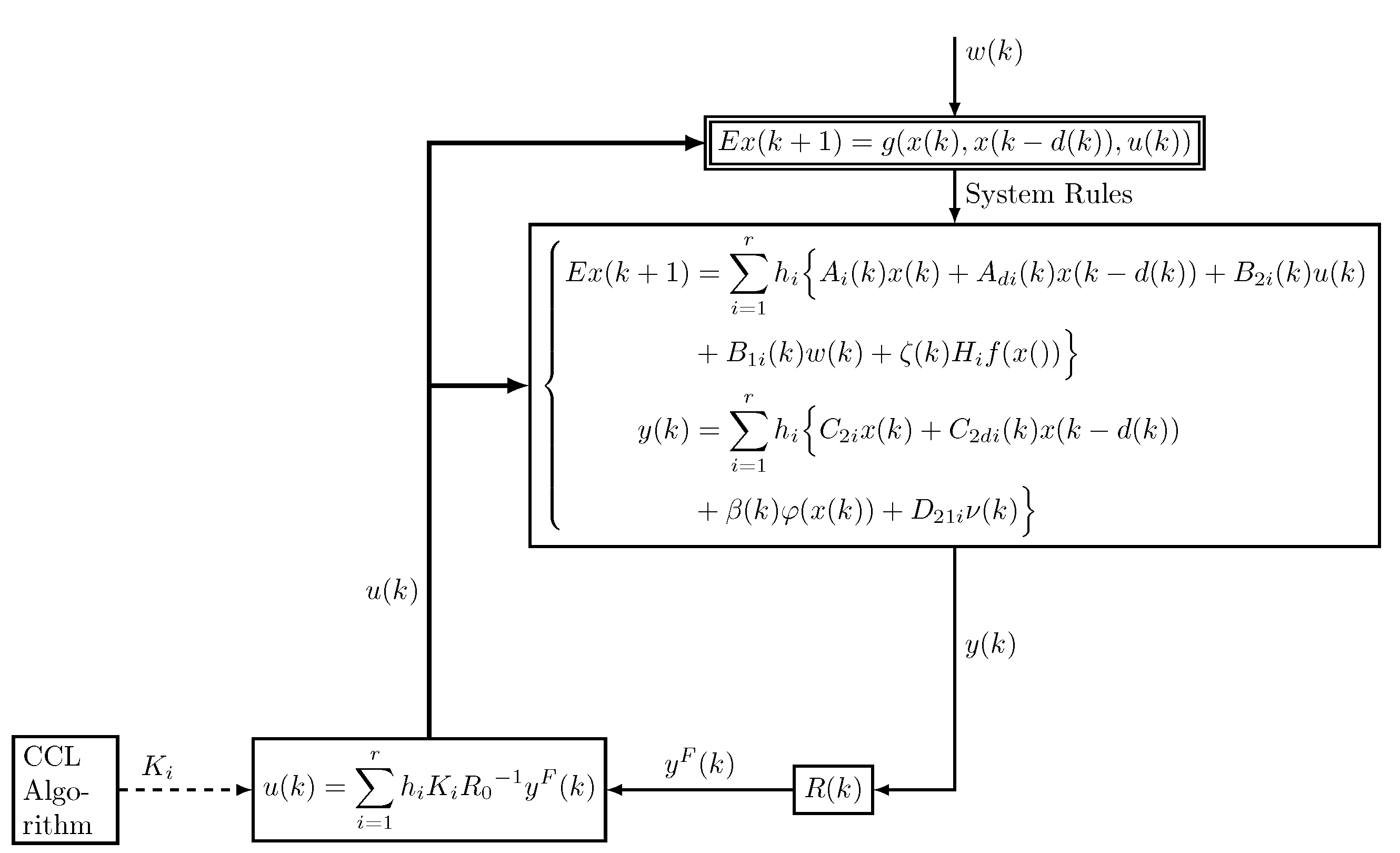
  • Design a new reliable SOF controller for a descriptor system subject to stochastic non-linearities and sensors failures;
  • Provide a simple method of the controller design based on introducing appropriate augmented closed-loop systems that decouple the output matrices and controller gain matrices;
  • Different from the works of [19,20], a new admissibility criterion with mixed H  /passive performance is derived for the closed-loop system, and with the help of the CCL algorithm, the effective reliable controllers gains are obtained..
The rest of the paper is organized as follows. In Section 2, some preliminaries are introduced. The admissibility analysis is conducted in Section 3. In Section 4, the design procedure of the fuzzy reliable static output feedback is presented, and a computational algorithm is given to characterize the design of the mixed H  /passive controller. Section 5 is dedicated to show the effectiveness of the theoretical results through three illustrative examples. A conclusion is given in Section 6.
Notations. The notations in this paper are quite standard, except where otherwise stated. The superscript T stands for matrix transposition; X R n denotes the n-dimensional Euclidean space, while X R n × m refers to the set of all n × m real matrices; X > 0 (respectively, X 0 ) means that the matrix X is real symmetric positive definite (respectively, positive semi-definite); l 2 [ 0 , ) is the space of square summable vectors; I and 0 represent the identity matrix and a zero matrix with appropriate dimensions, respectively; d i a g { } stands for a block-diagonal matrix; sym ( X ) stands for X + X T ; . denotes the Euclidean norm of a vector and its induced norm of a matrix; and E [ . ] stands for the mathematical expectation. In symmetric block matrices, we use a star * to represent a term that is induced by symmetry. Matrices, if their dimensions are not explicitly stated, are assumed to be compatible for algebraic operations. λ m a x ( ) means the largest eigenvalue of a matrix. To avoid clutter, in what follows, h i denotes h i ( θ ) , X θ represents the convex combination i = 1 r h i X i , and X θ θ will denote a convex combination of the form i = 1 r j = 1 r h i h j X i j .

2. Preliminaries

In this paper, the following TS fuzzy descriptor system is considered to describe the dynamic of a non-linear plant with time-varying delay:
E x ( k + 1 ) = i = 1 r h i ( θ ) A i ( k ) x ( k ) + A d i ( k ) x ( k d ( k ) ) + B 1 i w ( k ) + B i u ( k ) + ζ ( k ) H i f ( x ( k ) ) , z ( k ) = i = 1 r h i ( θ ) C 1 i x ( k ) + D 1 i w ( k ) , y ( k ) = i = 1 r h i ( θ ) C 2 i x ( k ) + C 2 d i ( k ) x ( k d ( k ) ) + β ( k ) φ ( x ( k ) ) + D 2 i ν ( k ) ) , x ( k ) = ϕ 0 ( l ) , l [ d M 0 ]
where x ( k ) R n is the state vector, u ( k ) R m is the control input, f ( x ( k ) ) and φ ( x ( k ) ) are randomly occurred non-linear functions, y ( k ) R p is the measured output, z ( k ) R n z is the controlled output, and w ( k ) R w and ν ( k ) R ν are the the exogenous disturbance signals, which are assumed to belong to l 2 [ 0 , ) . ϕ 0 ( l ) is a vector-valued function on [ d M 0 ] . Delay d ( k ) is time-varying and satisfies the following:
d m d ( k ) d M
where d m and d M are positive integers.
In this paper, we assume that matrix E R n × n may be singular and assume that rank ( E ) = q < n . A i ( k ) and A d i ( k ) are matrices with time-varying uncertainties, that is, the following:
A i ( k ) = A i + Δ A i ( k ) , A d i ( k ) = A d i + Δ A d i ( k )
Matrices A i , A d i , B 1 i , B i , H i , C 1 i , D 1 i , C 2 i , C 2 d i and D 2 i are known with appropriate dimensions. Δ A i ( k ) and Δ A d i ( k ) are unknown matrices representing time-varying parameter uncertainties.
In dealing with this study, the following assumptions are necessary for further development:
  • Δ A i ( k ) and Δ A d i ( k ) are assumed to satisfy the following admissible conditions:
    Δ A i ( k ) Δ A d i ( k ) = M i F ( k ) N i N d i , i = 1 , 2 , , r
    where M i , N i and N d i are known real constant matrices of appropriate dimensions, and F ( k ) R l is an unknown time-varying matrix function subject to F T ( k ) F ( k ) I k .
  • The non-linear functions f ( x ( k ) ) and φ ( x ( k ) ) are assumed to be continuous and satisfies the following conditions:
    f ( 0 ) = 0 , φ ( 0 ) = 0 [ f ( x ( k ) ) Ψ 1 x ( k ) ] T [ f ( x ( k ) ) Ω 1 x ( k ) ] 0 [ φ ( x ( k ) ) Ψ 2 x ( k ) ] T [ φ ( x ( k ) ) Ω 2 x ( k ) ] 0
    where Ψ 1 , Ω 1 , Ψ 2 and Ω 2 are real matrices with compatible dimensions.
As is well known, for many practical processes, such as networked control systems, the system output has a probabilistic aspect, due to the randomly missing data. In this study, we assume that the stochastic variables ζ ( k ) R and β ( k ) R are Bernoulli stochastic white sequences with the following distribution laws:
Prob { ζ ( k ) = 1 } = E { ζ ( k ) } = ζ ¯ , 0 ζ ¯ 1 , Prob { ζ ( k ) = 0 } = 1 ζ ¯ Prob { β ( k ) = 1 } = E { β ( k ) } = β ¯ , 0 β ¯ 1 , Prob { β ( k ) = 0 } = 1 β ¯
Obviously, for the stochastic variables ζ k and β k , we show the following:
E { ( ζ ( k ) ζ ¯ ) 2 } = ζ ¯ ( 1 ζ ¯ ) , E { ( β ( k ) β ¯ ) 2 } = β ¯ ( 1 β ¯ )
Remark 1.
  • In order to obtain a TS fuzzy model with a few rules, we can perform the sector non-linearity approach [17] for a restrictive number of non-linear terms included in the system under consideration. In addition, due to the environmental circumstances, such as random failures of the system components, sudden environment changes and unexpected change in the subsystem interconnections, etc., the processes are probably influenced by additive randomly occurred non-linear disturbances. Consequently, the term ζ k H i f ( x ( k ) ) in (1) involves both model uncertainties and random occurred non-linearities.
  • It is worth mentioning that sensors may not always produce ideal signals, due mainly to environmental constraints. The system’s output in (1) reflects tightly the reality; however, it turns out that the controller design is more difficult.
  • In this study, it is assumed that the non-linear functions belong to sectors. This description, suggested in [34], is more general, and includes the usual Lipschitz conditions as a special case.
Consider the following autonomous discrete-time descriptor system:
E x ( k + 1 ) = A x ( k ) + A d x ( k d ( k ) ) + B 1 w ( k ) z ( k ) = C x ( k ) + D w ( k )
Throughout the paper, the following definitions are adopted.
Definition 1
([1,35]). 
  • pair ( E , A ) is said to be regular if det ( z E A ) is not identically zero;
  • pair ( E , A ) is said to be causal, if it is regular and d e g d e t ( z E A ) = r a n k ( E ) ;
  • Pair ( E , A ) is said to be admissible, if it is regular, causal and stable;
Definition 2
([22]). For γ > 0 and 0 ϕ 1 , descriptor system (8) is said to be mean-square admissible with a mixed H  /passive performance γ, if under zero initial condition, the following inequality holds:
E k = 0 γ 1 ϕ z T ( k ) z ( k ) 2 γ ( 1 ϕ ) z T ( k ) w ( k ) < γ E k = 0 w T ( k ) w ( k )
for all 0 w ( k ) L 2 [ 0 , ) .
Remark 2.
Definition 2 includes both H  and strict passivity performances as special cases by choosing different values for ϕ.
  • If ϕ = 1 , inequality (9) reduces to an H  performance requirement.
  • If ϕ = 0 , inequality (9) corresponds to the passivity performance index.
We recall the following lemmas to be used in the proof of our main results.
Lemma 1
([36]). Given matrices M, N and P = P T of appropriate dimensions, then
P + M F ( k ) N + N T F T ( k ) M T < 0
for any F ( k ) satisfying F T ( k ) F ( k ) I , if and only if there exists a scalar ε > 0 such that the following holds:
P + ε M M T + ε 1 N T N < 0
Lemma 2
([37]). For any vectors ψ 1 , ψ 2 , matrices S, R and real scalars α 1 0 , α 2 0 , satisfying the following:
R S S T R 0 , α 1 + α 2 = 1 , ψ i = 0 i f α i = 0 ( i = 1 , 2 )
we have the following:
1 α 1 ψ 1 T R ψ 1 1 α 2 ψ 2 T R ψ 2 ψ 1 ψ 2 T R S S T R ψ 1 ψ 2

3. Admissibility Analysis

In this section, a new sufficient delay-dependent condition is established to deal with causality and stability for the nominal system of (1) (i.e., u ( k ) = 0 , w ( k ) = 0 and ζ ( k ) = 0 ). By invoking the delay bi-partitioning and improved reciprocally convex combination approaches, an LMI-based criterion is derived so that the descriptor system with delay is admissible.
Consider the following nominal compact presentation of (1).
E x ( k + 1 ) = A θ x ( k ) + A d θ x ( k d ( k ) )
As in [38], we denote
δ = d M + d m 2 + 1 2 min { ( 1 ) d M + d m , 0 } , τ M = d M δ , τ m = δ d m d r = d M d m
η ( k ) = x ( k + 1 ) x ( k ) , Γ ( k ) = col E x ( k ) , E η ( k ) , ξ ( k ) = col { x ( k ) , x ( k d m ) , x ( k d ( k ) ) , x ( k d M ) , x ( k δ ) , s = k d m k 1 E x ( s ) , s = k d M k d ( k ) 1 E x ( s ) , s = k d ( k ) k d m 1 E x ( s ) }
Γ 1 = col e 6 , E ( e 1 e 2 ) , Γ 21 = col e 7 , E ( e 3 e 4 ) , Γ 22 = col e 8 , E ( e 2 e 3 ) , Γ 2 = col Γ 21 , Γ 22 , Γ 3 = col E ( e 5 e 4 ) , E ( e 3 e 5 ) , E ( e 2 e 3 ) , Γ 4 = col E ( e 2 e 5 ) , E ( e 4 e 3 ) , E ( e 3 e 5 ) e i = 0 n , ( i 1 ) n I n 0 n , ( 8 i ) n , i = 1 , 2 , , 8 .
Theorem 1.
Given positive integers d m and d M . If there exist matrices P > 0 , Q 1 > 0 , Q 2 > 0 , Q 3 > 0 , Q 4 > 0 , Z 1 > 0 , Z 2 > 0 , W 1 > 0 , W 2 > 0 , R 1 , R 21 , R 22 , S 11 , S 12 , S 21 , S 22 , S, X and Y satisfying the following:
Φ 1 i = Φ 0 + Φ ( E , A i , A E i , A S i ) Γ 3 T W 1 Γ 3 < 0
Φ 2 i = Φ 0 + Φ ( E , A i , A E i , A S i ) Γ 4 T W 2 Γ 4 < 0
Z 1 > 0 , Z 2 > 0 , W 1 > 0 , W 2 > 0
where
Φ 0 = e 1 T Q 1 + Q 2 + Q 3 + ( d r + 1 ) Q 4 E T P E + d m E T R 1 E e 1 e 2 T Q 1 + d m E T R 1 E + d r E T R 22 E e 2 + e 3 T ( Q 4 + d r E T ( R 21 R 22 ) E ) e 3 e 4 T + Q 2 + d r E T R 21 E e 4 e 5 T Q 3 e 5 Γ 1 T Z 1 Γ 1 Γ 2 T Z 2 Γ 2
Φ ( E , A i , A E i , A S i ) = A i T P A i + A E i T τ m 2 W 1 + τ M 2 W 2 A E i + Y i T d m 2 Z 1 + d r 2 Z 2 Y i + sym e 1 T S R 0 T A S i
Z 1 = Z 1 11 Z 1 12 * Z 1 22 Z 2 = Z 2 11 Z 2 12 * Z 2 22 Z 1 = Z 1 11 Z 1 12 + R 1 * Z 1 22 + R 1 Z 21 = Z 2 11 Z 2 12 + R 21 * Z 2 22 + R 21 Z 22 = Z 2 11 Z 2 12 + R 22 * Z 2 22 + R 22 W 1 = W 2 0 0 * W 1 X * * W 1 W 2 = W 1 0 0 * W 2 Y * * W 2 Z 2 = Z 21 S * Z 22 S = S 11 S 12 S 21 S 22 , A i = A i e 1 + A d i e 3 , A E i = ( A i E ) e 1 + A d i e 3 , A S i = A i e 1 + A d i e 3 , Y i = col E e 1 , A E i
then, system (11) is admissible. R 0 R n × n r is any matrix with full column rank satisfying E T R 0 = 0 .
Proof. 
First, we prove the regularity and causality properties of the system.
Since rank ( E ) = q < n , there always exist two non-singular matrices M ^ and N ^ R n × n such that the following holds:
E ^ = M ^ E N ^ = I q 0 0 0
Then, R 0 can be characterized as the following: R 0 = M ^ T 0 R ^ 0 , where R ^ 0 R ( n q ) × ( n q ) is any non-singular matrix. We define also the following:
A ^ i = M ^ A i N ^ = A ^ 11 i A ^ 12 i A ^ 21 i A ^ 22 i , S ^ = N ^ T S = S ^ 11 S ^ 21 , A ^ d i = M ^ A d i N ^ = A ^ d 11 i A ^ d 12 i A ^ d 21 i A ^ d 22 i .
From (15) and (16) the following inequality holds:
sym ( S R 0 T A i ) + d m 2 sym ( E T Z 1 12 ( A i E ) ) + d r 2 sym ( E T Z 2 12 ( A i E ) ) + d m E T R 1 E E T ( Z 1 22 + R 1 ) E + d m 2 E T Z 1 11 E + d r 2 E T Z 2 11 E E T P E < 0
Since h i ( θ ) 0 and i = 1 r h i ( θ ) = 1 , it yields the following:
sym ( S R 0 T A θ ) + d m 2 sym ( E T Z 1 12 ( A θ E ) ) + d r 2 sym ( E T Z 2 12 ( A θ E ) ) + d m E T R 1 E E T ( Z 1 22 + R 1 ) E + d m 2 E T Z 1 11 E + d r 2 E T Z 2 11 E E T P E < 0
Pre- and post-multiplying (24) by M ^ T and M ^ , respectively, and then using expressions (21) and (22) gives the following:
s y m ( S ^ 21 R ^ 0 T A ^ 22 θ ) < 0
and A ^ 22 θ is, thus, non-singular. For the stability analysis of system (11), we construct the following Lyapunov–Krasovskii functional:
V ( k ) = V 1 ( k ) + V 3 ( k ) + V 3 ( k ) + V 4 ( k ) V 1 ( k ) = x T ( k ) E T P E x ( k ) V 2 ( k ) = s = k d m k 1 x T ( s ) Q 1 x ( s ) + s = k d M k 1 x T ( s ) Q 2 x ( s ) + s = k δ k 1 x T ( s ) Q 3 x ( s ) + θ = d M d m s = k + θ k 1 x T ( s ) Q 4 x ( s ) V 3 ( k ) = τ m θ = δ d m 1 s = k + θ k 1 η T ( s ) E T W 1 E η ( s ) + τ M θ = d M δ 1 s = k + θ k 1 η T ( s ) E T W 2 E η ( s ) V 4 ( k ) = d m θ = d m 1 s = k + θ k 1 Γ T ( s ) Z 1 Γ ( s ) + d r θ = d M d m 1 s = k + θ k 1 Γ T ( s ) Z 2 Γ ( s )
Calculating the difference of V ( k ) along the system trajectories, one obtains the following:
Δ V 1 ( k ) = A θ x ( k ) + A d θ x ( k d ( k ) ) T P A θ x ( k ) + A d θ x ( k d ( k ) ) E T P E = ξ T ( k ) A θ T P A θ e 1 T E T P E e 1 ξ ( k ) Δ V 2 ( k ) ξ T ( k ) ( e 1 T Q 1 + Q 2 + Q 3 + ( d r + 1 ) Q 4 e 1 e 2 T Q 1 e 2 e 4 T Q 2 e 4 e 5 T Q 3 e 5 e 3 T Q 4 e 3 ) ξ ( k ) Δ V 3 ( k ) = ξ T ( k ) A E θ T τ m 2 W 1 + τ M 2 W 2 A E θ ξ ( k ) τ m s = k δ k d m 1 η T ( s ) E T W 1 E η ( s ) τ M s = k d M k δ 1 η T ( s ) E T W 2 E η ( s ) Δ V 4 ( k ) = Γ T ( k ) d m 2 Z 1 + d r 2 Z 2 Γ ( k ) d m s = k d m k 1 Γ T ( s ) Z 1 Γ ( s ) d r s = k d M k d ( k ) 1 Γ T ( s ) Z 2 Γ ( s ) d r s = k d ( k ) k d m 1 Γ T ( s ) Z 2 Γ ( s )
For any symmetrical matrix R 1 , one can verify the following:
s = k d m k 1 x T ( s + 1 ) E T R 1 E x ( s + 1 ) x T ( s ) E T R 1 E x ( s ) = s = k d m k 1 η T ( s ) E T R 1 E η ( s ) + 2 x T ( s ) E T R 1 E η ( s ) = s = k d m k 1 Γ T ( s ) 0 R 1 R 1 T R 1 Γ ( s ) = x T ( k ) E T R 1 E x ( k ) x T ( k d m ) E T R 1 E x ( k d m )
From Equation (28), the following null equation holds:
x T ( k ) E T R 1 E x ( k ) x T ( k d m ) E T R 1 E x ( k d m ) s = k d m k 1 Γ T ( s ) 0 R 1 R 1 T R 1 Γ ( s ) = 0
Then, by adding the previous zero-value equation and using the Jensen inequality, algebraic manipulation yields the following:
d m s = k d m k 1 Γ T ( s ) Z 1 Γ ( s ) = ξ T ( k ) ( d m e 1 T E T R 1 E e 1 d m e 2 T E T R 1 E e 2 ) ξ ( k ) d m s = k d m k 1 Γ T ( s ) Z 1 Γ ( s ) ξ T ( k ) d m e 1 T E T R 1 E e 1 d m e 2 T E T R 1 E e 2 ξ ( k ) Γ 1 T Z 1 Γ 1
Following the same procedure as above, the following inequalities can be established:
d r s = k d M k d ( k ) 1 Γ T ( s ) Z 2 Γ ( s ) ξ T ( k ) d r e 3 T E T R 21 E e 3 d r e 4 T E T R 21 E e 4 ξ ( k ) d r d M d ( k ) Γ 21 T Z 21 Γ 21 d r s = k d ( k ) k d m 1 Γ T ( s ) Z 2 Γ ( s ) ξ T ( k ) d r e 2 T E T R 22 E e 2 d r e 3 T E T R 22 E e 3 ξ ( k ) d r d ( k ) d m Γ 22 T Z 22 Γ 22
According to Lemma 2, one obtains the following:
d r s = k d M k d m 1 Γ T ( s ) Z 2 Γ ( s ) ξ T ( k ) ( d r e 2 T E T R 22 E e 2 + d r e 3 T E T ( R 21 R 22 ) E e 3 d r e 4 T E T R 21 E e 4 ) ξ ( k ) Γ 2 T Z 2 Γ 2
On the other hand, when d m d ( k ) δ , we derive the following:
τ m s = k δ k d m 1 η T ( s ) E T W 1 E η ( s ) = τ m s = k δ k d ( k ) 1 η T ( s ) E T W 1 E η ( s ) τ m s = k d ( k ) k d m 1 η T ( s ) E T W 1 E η ( s ) τ m δ d ( k ) ξ T ( k ) ( e 3 e 5 ) T E T W 1 E ( e 3 e 5 ) ξ ( k ) τ m d ( k ) d m ξ T ( k ) ( e 2 e 3 ) T E T W 1 E ( e 2 e 3 ) ξ ( k )
and
τ M s = k d M k δ 1 η T ( s ) E T W 2 E η ( s ) ξ T ( k ) ( e 5 e 4 ) T E T W 2 E ( e 5 e 4 ) ξ ( k )
Then, the following condition holds using Lemma 2:
τ m s = k δ k d m 1 η T ( s ) E T W 1 E η ( s ) τ M s = k d M k δ 1 η T ( s ) E T W 2 E η ( s ) Γ 3 T W 1 Γ 3
Note that E T R 0 = 0 , for any matrix S with appropriate dimensions yields the following:
2 x ( k ) S R 0 T E x ( k + 1 ) = 2 ξ T ( k ) e 1 T S R 0 T A S θ = 0
Combining (27)–(36), we have the following:
Δ V ( k ) ξ T ( k ) Φ 1 θ ξ ( k )
When δ d ( k ) d M , by proceeding as before, it is readily seen that the following condition is verified:
τ m s = k δ k d m 1 η T ( s ) E T W 1 E η ( s ) τ M s = k d M k δ 1 η T ( s ) E T W 2 E η ( s ) Γ 4 T W 2 Γ 4
and then, we obtain the following:
Δ V ( k ) ξ T ( k ) Φ 2 θ ξ ( k )
Hence, under the conditions of Theorem 1, we can deduce from (37) and (39) the following:
V ( k + 1 ) V ( k ) α ξ ( k ) 2 , α = max λ m a x Φ 1 i , λ m a x Φ 2 i
From (40), one can obtain the following:
V ( k + 1 ) V ( 0 ) α l = 0 k ξ ( l ) 2
and therefore, we obtain the following:
l = 0 k ξ ( l ) 2 1 α V ( 0 ) <
which implies lim k ξ ( k ) = 0 . Thus, system (11) is stable. This concludes the proof.    □
Remark 3.
We would like to stress that in order to obtain less conservative stability conditions for discrete-time singular systems, the authors in [10] proposed a new Lyapunov functional with triple sum, and the reciprocally convex combination approach is extended to bound the double summable term. The authors in [11] developed a new summation inequality as a less conservative extension of the Jensen inequality. However, the key merit of the obtained less conservative criterion lies in the application of the delay partitioning method combined with the improved reciprocally convex combination approach.

4. Reliable SOF Controller Design

In this section, we shall focus on the reliable output feedback control design problem whose purpose is to design a reliable mixed H  /passive controller for system (1) via a fuzzy static output controller. Assume that the sensors suffer from failures. The following model of failure is adopted in this paper to describe the measured signal sent from the sensors as follows:
y F ( k ) = R ( k ) y ( k )
where R ( k ) is the sensor fault matrix defined as follows:
R ( k ) = diag r 1 ( k ) , r 2 ( k ) , , r p ( k ) r ̲ s r s ( k ) r ¯ s , s = 1 , 2 , p
where r s ( k ) is the degradation level of the ’s’th sensor.
Let the following hold:
Q = diag q 1 , q 2 , , q p , q s = r ¯ s r ̲ s r ̲ s + r ¯ s , R 0 = diag r 01 , r 02 , , r 0 p , r 0 s = r ̲ s + r ¯ s 2 , ( s = 1 , 2 , p ) G ( k ) = diag g 1 ( k ) , g 2 ( k ) , , g p ( k ) , g s ( k ) = r s ( k ) r 0 s r 0 s
Matrix R ( k ) can be rewritten as the following:
R ( k ) = R 0 ( I + G ( k ) )
It can be verified that the following holds:
G ( k ) Q
The problem of mixed H  /passive reliable SOF control could be phrased as follows: given the fuzzy system in (1), determine a reliable SOF control law as follows:
u ( k ) = i = 1 r h i K i R 0 1 y F ( k ) = K θ R 0 1 y F ( k )
such that, for all admissible sensor failures and exogenous disturbances, the following requirements are ensured:
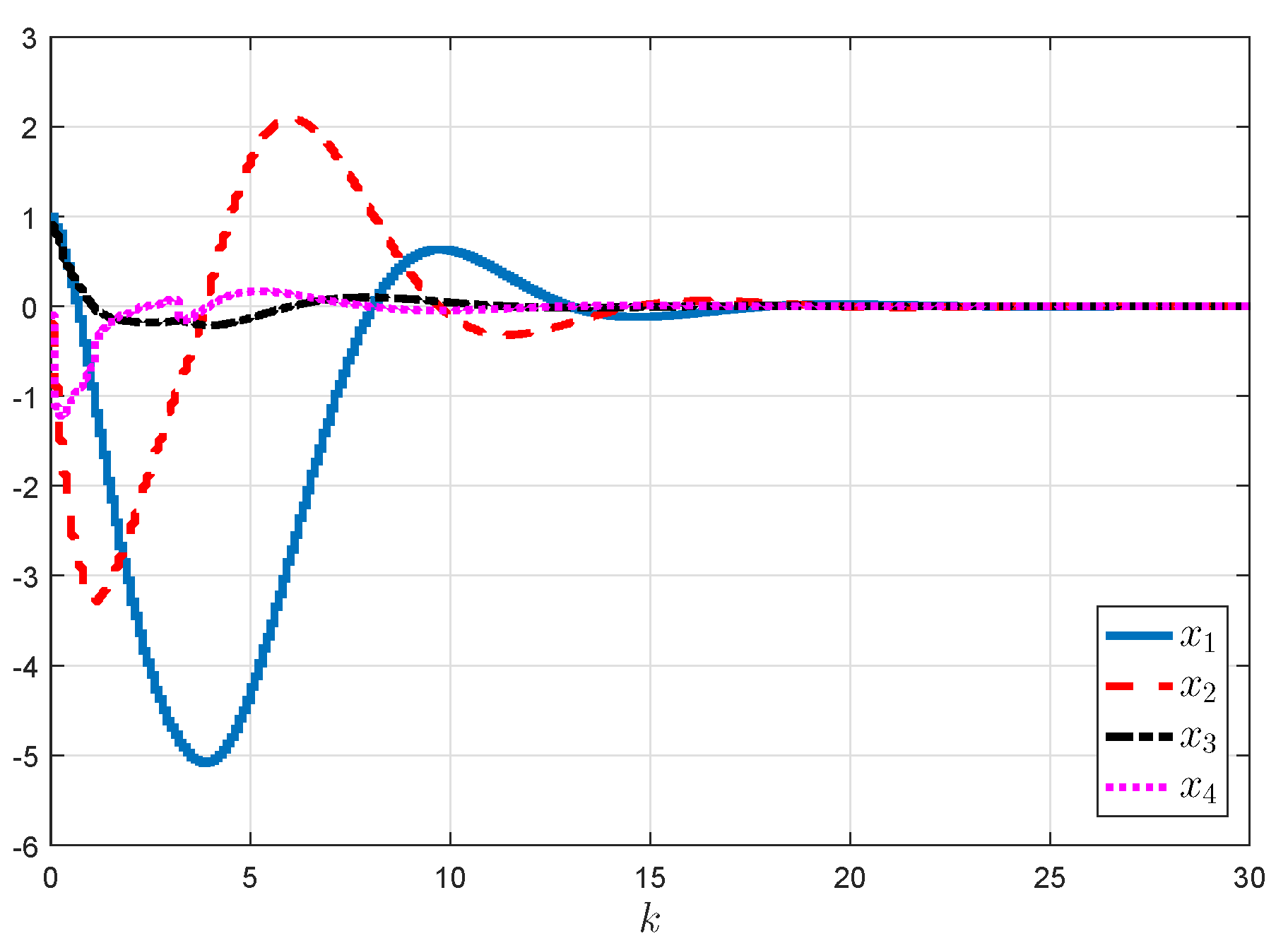
  • The resulting closed-loop system is robustly mean-square admissible,
  • Under zero-initial condition, the mixed H  /passive performance is satisfied in the sense of Definition 2.
K i is compatible with the dimensional control gain.
Since the system output contains probabilistic missing data and noise, the design of the SOF controller using the standard approach is made difficult, even impossible. To overcome this problem, we propose the transformation that considers y ( k ) as a state component. The closed-loop system has the following structure:
( Σ c ) : E ¯ x ¯ ( k + 1 ) = A ¯ θ θ ( k ) x ¯ ( k ) + A ¯ d θ ( k ) x ¯ ( k d ( k ) ) + B ¯ 1 θ w ¯ ( k ) + Π ¯ H ¯ θ f ¯ + ( Π ( k ) Π ¯ ) H ¯ θ f ¯ , z ( k ) = C ¯ 1 θ x ¯ ( k ) + D ¯ 1 θ w ¯ ( k ) ,
where x ¯ ( k ) = x T ( k ) y T ( k ) T , w ¯ ( k ) = w T ( k ) ν T ( k ) T ,     f ¯ = f T ( x ( k ) ) φ T ( x ( k ) ) T , A ¯ θ θ ( k ) = A ¯ θ θ + M ¯ θ F ( k ) N ¯ θ , A ¯ d θ ( k ) = A ¯ d θ + M ¯ θ F ( k ) N ¯ d θ ,
E ¯ = E 0 0 0 , A ¯ θ θ = A θ B θ K θ ( k ) C 2 θ I , A ¯ d θ = A d θ 0 C 2 d θ 0 , B ¯ 1 θ = B 1 θ 0 0 D 2 θ , C ¯ 1 θ = C 1 θ 0 , D ¯ 1 θ = D 1 θ 0 , H ¯ θ = H θ 0 0 I , M ¯ θ = M θ T 0 T , N ¯ θ = N θ 0 , N ¯ d θ = N d θ 0 , Π ( k ) = ζ ( k ) 0 0 β ( k ) ,
Easily, we can verify the following: A ¯ θ θ = A ¯ θ 0 + B ¯ θ K ¯ θ ( I + G ( k ) ) . where
A ¯ θ 0 = A θ 0 C 2 θ I , B ¯ θ = B θ 0 , K ¯ θ = 0 K θ ,

4.1. Mixed H  /Passive Analysis

Our goal here is to establish a tractable condition satisfying system (49) to be mean-square admissible with a mixed weighted H  /passive performance index γ .
Theorem 2.
Given positive integers d m , d M and a positive scalar 0 ϕ 1 . The closed-loop system ( Σ c ) without uncertainties is admissible in the mean square for w ( k ) = 0 and satisfies the mixed weighted H  /passive performance index (9) under zero initial condition for any non-zero w l 2 [ 0 , ) , if there exist a positive scalar τ and matrices P ¯ > 0 , Q ¯ 1 > 0 , Q ¯ 2 > 0 , Q ¯ 3 > 0 , Q ¯ 4 > 0 , W ¯ 1 > 0 , W ¯ 2 > 0 , V ¯ > 0 , S ¯ , X ¯ and Y ¯ satisfying the following:
Φ ¯ 1 i j A ¯ i j , A ¯ E i j , A ¯ S i j 0 < 0
Φ ¯ 2 i j A ¯ i j , A ¯ E i j , A ¯ S i j 0 < 0
where
Φ ¯ l i j A ¯ i j , A ¯ E i j , A ¯ S i j 0 = Φ ¯ 11 l i j ϕ C ¯ i T A ¯ i j T τ m A ¯ E i j T τ M A ¯ E i j T B ¯ S i K ¯ j T K ¯ j 0 T * γ I 0 0 0 0 0 * * P ¯ 1 0 0 0 0 * * * W ¯ 1 1 0 0 0 * * * * W ¯ 2 1 0 0 * * * * * V ¯ 1 0 * * * * * * V ¯ ,
l = 1 , 2
Φ ¯ 11 l i j = Φ ¯ 0 Γ 2 + l T W l Γ 2 + l + sym e 1 T S R 0 T A ¯ S i j 0 + Φ ¯ c i Φ ¯ 0 = e 1 T Q ¯ 1 + Q ¯ 2 + Q ¯ 3 + ( d r + 1 ) Q ¯ 4 E T P E τ Ψ ^ e 1 e 2 T Q ¯ 1 e 2 e 3 T Q ¯ 4 e 3 e 4 T Q ¯ 2 e 4 τ sym e 1 T Ω ^ e 6 τ e 6 T e 6 A ¯ i j = A ¯ i j e 1 + A ¯ d i e 3 + Π ¯ + Π ¯ ( 1 Π ¯ ) H ¯ i e 6 + B ¯ 1 i e 7 , A ¯ E i j = ( A ¯ i j E ¯ ) e 1 + A ¯ d i e 3 + Π ¯ + Π ¯ ( 1 Π ¯ ) H ¯ i e 6 + B ¯ 1 i e 7 , A ¯ S i j 0 = A ¯ i j 0 e 1 + A ¯ d i e 3 + Π ¯ H ¯ i e 6 + B ¯ 1 i e 7 , A ¯ i j 0 = A ¯ i 0 + B ¯ i K ¯ i 0 C ¯ i = C ¯ 1 i e 1 + D ¯ 1 i e 7 K ¯ i = K ¯ i e 1 , K ¯ i 0 = K ¯ i 0 e 1 , B ¯ S i = e 1 T S R 0 T B ¯ i Ψ ^ = Ψ 1 T Ω 1 + Ω 1 T Ψ 1 2 , Ω ^ = Ψ 1 T + Ω 1 T 2
R ¯ 0 is any matrix with full column rank satisfying E ¯ T R ¯ 0 = 0 and K i 0 are given matrices such that A i + B 2 i K i 0 C 2 i is Hurwitz.
Proof. 
To improve the computational efficiency, we select the Lyapunov–Krasovskii functional (26) without the V 4 ( k ) term.
Calculating the difference of V ( k ) along the system (49) and taking the mathematical expectation, we have the following:
E Δ V 1 ( k ) = E { A ¯ θ θ ( k ) x ¯ ( k ) + A ¯ d θ ( k ) x ¯ ( k d ( k ) ) + B ¯ 1 θ w ¯ ( k ) + Π ¯ H ¯ θ f ¯ + ( Π ( k ) Π ¯ ) H ¯ θ f ¯ T P ¯ A ¯ θ θ ( k ) x ¯ ( k ) + A ¯ d θ ( k ) x ¯ ( k d ( k ) ) + B ¯ 1 θ w ¯ ( k ) + Π ¯ H ¯ θ f ¯ + ( Π ( k ) Π ¯ ) H ¯ θ f ¯ E ¯ T P ¯ E ¯ } = E ψ T ( k ) A ¯ θ θ T P ¯ A ¯ θ θ e 1 T E ¯ T P ¯ E ¯ e 1 ψ ( k ) E Δ V 2 ( k ) E { ψ T ( k ) ( e 1 T Q ¯ 1 + Q ¯ 2 + Q ¯ 3 + ( d r + 1 ) Q ¯ 4 e 1 e 2 T Q ¯ 1 e 2 e 4 T Q ¯ 2 e 4 e 5 T Q ¯ 3 e 5 e 3 T Q ¯ 4 e 3 ) ψ ( k ) } E Δ V 3 ( k ) = E { ψ T ( k ) A ¯ E θ θ T τ m 2 W ¯ 1 + τ M 2 W ¯ 2 A ¯ E θ θ ψ ( k ) τ m s = k δ k d m 1 η T ( s ) E ¯ T W ¯ 1 E ¯ η ( s ) τ M s = k d M k δ 1 η T ( s ) E ¯ T W ¯ 2 E ¯ η ( s ) }
Note that E ¯ T R ¯ 0 = 0 , for any matrix S ¯ with appropriate dimensions yields the following:
E 2 x ¯ ( k ) S ¯ R ¯ 0 T E x ¯ ( k + 1 ) = E { 2 ψ T ( k ) e 1 T S ¯ R ¯ 0 T A ¯ S θ θ } = 0
Furthermore, from assumption 2 the following inequality holds for any τ > 0 as follows:
x ¯ ( k ) f ¯ T τ Ψ ^ τ Ω ^ * τ I x ¯ ( k ) f ¯ 0
Combining (57)–(59), it follows for d m d ( k ) δ that we have the following:
E Δ V ( k ) E { ψ T ( k ) Φ ¯ 0 Γ 3 T W 1 Γ 3 + Φ ¯ ( E ¯ , A ¯ θ θ , A ¯ E θ θ , A ¯ S θ θ ) ψ ( k ) }
When δ d ( k ) d M , we derive the following:
E Δ V ( k ) E { ψ T ( k ) Φ ¯ 0 Γ 4 T W 2 Γ 4 + Φ ¯ ( E ¯ , A ¯ θ θ , A ¯ E θ θ , A ¯ S θ θ ) ψ ( k ) }
where
Φ ¯ ( E ¯ , A ¯ θ θ , A ¯ E θ θ , A ¯ S θ θ ) = A ¯ θ θ T P ¯ A ¯ θ θ + A ¯ E θ θ T τ m 2 W ¯ 1 + τ M 2 W ¯ 2 A ¯ E θ θ + sym e 1 T S ¯ R ¯ 0 T A ¯ S θ θ ψ ( k ) = col x ¯ ( k ) , x ¯ ( k d m ) , x ¯ ( k d ( k ) ) , x ¯ ( k d M ) , x ¯ ( k δ ) , f ¯ ( x ( k ) ) , w ¯ ( k )
Note that sym e 1 T S ¯ R ¯ 0 T A ¯ S i j = sym e 1 T S ¯ R ¯ 0 T A ¯ S i 0 + B ¯ S i K ¯ j . For an appropriate dimensional matrix V ¯ > 0 , the following inequality holds:
B ¯ S i T V ¯ ( K ¯ j K ¯ j 0 ) T V ¯ 1 B ¯ S i T V ¯ ( K ¯ j K ¯ j 0 ) 0
Equivalently, we obtain the following:
sym B ¯ S i K ¯ j B ¯ S i V ¯ 1 B ¯ S i T + ( K ¯ j K ¯ j 0 ) T V ¯ ( K ¯ j K ¯ j 0 ) + sym B ¯ S i K ¯ j 0
Then
sym e 1 T S R 0 T A ¯ S i j sym e 1 T S R 0 T A ¯ S i j 0 + B ¯ S i V ¯ 1 B ¯ S i T + ( K ¯ j K ¯ j 0 ) T V ¯ ( K ¯ j K ¯ j 0 )
Furthermore, by the Schur complement, we can deduce from (52)–(53) that the following holds:
Φ ¯ 0 Γ 2 + l T W l Γ 2 + l + Φ ¯ ( E , A ¯ θ θ , A ¯ E θ θ , A ¯ S θ θ ) < 0 , l = 1 , 2 .
Thus, system (49) with w ¯ ( k ) = 0 is admissible in the mean square.
To further investigate the mixed H  /passive performance of the system in (11), we introduce the following performance index:
J z w = E k = 0 γ 1 ϕ z T ( k ) z ( k ) 2 γ ( 1 ϕ ) z T ( k ) w ¯ ( k ) γ w ¯ T ( k ) ( k ) w ¯ ( k )
under zero initial condition, we have the following:
J z w = E k = 0 Δ V ( k ) + γ 1 ϕ z T ( k ) z ( k ) 2 γ ( 1 ϕ ) z T ( k ) w ¯ ( k ) γ w ¯ T ( k ) ( k ) w ¯ ( k ) E V ( ) E k = 0 Δ V ( k ) + γ 1 ϕ z T ( k ) z ( k ) 2 γ ( 1 ϕ ) z T ( k ) w ¯ ( k ) γ w ¯ T ( k ) ( k ) w ¯ ( k )
Let the following hold: Φ ¯ c θ = 2 γ ( 1 ϕ ) sym C θ T e 7 γ e 7 T e 7 . From (52) to (53), the following can be deduced:
E Δ V ( k ) + γ 1 ϕ z T ( k ) z ( k ) 2 γ ( 1 ϕ ) z T ( k ) w ¯ ( k ) γ w ¯ T ( k ) w ¯ ( k ) = E { ψ T ( k ) Φ ¯ 0 Γ l + 2 T W l Γ l + 2 + Φ ¯ ( E , A ¯ θ θ , A ¯ E θ θ , A ¯ S θ θ ) + Φ ¯ c θ + γ 1 ϕ C θ T C θ ψ ( k ) } < 0 , l = 1 , 2
Thus, system (49) is with a mixed weighted H  /passive performance index γ in the sense of Definition 2. This completes the proof.    □
Remark 4.
To reduce the conservativeness of the proposed conditions, matrix K i 0 is introduced such that A i + B 2 i K i 0 C 2 i is Hurwitz.

4.2. Reliable Controller Synthesis

Theorem 3.
Given positive integers d m , d M and a positive scalar 0 ϕ 1 . The closed-loop system ( Σ c ) is admissible in the mean square for w ( k ) = 0 and satisfies the mixed weighted H  /passive performance index (9) under zero initial condition for any non-zero w l 2 [ 0 , ) , if there exist positive scalars τ, ε i , κ i and matrices P ¯ > 0 , P ^ > 0 , Q ¯ 1 > 0 , Q ¯ 2 > 0 , Q ¯ 3 > 0 , Q ¯ 4 > 0 , W ¯ 1 > 0 , W ^ 1 > 0 , W ¯ 2 > 0 , W ^ 2 > 0 , V ¯ > 0 , V ^ > 0 , Z ¯ > 0 , S ¯ , X ¯ and Y ¯ satisfying the following:
Φ ^ 1 i i < 0 , i = 1 , , r
Φ ^ 2 i i < 0 , i = 1 , , r
2 r 1 Φ ^ 1 i i + Φ ^ 1 i j + Φ ^ 1 j i < 0 , i j = 1 , , r
2 r 1 Φ ^ 2 i i + Φ ^ 2 i j + Φ ^ 2 j i < 0 , i j = 1 , , r
P ¯ P ^ = I , W ¯ 1 W ^ 1 = I , W ¯ 2 W ^ 2 = I , V ¯ V ^ = I
where
Φ ^ l i j = Φ ^ 11 l i j ε i N ¯ i T M ¯ i B ¯ i Z ¯ Q T K ¯ j T * ε i I 0 0 0 * * ε i I 0 0 * * * Z ¯ 0 * * * * Z ¯ Φ ^ 11 l i j = Φ ¯ 11 l i j ϕ C ¯ i T A ¯ i j T τ m A ¯ E i j T τ M A ¯ E i j T B ¯ S i K ¯ j T K ¯ j 0 T * γ I 0 0 0 0 0 * * P ^ 0 0 0 0 * * * W ^ 1 0 0 0 * * * * W ^ 2 0 0 * * * * * V ¯ 0 * * * * * * V ^ M ¯ i = M ¯ i T 0 0 τ m M ¯ i T τ M M ¯ i T M ¯ i T 0 0 T , N ¯ i = N ¯ i 0 0 0 0 0 0 0 B ¯ i = 0 0 0 B ¯ i T τ m B ¯ i T τ M B ¯ i T 0 I T , K ¯ i = K ¯ i 0 0 0 0 0 0 0 N ¯ i = N ¯ i e 1 + N ¯ d i e 3 , M ¯ i = e 1 T S ¯ R ¯ 0 T M ¯ i
Proof. 
By substituting A ¯ i j ( k ) and A ¯ d i ( k ) in (52) and (53), the following conditions holds:
Φ ¯ l i j ( k ) = Φ ¯ l i j + sym M ¯ i F ( k ) N ¯ i + sym B ¯ i K ¯ j ( k ) < 0
Using Lemma 1, Equation (76) is equivalent to the following:
Φ ¯ l i j ε i N ¯ i T M ¯ i * ε i I 0 * * ε i I + sym B ¯ i T K ¯ j R ( k ) < 0
where R ( k ) = diag R ¯ ( k ) , I , I , I , I , I , I , I and R ¯ ( k ) = diag I , R ( k ) . For any appropriate matrix Z ¯ > 0 yields the following:
Z ¯ B ¯ i K ¯ j R ( k ) T Z ¯ 1 Z ¯ B ¯ i K ¯ j R ( k ) 0
Using the fact that G ( k ) Q , we obtain the following:
sym B ¯ i T K ¯ j R ( k ) B ¯ i T Z ¯ Z ¯ 1 Z ¯ B ¯ i + Q T K ¯ j T Z ¯ 1 K ¯ j Q
then Φ ^ l i j < 0 holds using Schur complement.
Based on the parametrized linear matrix inequality (PLMI) proposed in [39], relaxed conditions are obtained in (70)–(73). This completes the proof.    □
Remark 5.
Due to equality constraints (74), conditions (70)–(73) are not in strict LMI form which cannot be solved directly using the standard LMI procedures. For applying the LMI technique, we can formulate this non-convex feasibility problem into a sequential optimization problem subject to LMIs constraints.
Based on the cone complementarity linearization (CCL) technique [40], we propose the following minimization problem involving LMI conditions instead of the original non-convex condition (74).
m i n Tr ( P ¯ P ^ + W ¯ 1 W ^ 1 + W ¯ 2 W ^ 2 + V ¯ V ^ ) , subject to
( 70 ) ( 73 ) P ¯ I I P ^ 0 W ¯ 1 I I W ^ 1 0 W ¯ 2 I I W ^ 2 0 V ¯ I I V ^ 0
If the solution of the above minimization problem is 3 n ¯ + m , ( n ¯ = n + p ), that is,
m i n Tr ( P ¯ P ^ + W ¯ 1 W ^ 1 + W ¯ 2 W ^ 2 + V ¯ V ^ ) = 3 n ¯ + m
then, the conditions in Theorem 2 are solvable. In order to find a feasible solution of the above minimization problem, we suggest the following Algorithm 1:
Algorithm 1: Find a feasible solution of the above minimisation problem
step 1
Find a feasible set P ¯ ( 0 ) , P ^ ( 0 ) , W ¯ 1 ( 0 ) , W ^ 1 ( 0 ) , W ¯ 2 ( 0 ) , W ^ 2 ( 0 ) , V ¯ ( 0 ) , V ^ ( 0 )
satisfying (70)–(73). Set k = 0 .
step 2
Solve the following optimization problem:
m i n Tr ( P ^ ( k ) P ¯ + P ¯ ( k ) P ^ + Z ^ 1 ( k ) W ¯ 1 + W ¯ 1 ( k ) W ^ 1 + W ^ 2 ( k ) W ¯ 2 + W ¯ 2 ( k ) W ^ 2 + V ^ ( k ) V ¯ + V ¯ ( k ) V ^ )
subject to (81).
step 3
if | Tr ( P ¯ P ^ + W ¯ 1 W ^ 1 + W ¯ 2 W ^ 2 + V ¯ V ^ ( 3 n ¯ + m ) | < ϵ ,
for a sufficiently small scalar ϵ > 0 , the solution K i , i = 1 , 2 , , r ,
is the controller gains.
STOP .
else
Set k = k + 1 , set ( P ¯ ( k ) , P ^ ( k ) , W ¯ 1 ( k ) , W ^ 1 ( k ) , W ¯ 2 ( k ) , W ^ 2 ( k ) , V ¯ ( k ) , V ^ ( k ) )
= ( P ¯ , P ^ , W ¯ 1 , W ^ 1 , W ¯ 2 , W ^ 2 , V ¯ , V ^ ), and go to Step 2.
step 4
If k > N , where N is the maximum number of iterations allowed, EXIT.
Our method fails to find feasible gains.
Remark 6.
The flowchart displayed in Figure 1 provides a clear description of the proposed design procedure. Moreover, this procedure can be also applied for a standard system with E = I .
Remark 7.
As mentioned in Remark 1, the non-linear functions are assumed that belong to sectors. For more general cases, if the non-linear perturbations satisfy the so-called one-sided Lipschitz constraint, the proposed approach cannot be applied. This interesting issue should be considered in future studies [27].

5. Numerical Examples

In this section, three numerical examples are provided to validate the effectiveness and advantage of the developed results.
Example 1.
In this example, we demonstrate the advantage of the proposed admissibility method over some existing ones. Consider the following discrete-time singular system with delay.
E = 1 0 0 0 , A = 0.8 0 0.05 0.9 , A = 0.1 0 0.2 0.1
For various values of d m , Table 1 shows the admissible maximum values of d M that guarantees the discrete singular time-delay system to be admissible by applying the result suggested in this study and the methods proposed in [5,6,7,8,9,10,11]. From the table, we observe that the admissibility criterion in Theorem 1 is less conservative than those proposed in [5,6,7,8,9,10,11].
Example 2.
Referring to [41], we consider the following modified truck-trailer mapping system with stochastic disturbances:
x 1 ( k + 1 ) = c 1 v t L t 0 x 1 ( k ) + ( 1 c ) 1 v t L t 0 x 1 ( k d ( k ) ) + v t l t 0 u ( k ) + 0.1 w ( k ) x 2 ( k + 1 ) = c v t L t 0 x 1 ( k ) + ( 1 c ) v t L t 0 x 1 ( k d ( k ) ) + x 2 ( k ) x 3 ( k + 1 ) = x 3 ( k ) + v t t 0 sin x 2 ( k ) + c v t 2 L x 1 ( k ) + ( 1 c ) v t 2 L x 1 ( k d ( k ) ) + 0.1 f 1 ( x k ) x 4 ( k ) = x 2 ( k ) c v t L t 0 x 1 ( k ) ( 1 c ) v t L t 0 x 1 ( k d ( k ) ) + 0.2 f 2 ( x k ) z ( k ) = 0.01 x 3 ( k ) + 0.01 w ( k ) y ( k ) = c v t 2 L x 1 ( k ) + ( 1 c ) v t 2 L x 1 ( k d ( k ) ) + φ ( x k ) x 2 ( k ) x 3 ( k ) + ν ( k )
where x 1 ( k ) is the angle difference between truck and trailer, x 2 ( k ) is the angle of trailer, x 3 ( k ) is the vertical position of the rear end of the trailer, x 4 ( k ) is a new variable for the descriptor system, u ( k ) is the steering angle, and w ( k ) is the external disturbance. The model parameters are given as t = 2 s , t 0 = 0.5 , l = 2.8 , L = 5.5 , v = 1 and c = 0.9 . Set β = 10 t 0 π . Non-linear system (83) can be exactly approximated by a TS fuzzy descriptor model as defined in (1). The system matrices are as follows:
E = 1 0 0 0 0 1 0 0 0 0 1 0 0 0 0 0 , A 1 = c ( 1 v t L t 0 ) 0 0 0 c v t L t 0 1 0 0 c v 2 t 2 2 L t 0 v t t 0 1 0 c v t L t 0 1 0 1 , A d 1 = ( 1 c ) ( 1 v t L t 0 ) 0 0 0 ( 1 c ) v t L t 0 0 0 0 ( 1 c ) v 2 t 2 2 L t 0 0 0 0 ( 1 c ) v t L t 0 0 0 0 , A 2 = c ( 1 v t L t 0 ) 0 0 0 c v t L t 0 1 0 0 c β v 2 t 2 2 L t 0 β v t t 0 1 0 c v t L t 0 1 0 1 , A d 2 = ( 1 c ) ( 1 v t L t 0 ) 0 0 0 ( 1 c ) v t L t 0 0 0 0 ( 1 c ) β v 2 t 2 2 L t 0 0 0 0 ( 1 c ) v t L t 0 0 0 0 , B 2 i = v t l t 0 0 0 , B 1 i = 0.1 0 0
C 1 i = 0.1 0 0 0 , D i = 0.1 , C 2 i = c v t 2 L 0 0 0 0 1 0 0 0 0 1 0 ,
C 2 d = ( 1 c ) v t 2 L 0 0 0 0 0 0 0 0 0 0 0 , D 2 i = 0 0 1 T , H i = 0 0 0 0 0.1 0 0 0.2
and the membership functions are defined as follows:
h 1 ( η ( k ) ) = 1 1 1 + e 3 ( η ( k ) π 2 ) 1 1 + e 3 ( η ( k ) + π 2 ) , h 2 ( η ( k ) ) = 1 h 1 ( η ( k ) ) η ( k ) = x 2 ( k ) + c v t ¯ 2 L x 1 ( k ) + ( 1 c ) v t ¯ 2 L x 1 ( k d ( k ) )
The uncertain matrices are the following:
M = 0.1 0 0 0 T , N i = 0.1 c v t 2 L 0 0 0 , N d i = 0.1 ( 1 c ) v t 2 L 0 0 0
Our main aim is to design a reliable fuzzy SOF controller such that the closed-loop system is stochastically admissible with a mixed H /passive performance attenuation level.
The nonlinear functions f ( x k ) and φ ( x k ) are, respectively, chosen as the following:
f ( x k ) = 0.48 x 1 ( k ) + 0.2 x 2 ( k ) + tanh ( 0.24 x 1 ( k ) ) 0.48 x 2 ( k ) tanh ( 0 , 16 x 2 ( k ) )
φ ( x k ) = 0.4 x 1 ( k ) + 0.1 sin ( x 1 ( k ) )
which can be bounded by the following:
Φ 1 = 0.48 0.24 0 0 0 0.32 0 0 , Ψ 1 = 0.24 0.24 0 0 0 0.48 0 0 ,
Φ 2 = 0.5 0 0 0 , Ψ 2 = 0.3 0 0 0
The disturbance inputs are given as w ( k ) = 2 e 2 k and ν ( k ) = s i n ( 10 k ) k 2 + 1 . The Bernoulli-distributed white noise sequences ζ ( k ) and β ( k ) are assumed to satisfy condition (7) with ζ ¯ = β ¯ = 0.8 . The sensor fault matrix R ( k ) is assumed to satisfy diag { 0.7 , 0.6 , 0.5 } R ( k ) diag { 1 , 1.2 , 1.1 } . Set d m = 2 , d M = 7 , γ = 1 , and ϕ = 0.45 . By resorting to Yalmip software in MATLAB with the Sedumi solver, the CCL algorithm gives a feasible solution with fuzzy controller gains given as follows:
K 1 = 3.7268 0.17514 0.0012334 K 2 = 3.7278 0.17739 0.0012321
To study the effect of sensor failures, we consider a scenario defined by the following fault matrix for 2 k 100 as follows:
R ( k ) = diag { ξ 1 ( k ) , ξ 2 ( k ) , ξ 3 ( k ) }
where
ξ 1 ( k ) = 0.75 + 0.05 s i n ( 10 k ) ξ 2 ( k ) = 1 0.2 e 0.03 k c o s ( 20 k ) ξ 3 ( k ) = 0.65 0.15 e 0.1 k
For the initial condition x ( 0 ) = 1 1 0.5 0.499 T , the numerical simulations are performed for the following two operational modes:
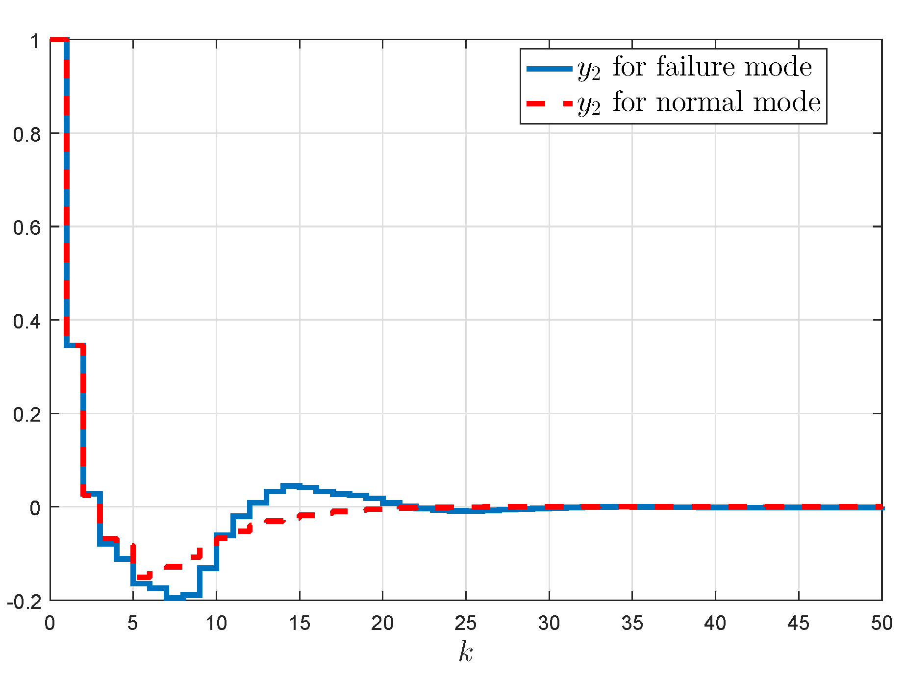
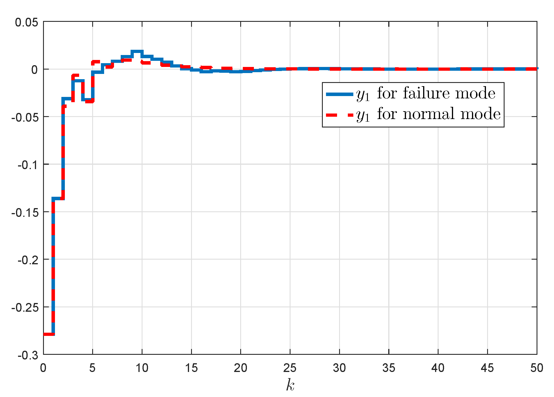
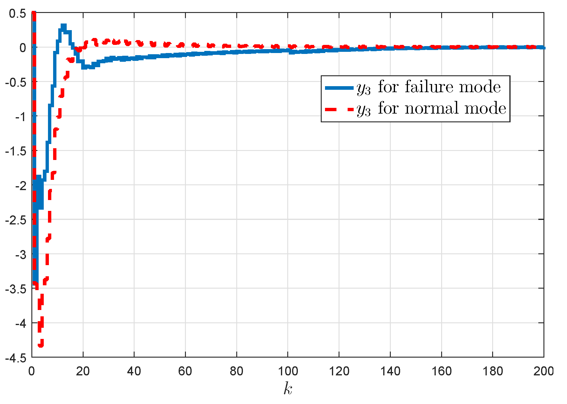
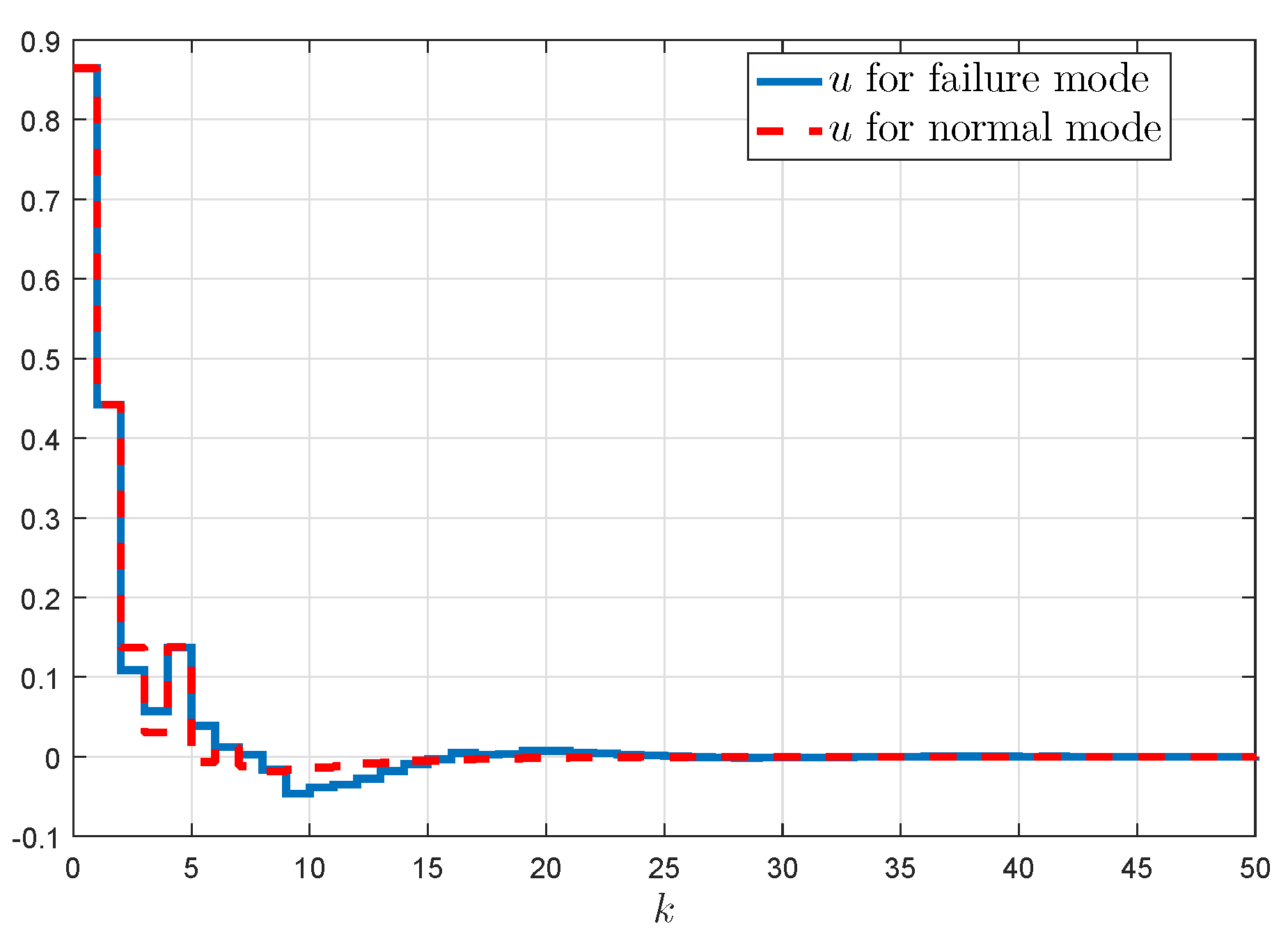
  • Normal mode, where reliable controller (91) is applied for a normal case without any failure;
  • Failure mode, where the proposed reliable controller (91) is implemented when the previous scenario affects the systems.
For both cases, the output and input responses of the closed-loop system are depicted in Figure 2, Figure 3, Figure 4 and Figure 5. As expected, the truck–trailer system is stabilized, despite the sensor failures and the stochastic external disturbances. Additionally, the simulation result provides potent verification for the effectiveness of the proposed control scheme in accommodating the effect of sensor faults on the system, and shows its robustness in spite of the external disturbances and uncertainties.
Example 3.
As it is mentioned that the proposed control design is also suitable for standard systems. Based on the ball and beam system, we make a comparison with the design method suggested in [42]. The ball and beam system is described by the following dynamic equations:
x ˙ 1 ( t ) = x 2 ( t ) x ˙ 2 ( t ) = b x 1 ( t ) x 4 2 ( t ) g sin ( x 3 ( t ) ) x ˙ 3 ( t ) = x 4 ( t ) x ˙ 1 ( t ) = u ( t ) + w ( t )
Set b = 0.7413 , g = 9.81 and h = 0.1 s as the sampling time. According to Euler’s discretization method, we can obtain the following discrete-time dynamic system:
x 1 ( k + 1 ) = x 1 ( k ) + h x 2 ( k ) x 2 ( k + 1 ) = x 2 ( k ) + h b x 1 ( k ) x 4 2 ( k ) g sin ( x 3 ( k ) ) x 3 ( k + 1 ) = x 3 ( k ) + h x 4 ( k ) x 4 ( k + 1 ) = x 2 ( k ) + h u ( k ) + h w ( k )
Assume that x 3 ( k ) π 2 π 2 and η ( k ) = x 1 ( k ) x 4 ( k ) 5 5 . Using the sector non-linearity approach, the TS fuzzy system can be established as follows:
x ( k + 1 ) = i = 1 2 h i ( η ( k ) ) A i x ( k ) + A d i x ( k d k ) + B 2 i u ( k ) + B 1 i w ( k ) + H f ( x ( k ) )
where A i = c A ¯ i , A d i = ( 1 c ) A ¯ i ,
A ¯ 1 = 1 h 0 0 0 1 2 π h b g h b d 0 0 1 h 0 0 0 1 , A ¯ 2 = 1 h 0 0 0 1 2 π h b g h b d 0 0 1 h 0 0 0 1 , B 2 i = B 1 i = 0 0 0 h , H = 0 h b g 0 0
The corresponding fuzzy membership functions are given as the following: h 1 ( η ( k ) ) = η ( k ) + 5 10 and h 2 ( η ( k ) ) = 5 η ( k ) 10 , while the non-linear function, f ( x ( k ) ) = sin ( x 3 ( k ) ) 2 π x 3 ( k ) , is bounded by the following:
Φ 1 = 0 0 0 0 , Ψ 1 = 0 0 1 2 π 0
Sensor faults are presented in Figure 6, and the uncertain parameters are assumed to be the following:
M = 0 0 h b g 0 T , N i = 0 0 1 2 π 0 , i = 1 , 2
Set c = 0.9 , d m = 1 , d M = 5 , γ = 0.8 , ϕ = 0 , K 1 0 = 1 2 10 4 , and K 2 0 = 1 1 4 4 . Assume that the sensor fault matrix R ( k ) satisfies diag { 0.7 , 0.6 , 0.5 , 0.4 } R ( k ) diag { 1 , 1.2 , 1.1 , 0.8 } . Using the CCL algorithm, the controller gains can be computed as the following:
K 1 = 0.69932 1.2392 16.079 8.0539
K 2 = 0.67935 1.7565 18.647 12.525
At this point, simulation studies are implemented with the initial condition x ( 0 ) = 1 0.2 0.9 0.1 T , and external disturbance selected as follows:
w ( k ) = 2 1 k 3 0 e l s e .
The results of the simulation are depicted in Figure 7. It is clear from this figure that the suggested control law in (48) keeps the dynamic stability of the closed-loop system, even in the presence of the sensor faults, model uncertainties and external disturbances.
To further demonstrate the merit of the proposed control strategy, we perform, under the same conditions, a comparison with the method proposed in [42]. Figure 8 shows the state trajectories of the system, using the following control law
u ( k ) = i = 1 r h i R ( k ) K a i x ( k d k ) + K b i f ( x ( k ) )
with the following gains
K a 1 = 0.0167 0.0005 0.0350 0.0152 , K b 1 = 0.7476 K a 2 = 0.0763 0.0335 0.0074 0.0298 , K b 2 = 0.2672
From this figure, it is clear that the control law developed in [42] may be incapable of dealing with a complex case, where the sensor faults and random non-linearity occur. Hence, the synthesized control law shows its superiority, compared to that proposed in [42].

6. Conclusions

In this paper, a new control scheme is developed for solving the main challenges faced while controlling discrete-time singular systems, such as the time-varying delay, randomly occurred non-linearities and sensor failures. Based on the TS fuzzy models and the Lyapunov–Krasovskii functional, the admissibility analysis is firstly studied by combining the delay decomposition and the reciprocally convex combination approaches. Then, a reliable static output feedback controller is designed such that the stability of the closed-loop system is ensured with accommodation of the negative effect caused by the sensors faults and noise. The feasibility of the addressed control problem is proved by establishing sufficient conditions such that the prescribed mixed H /passive performance level is achieved. The design of the controller gain is characterized by solving the CCL algorithm. Finally, the effectiveness of theoretical developments is verified by three examples. It should also be mentioned that many interesting types of research should be carried out in the future for Markovian jump singular systems described by interval type-2 fuzzy models with actuator/sensors faults, time-varying delay, and unknown transition probabilities.

Author Contributions

Conceptualization, M.K. and H.J.; methodology, M.K.; software, M.K. and H.J.; validation, M.K. and M.A.R.; formal analysis, M.K. and M.A.R.; investigation, A.B. and H.J.; resources, M.K. and A.L.K.; data curation, S.B.A. and H.J.; writing—original draft preparation, M.K. and M.A.R.; writing—review and editing, M.K. and M.A.R.; visualization, M.K. and M.A.R.; supervision, M.K., A.B. and H.J.; project administration, A.B.; funding acquisition, A.B. All authors have read and agreed to the published version of the manuscript.

Funding

This research was funded by a Research Deanship at the University of Ha’il, Saudi Arabia through project number RG20097.

Institutional Review Board Statement

Not applicable.

Informed Consent Statement

Not applicable.

Data Availability Statement

Data are contained within the article.

Acknowledgments

This research was funded by Scientific Research Deanship at University of Ha’il-Saudi Arabia through project number RG20097.

Conflicts of Interest

The authors declare no conflict of interest.

References

  1. Dai, L. Singular Control Systems. In Lecture Notes in Control and Information Sciences; Springer: New York, NY, USA, 1989; Volume 118. [Google Scholar]
  2. Duan, G. Analysis and Design of Descriptor Linear Systems; Springer: New York, NY, USA, 2010. [Google Scholar]
  3. Liu, Y.; Ma, Y.; Wang, Y. Reliable sliding mode finite-time control for discrete-time singular Markovian jump systems with sensor fault and randomly occurring nonlinearities. Int. J. Robust Nonlinear Control 2018, 28, 381–402. [Google Scholar] [CrossRef]
  4. Long, S.; Zhong, S. H control for a class of discrete-time singular systems via dynamic feedback controller. Appl. Math. Lett. 2016, 58, 110–118. [Google Scholar] [CrossRef]
  5. Ma, S.; Cheng, Z.; Zhang, C. Delay-dependent robust stability and stabilisation for uncertain discrete singular systems with time-varying delays. IET Control Theory Appl. 2007, 1, 1086–1095. [Google Scholar] [CrossRef]
  6. Zeng, Y.; Han, C.; Na, Y.; Lu, Z. Fuzzy-model-based admissibility analysis for nonlinear discrete-time descriptor system with time-delay. Neurocomputing 2016, 189, 80–85. [Google Scholar] [CrossRef]
  7. Fang, M. Delay-dependent stability analysis for discrete singular systems with time-varying delays. Acta Autom. Sin. 2010, 36, 751–755. [Google Scholar] [CrossRef]
  8. Wu, Z.; Park, J.H.; Su, H.; Chu, J. Admissibility and dissipativity analysis for discrete-time singular systems with mixed time-varying delays. Appl. Math. Comput. 2012, 2018, 7128–7138. [Google Scholar] [CrossRef]
  9. Seuret, A.; Gouaisbaut, F. Wirtinger-based integral inequality: Application to time-delay systems. Automatica 2013, 49, 2860–2866. [Google Scholar] [CrossRef] [Green Version]
  10. Feng, Z.; Li, W.; Lam, J. New admissibility analysis for discrete singular systems with time-varying delay. Appl. Math. Comput. 2015, 265, 1058–1066. [Google Scholar] [CrossRef]
  11. Chen, J.; Lin, C.; Chen, B.; Wang, Q.G. Fuzzy-model-based admissibility analysis and output feedback control for nonlinear discrete-time systems with time-varying delay. Inf. Sci. 2017, 412–413, 116–131. [Google Scholar] [CrossRef]
  12. Kchaou, M. Robust H Observer-Based Control for a Class of (TS) Fuzzy Descriptor Systems with Time-Varying Delay. Int. J. Fuzzy Syst. 2017, 19, 909–924. [Google Scholar] [CrossRef]
  13. Regaieg, M.A.; Kchaou, M.; El Hajjaji, A.; Chaabane, M. Robust H guaranteed cost control for discrete-time switched singular systems with time-varying delay. Optim. Control Appl. Methods 2019, 40, 119–140. [Google Scholar] [CrossRef]
  14. Samorn, N.; Yotha, N.; Srisilp, P.; Mukdasai, K. LMI-Based Results on Robust Exponential Passivity of Uncertain Neutral-Type Neural Networks with Mixed Interval Time-Varying Delays via the Reciprocally Convex Combination Technique. Computation 2021, 9, 70. [Google Scholar] [CrossRef]
  15. Takagi, T.; Sugeno, M. Fuzzy identification of systems an its application to modelling and control. Trans Syst. Man Cybern. 1985, 15, 116–132. [Google Scholar] [CrossRef]
  16. Latrach, C.; Kchaou, M.; Rabhi, A.; El Hajjaji, A. Decentralized networked control system design using Takagi-Sugeno (TS) fuzzy approach. Int. J. Autom. Comput. 2015, 12, 125–133. [Google Scholar] [CrossRef] [Green Version]
  17. Tanaka, K.; Wang, H. Fuzzy Control Systems Design and Analysis. A Linear Matrix Inequality Approach; Wiley: New York, NY, USA, 2001; p. 320. [Google Scholar]
  18. Li, W.; Feng, Z.; Sun, W.; Zhang, J. Admissibility analysis for Takagi–Sugeno fuzzy singular systems with time delay. Neurocomputing 2016, 205, 336–340. [Google Scholar] [CrossRef]
  19. Yang, P.; Ma, Y.; Yang, F.; Wang, D.K.L. Passivity control for uncertain singular discrete T-S fuzzy time-delay systems subject to actuator saturation. Int. J. Syst. Sci. 2018, 49, 1627–1640. [Google Scholar] [CrossRef]
  20. Ma, Y.; Yang, P.; Zhang, Q. Robust H control for uncertain singular discrete TS fuzzy time-delay systems with actuator saturation. J. Frankl. Inst. 2016, 353, 3290–3311. [Google Scholar] [CrossRef]
  21. Balasubramaniam, P.; Nagamani, G.; Rakkiyappan, R. Passivity analysis for neural networks of neutral type with Markovian jumping parameters and time delay in the leakage term. Commun. Nonlinear Sci. Numer. Simul. 2011, 16, 4422–4437. [Google Scholar] [CrossRef]
  22. Liang, J.; Wang, Z.; Liu, X. On Passivity and Passification of Stochastic Fuzzy Systems With Delays:The Discrete-Time Case. IEEE Trans. Syst. Man Cybern. Part B 2010, 40, 964–969. [Google Scholar] [CrossRef] [PubMed] [Green Version]
  23. Wu, Z.; Park, J.; Su, H.; Song, B.; Chu, J. Mixed H and passive filtering for singular systems with time delays. Signal Process. 2013, 93, 1705–1711. [Google Scholar] [CrossRef]
  24. Liu, Z.; Karimi, H.R.; Yu, J. Passivity-based robust sliding mode synthesis for uncertain delayed stochastic systems via state observer. Automatica 2020, 111, 108596. [Google Scholar] [CrossRef]
  25. Zheng, Q.; Ling, Y.; Wei, L.; Zhang, H. Mixed H and passive control for linear switched systems via hybrid control approach. Int. J. Syst. Sci. 2018, 49, 818–832. [Google Scholar] [CrossRef]
  26. Chen, J.; Lin, C.; Chen, B.; Wang, Q. Mixed H and passive control for singular systems with time delay via static output feedback. Appl. Math. Comput. 2017, 293, 244–253. [Google Scholar] [CrossRef]
  27. Zhu, M.; Chen, Y.; Kong, Y.; Chen, C.; Bai, J. Distributed filtering for Markov jump systems with randomly occurring one-sided Lipschitz nonlinearities under Round-Robin scheduling. Neurocomputing 2020, 417, 396–405. [Google Scholar] [CrossRef]
  28. Ji, H.; Zhang, H.; Li, C.; Senping, T.; Lu, J.; Wei, Y. H control for time-delay systems with randomly occurring nonlinearities subject to sensor saturations, missing measurements and channel fadings. ISA Trans. 2018, 75, 38–51. [Google Scholar] [CrossRef]
  29. Zhang, Y.; Jiang, J. Bibliographical review on reconfigurable fault-tolerant control systems. Annu. Rev. Control 2008, 32, 229–252. [Google Scholar] [CrossRef]
  30. Sakthivel, R.; Selvi, S.; Mathiyalagan, K.; Shi, P. Reliable Mixed H and Passivity-Based Control for Fuzzy Markovian Switching Systems with Probabilistic Time Delays and Actuator Failures. IEEE Trans. Cybern. 2015, 45, 2720–2731. [Google Scholar] [CrossRef]
  31. Chang, X.; Zhang, L.; Park, J. Robust static output feedback H control for uncertain fuzzy system. Fuzzy Sets Syst. 2015, 87–104, 273. [Google Scholar]
  32. Zhang, D.; Zhou, Z.; Jia, X. Networked fuzzy output feedback control for discrete-time Takagi-Sugeno fuzzy systems with sensor saturation and measurement noise. Inf. Sci. 2018, 457–458, 182–194. [Google Scholar] [CrossRef]
  33. Wang, L.; Du, H.; Wu, C.; Li, H. New Compensation for Fuzzy Static Output-Feedback Control of Nonlinear Networked Discrete-Time Systems. Signal Process. 2016, 120, 255–265. [Google Scholar] [CrossRef]
  34. Khalil, H. Nonlinear Systems; Prentice-Hall: Hoboken, NJ, USA, 1996. [Google Scholar]
  35. Xu, S.; Lam, J. Robust Control and Filtering of Singular Systems; Springer: Berlin/Heidelberg, Germany, 2006. [Google Scholar]
  36. Petersen, I. A stabilization algorithm for a class of uncertain linear systems. Syst. Control Lett. 1987, 8, 35–357. [Google Scholar] [CrossRef]
  37. Park, P.; Ko, J.; Jeong, C. Reciprocally convex approach to stability of systems with time-varying delays. Automatica 2011, 47, 235–238. [Google Scholar] [CrossRef]
  38. Wu, Z.; Shi, P.; Su, H.; Chu, J. Delay-dependent stability analysis for discrete-time singular Markovian jump systems with time-varying delay. Int. J. Syst. Sci. 2012, 43, 2095–2106. [Google Scholar] [CrossRef]
  39. Tuan, H.; Apkarian, P.; Narikiyo, T.; Yamamoto, Y. Parameterized linear matrix inequality techniques in fuzzy control system design. IEEE Trans. Fuzzy Syst. 2001, 9, 324–332. [Google Scholar] [CrossRef] [Green Version]
  40. Ghaoui, L.E.; Oustry, F.; Ait-Rami, R. A cone complementarity linearization algorithm for static output-feedback and related problems. IEEE Trans. Autom. Control 1997, 42, 1171–1176. [Google Scholar] [CrossRef] [Green Version]
  41. Chang, J.L.; Lin, M.L. Observer-Based robust H control for fuzzy systems using two-step procedure. IEEE Trans. Fuzzy Syst. 2004, 12, 350–359. [Google Scholar]
  42. Sakthivel, R.; Sundareswari, K.; Mathiyalagan, K.; Santra, S. Reliable H Stabilization of Fuzzy Systems with Random Delay Via Nonlinear Retarded Control. Circuits Syst. Signal Process. 2016, 35, 1123–1145. [Google Scholar] [CrossRef]
Figure 1. Flowchart of the control procedure.
Mathematics 09 02203 g001
Figure 2. The response of system output variable y 1 .
Mathematics 09 02203 g002
Figure 3. The response of system output variable y 2 .
Mathematics 09 02203 g003
Figure 4. The response of system output variable y 3 .
Mathematics 09 02203 g004
Figure 5. The response of system control input u.
Mathematics 09 02203 g005
Figure 6. Sensor faults model.
Mathematics 09 02203 g006
Figure 7. State trajectories in case 1.
Mathematics 09 02203 g007
Figure 8. State trajectories in case 2.
Mathematics 09 02203 g008
Table 1. Calculated maximum d M for various d m .
Methods d m = 3 d m = 6 d m = 9 d m = 12
[5]8101315
[6]15161719
[7]16192225
[8]19212427
[9]28303336
[10]37394244
[11]45454851
Theorem 152495053
Publisher’s Note: MDPI stays neutral with regard to jurisdictional claims in published maps and institutional affiliations.

