Stability Analysis of Systems with Fuzzy PI Controllers Applied to Electric Drives

Abstract

This paper analyzes the stability of fuzzy control systems with applications for electric drives. Ensuring the stability of these systems is a necessity in practice. The purpose of the study is the analysis of the dynamic characteristics of the speed control systems of electric drives based on fuzzy PI controllers in the context of performing stability analyses, both internal and input–output, finding solutions to stabilize these systems and provide guidance on fuzzy regulator design. The main methods of treatment applied are as follows: framing the control system in the theory of stability of multivariable non-linear systems, application of Lyapunov’s theory, performing an input–output stability analysis, and verification of the stability domain. The article presents the conditions for correcting the fuzzy controller to ensure internal and external stability, determines the limits of the stability sector, and gives indications for choosing the parameters of the controller. The considerations presented can be applied to various structures for regulating the speed of electric drives which use various PI fuzzy controllers.

1. Introduction

The study presented in this paper fits into the broader context of the mathematics of fuzzy controllers, Mamdani structures, and the control of electric drives, as well as the industrial application of fuzzy control systems. Various scientific papers have appeared in the literature for many years, presenting examples of the use of fuzzy logic in regulating the speed of electric drives [1,2]. The paper [3] addresses a variety of issues related to advances in control techniques for electric drives in emerging fields such as electric vehicles, UAVs, trains, and motion control. Fuzzy logic is an instrument of artificial intelligence which translates human reasoning into numerical calculations [4,5]. In these studies, there are particular cases of the use of fuzzy PI regulators. In practice, however, their widespread application in commercial equipment to control electric drives is hampered by a number of impediments, such as the lack of precise methods for designing control systems based on fuzzy logic, the lack of precise methods of stability analysis, based on which one can be confident that they can undoubtedly ensure a certain quality of stability of the control systems of electric drives, and, finally, the increased complexity of the development systems of driving equipment based on fuzzy logic.

The analysis of the stability of fuzzy control systems is approached in the literature by using various methods of analysis: utilization of a small-signal state-space linearized model [6] based on Lyapunov’s direct method [7,8], using the Toeplitz matrices and their singular values [9], analyzing input-to-state stability and imposing some conditions [10], and applying Lyapunov’s functions and theorem [11,12].

This paper provides solutions to eliminate the disadvantages in the implementation of speed regulators based on fuzzy blocks. The analysis performed in the paper is intended for various types of fuzzy block, made with various membership functions, fuzzyfication methods, rule bases, inferences, or defuzzification methods. In practice, many fuzzy blocks, which have a general Mamdani structure, meet the sector conditions necessary to ensure stability in accordance with the method of this paper. Several structures of fuzzy blocks that have three, five, and seven membership functions, rule bases with 3 × 3, 3 × 5, 5 × 5, and 5 × 7 fuzzy values, inferences with min–max and prod–sum methods, and defuzzification with the center of gravity meeting the sector conditions are necessary to ensure stability in accordance with the methods of this paper. The stability analysis performed will show which sector conditions the fuzzy blocks must meet to ensure the global asymptotic internal stability of speed control systems. Answering these questions, it will be possible to eliminate, at a later design stage, the empirical and unsystematic character of implementing the knowledge of the operator and of the synthesis of the speed regulator based on fuzzy logic. Another major disadvantage to which a solution is given is the impossibility of demonstrating the stability of fuzzy control systems in general in the absence of valid models for control systems based on fuzzy logic. Hence, it is impossible to determine the quality of the stability of the control system. In the design of control structures with regulators based on fuzzy logic, knowledge of automatic control engineering was applied, despite the opinion of some that the use of fuzzy logic is possible without any knowledge of the theory of control systems. No matter how much fuzzy logic-based control structures have been developed, as will be seen in the paper, one cannot advance without using knowledge from the theory of invariant linear and non-linear control systems, a theory that is strong and well-structured and that meets practical requirements. Due to the fact that control structures based on fuzzy logic can only be implemented by using digital equipment, such as fast digital signal processors, it is necessary to use the theory of digital control systems and apply theories for quasi-continuous systems.

The paper is further structured into four sections: preliminaries, stability analysis, discussions, and conclusions. The steps followed in the stability analysis procedure are presented below, in a step-by-step flowchart.

Steps	Results
Determination of the mathematical model of the regulation system	Block diagram of the control system, mathematical models of the components (motor, converter, sensors), parameter values
Determination of the fuzzy PI controller model	Block diagram of the fuzzy controller Calculation of the transfer characteristics of the fuzzy non-linear block Equivalence of the mathematical model of the fuzzy regulator Designing the coefficients of the fuzzy regulator
Construction of the block scheme for stability analysis	Calculation of the mathematical model for stability analysis Calculation of the transfer characteristics of the non-linear part
Analysis of the steady-state regime	Calculation of the steady-state regime values for the system variables
Analysis of the state portrait of the rule base	Demonstration of the existence of stable state trajectories
Calculation of the root locus of the linear part	Calculation of the poles and zeros of the linear part Determination of the shape of the root locus
Correction of the non-linear part	Calculation of the transfer characteristics of the corrected non-linear part
Calculation of the range of variation of the limits of the stability sector in which the non-linearity falls	Calculation of the minimum and maximum values of the sector domain
Construction of the block diagram for the analysis of internal stability	Calculation of its mathematical model
Application of the Kalman–Yakubovich–Popov lemma	Determination of the positively defined function
Demonstration of internal stability applying Lyapunov’s method	Choosing the Lyapunov function Demonstration of absolute global internal stability
Application of the circle criterion	Construction of the linear part hodograph. Location of the circle
The procedure for correcting the characteristics of non-linearity and determining the stability sector	Indication for correcting the sector limits
Simulation testing of the limits of the stability sector	Determining the transient regime characteristics for various values of the scaling coefficient
Demonstration of the external bounded-input bounded-output (BIBO) stability	Determining the equations of the regulation system for the analysis of the input–output stability Demonstration of the fulfillment of the conditions for BIBO external stability Verification by simulation of the BIBO external stability of the control system

2. Preliminaries

2.1. Control Structure

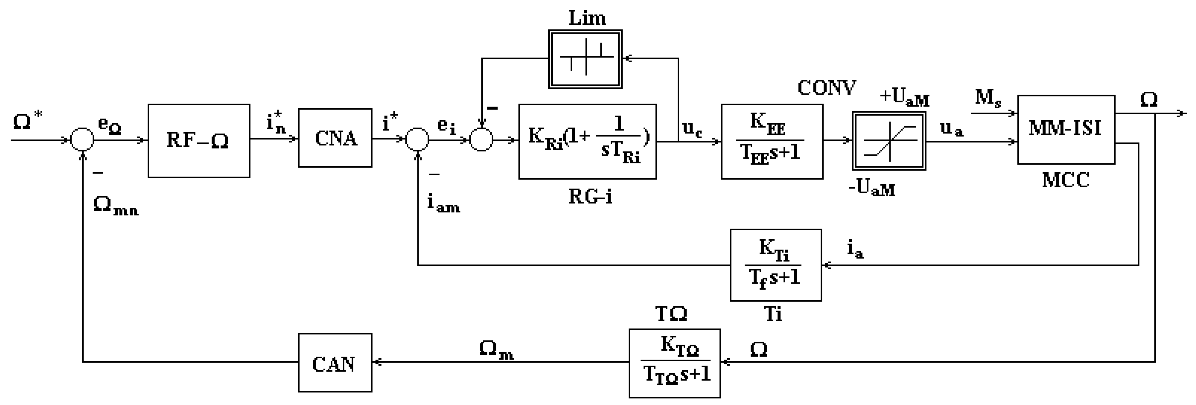
Figure 1 shows the speed control structure of the electric drive, with a speed regulator based on fuzzy logic [13,14].

The meaning of the notations in the figure is as follows: MCC—DC motor, MM-ISI—motor state-space equations, M_s—load torque, Ω—rotational speed, u_a—armature voltage, +/−U_aM—armature voltage limitations, CONV—electronic power convertor, K_EE—convertor gain, T_EE—convertor time constant, s—Laplace transformation complex variable, u_c—control variable from the current controller, RG-i—current controller, K_RGi—current controller gain, T_Ri—integrating time constant of the current regulator, Lim—non-linear limiting block with anti-wind-up effect, e_i—current error, CNA—digital to analog convertor, i*—analog current reference, i_a*—digital current reference, RF-Ω—fuzzy speed controller, e_Ω—speed error, Ω*—speed reference, Ω_mn—digital measured speed, CAN—analog to digital converter, TΩ—speed sensor, K_TΩ—speed sensor gain, T_TΩ—speed sensor time constant. The speed control structure was classic [15], and it replaced the linear PI speed controller with a fuzzy PI controller. The current control loop was dimensioned based on the modulus optimum criterion, in the Kessler version [16].

The DC motor has the equations:

$$\begin{array}{c}{u}_a=R_a{i}_a+L_a\frac{d{i}_a}{dt}+e\\ J\frac{d\mathsf{\Omega }}{dt}=M-k_f\mathsf{\Omega }-M_s\end{array}$$

(1)

where

$$\begin{array}{c}e=k_e\mathsf{\Omega }\\ M=k_m{i}_a\end{array}$$

(2)

The motor parameters are as follows: P_n = 1 kW, U_n = 220 V, n_n = 3000 rot./min, η = 0.75, p = 2, J = 0.006 kgm², M_n = P_n/Ω_n = 3.2 Nm, Ω_n = 2 πn_n/60 = 314 rad/s, I_n = P_n/η/U_n = 6 A, I_M = I_lim = 1.8 I_n = 10.8 A, R_a = 0.055 U_n/I_n = 2.01 Ω, L_a = 5.6 U_n/n_n/p/I_n = 0.034 H, T_a = L_a/R_a = 0.017 ms, k_e = (U_n − I_nR_a)/Ω_n = 0.664 Vs, k_m = M_n/I_n = 0.533 Nm/A, k_f = 0.08 M_n/Ω_n = 8.10⁻⁴ Nms. The parameters of the current regulator, those of the power converter and of the current and speed sensors are: K_RGi = 0.2, T_RGi = T_a = 0.017 ms, K_EE = 22, T_EE = 0.8 ms, K_Ti = 1 A⁻¹, T_Ti = 4 ms, K_TΩ = 0.1 π/Vs, T_TΩ = 10 ms. The analog-to-digital and digital-to-analog converters used in the control structure were considered to be 12 bits and have a maximum analog voltage of 10 V. In this case, for the values of the amplifications introduced by these converters, the following values resulted as: K_CAN = 211/10 = 204.8 bit/Volt and K_CNA = 1/KCAN = 0.0049 Volt/bit.

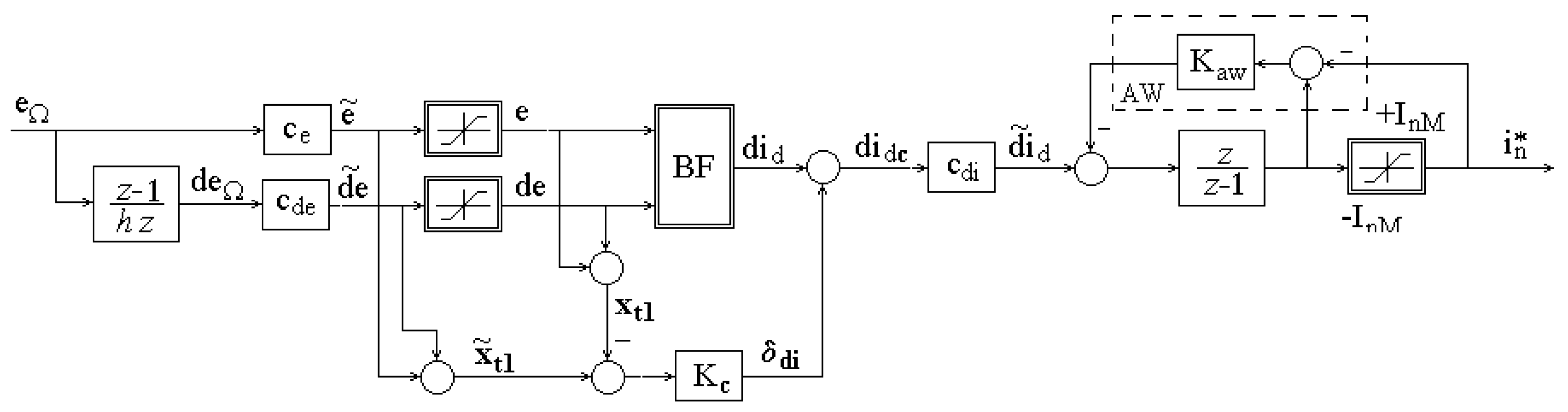
2.2. Speed Fuzzy PI Controller

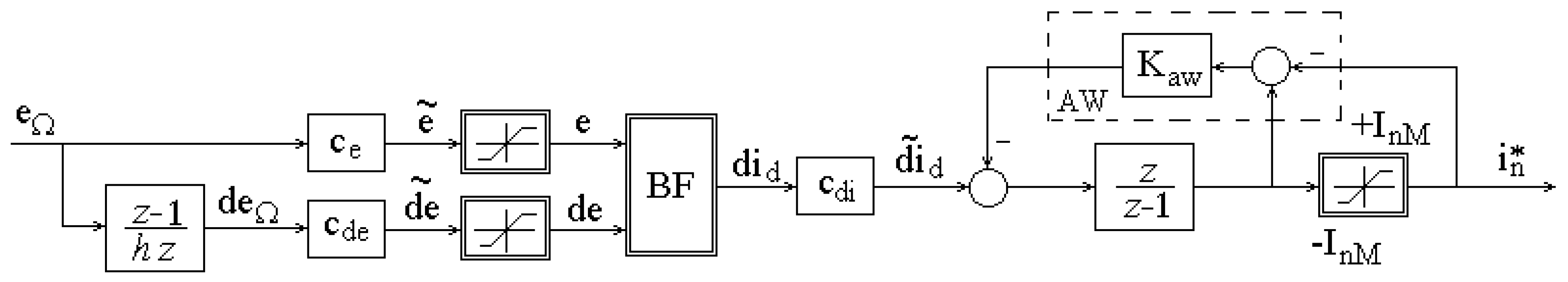
The block diagram of the speed controller based on fuzzy logic had a structure as shown in Figure 2 [17,18,19].

The speed controller is a PI fuzzy controller with integration (summation) at the output. A circuit with a negative reaction anti-wind-up, denoted AW, was introduced in this scheme. The meanings of the notations in the figure are as follows: e_Ω—speed error, de_Ω—error derivative, c_e and c_de—scaling coefficients, BF—fuzzy block, di_d—defuzzified value, current increment, c_di—control output gain, K_AW—gain coefficient, +/−I_nM—the maximum limit current prescribed in transient regime, i_n*—digital current reference, e, de—fuzzy block inputs. The values at the fuzzy bloc inputs are scaled in the universes of discourse.

For the amplification coefficients c_e and c_de, from the two inputs of the fuzzy block, values obtained by a pseudo-equivalence of the fuzzy PI regulator with a linear PI regulator dimensioned with the symmetrical optimal criterion in Kessler’s variant were adopted, after iterative tests.

2.3. Transfer Characteristics of the Fuzzy Block

The fuzzy block BF from Figure 2 may be developed using Mamdani’s structure, with different membership functions, fuzzyfication methods, rule bases, inference methods and defuzzification methods [17,18,19]. In this paper, an example of fuzzy block with membership functions from Figure 3a, a rule base with nine rules, min–max inference and defuzzification with center of gravity is taken in consideration. It has the highest non-linear character. Its transfer characteristics are presented in Figure 3b–d, where x_t1 = e + de [17,18,19].

2.4. Pseudo-Equivalence of the Fuzzy PI Controller

A pseudo-equivalence with a linear PI controller is used to design the fuzzy PI controller, in accordance with [20,21,22,23]. The fuzzy block BF is linearized around the steady state operating point: (e = 0, de = 0, di_d = 0). Its output is given by Equation (3):

$$d{i}_d=K_0(e+de)$$

(3)

K₀ is calculated from the characteristic families K_BF = (x_t1; de) with Equation (4):

$$K_0=\underset{x_{t1}\to 0}{\lim }{K}_{BF}(x_{t1}; 0)$$

(4)

The characteristic of the fuzzy block linearized around the origin is:

$$\widetilde{d{i}_d}=c_{di}{K}_0(e+de), {\tilde{c}}_{di}=c_{di}{K}_0$$

(5)

The transfer function of the fuzzy speed controller RF-Ω in the z domain is:

$$i_n^{*}(z)=\frac{z}{z-1}{\tilde{c}}_{di}[e(z)+de(z)]=\frac{z}{z-1}{\tilde{c}}_{di}\left[c_e+c_{de}\frac{z-1}{hz}\right]e_{\Omega }(z)$$

(6)

The transfer function of the fuzzy speed controller RF-Ω is:

$$H_{RF}(z)=\frac{i_n^{*}(z)}{e_{\Omega }(z)}=\frac{z}{z-1}{\tilde{c}}_{di}\left(c_e+c_{de}\frac{z-1}{hz}\right)$$

(7)

The linear PI controller has the transfer function:

$$H_{R\mathsf{\Omega }}\left(s\right)=K_{R\mathsf{\Omega }}\left(1+\frac{1}{s{T}_{R\mathsf{\Omega }}}\right)$$

(8)

With a quasi-continuous form:

$$H_{RF}(s)=\frac{i_n^{*}(s)}{e_{\Omega }(s)}={H_{RF}(z)|}_{z=\frac{1+sh/2}{1-sh/2}}=\frac{{\tilde{c}}_{di}}{h}\left(c_{de}+\frac{h}{2}{c}_e\right)\left[1+\frac{c_e}{(c_{de}+c_{e}h/2)s}\right]$$

(9)

In accordance with [20,21,22], the relationships for controller coefficients are:

$$c_e=\frac{h{K}_{R\Omega }}{c_{dM}{K}_0{T}_{R\Omega }}, c_{de}=c_e(T_{R\Omega }-h/2)$$

(10)

were h is the sampling period.

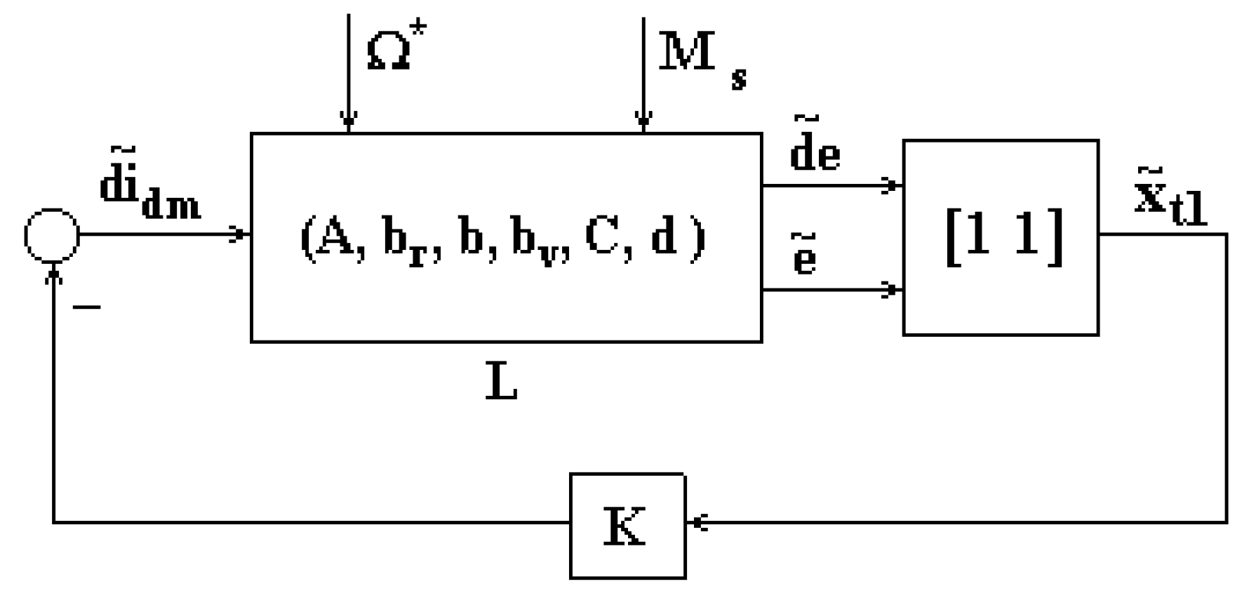
2.5. Model of the Control System Used in Stability Analysis

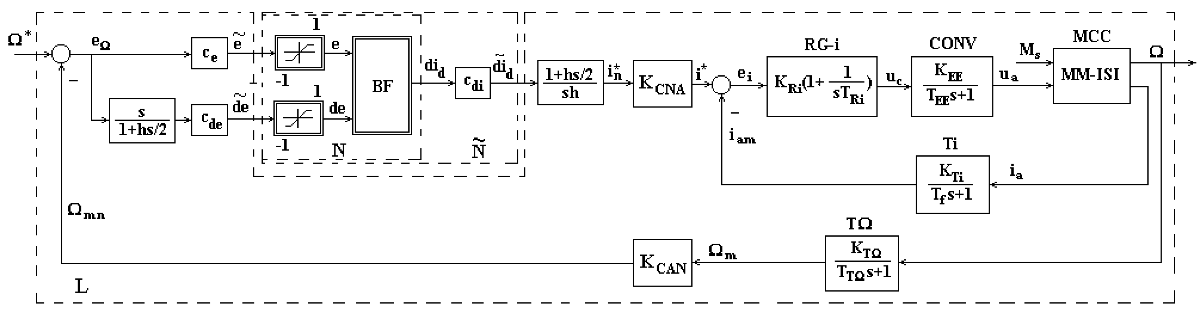
For the analysis of the stability of the speed control system of electric drives based on fuzzy speed controller, we worked with a quasi-continuous model of the control system, as shown in Figure 4.

The elements of derivation and numerical integration have been replaced by continuous transfer functions [20,21,22,23]. The sampling step was denoted by h.

The system from Figure 4 has the equations:

$$\begin{array}{c}{\dot{\Omega }}_{mn}=-\frac{1}{T_{T\Omega }}{\Omega }_{mn}+\frac{K_{CAN}{K}_{T\Omega }}{T_{T\Omega }}\Omega \\ {\dot{x}}_{a1}=-\frac{2c_{de}}{h}{\Omega }_{mn}-\frac{2}{h}{x}_{a1}+\frac{2c_{de}}{h}{\Omega }^{*}\\ \dot{\Omega }=-\frac{k_f}{J}\Omega +\frac{k_m}{J}{i}_a-\frac{1}{J}{M}_s\\ {\dot{i}}_a=-\frac{k_e}{L_a}\Omega -\frac{R_a}{L_a}{i}_a+\frac{1}{L_a}{u}_a\\ {\dot{u}}_a=-\frac{1}{T_{EE}}{u}_a+\frac{K_{EE}}{T_{EE}}{x}_{a2}-\frac{K_{EE}{K}_{Ri}}{T_{EE}}{i}_{am}+\frac{K_{EE}{K}_{Ri}}{T_{EE}}{x}_{a3}+\frac{K_{EE}{K}_{Ri}{K}_{CNA}}{2T_{EE}}{\widetilde{di}}_d\\ {\dot{x}}_{a2}=-\frac{K_{Ri}}{T_{Ri}}{i}_{am}+\frac{K_{Ri}}{T_{Ri}}{x}_{a3}+\frac{K_{Ri}{K}_{CNA}}{2T_{Ri}}{\widetilde{di}}_d\\ {\dot{i}}_{am}=-\frac{1}{T_f}{i}_{am}+\frac{K_{Ti}}{T_f}{i}_a\\ {\dot{x}}_{a3}=\frac{K_{CAN}}{h}{\widetilde{di}}_d\\ {\tilde{y}}_1=\tilde{e}=-c_e{\Omega }_{mn}+c_e{\Omega }^{*}\\ {\tilde{y}}_2=\widetilde{de}=-\frac{2c_{de}}{h}{\Omega }_{mn}-\frac{2}{h}{x}_{a1}+\frac{2c_{de}}{h}{\Omega }^{*}\\ {\widetilde{di}}_d=c_{di}d{i}_d=c_{di}{f}_{BF}(e,de)={\tilde{f}}_{\tilde{N}}(\tilde{e},\widetilde{de})\end{array}$$

(11)

where

$$\begin{array}{c}{x}_{a1}=c_{de}{e}_{\Omega }-\frac{h}{2}\widetilde{de}\\ e_{\Omega }={\Omega }^{*}-{\Omega }_{mn}\\ x_{a2}=u_c-K_{Ri}{e}_i\\ e_i=i^{*}-i_{am}\\ x_{a3}=i^{*}-\frac{K_{CNA}}{2}{\widetilde{di}}_d\end{array}$$

(12)

In the block diagram in Figure 3, the fuzzy block, BF, together with the saturated elements at its inputs form a nonlinear part are symbolized with N. The non-linear part N, with the increment coefficient of the current c_di, forms the global non-linearity $\tilde{N}$. The linear L part is formed by the rest of the blocks. In the structure in Figure 3, the block AW was not taken into account. In the above equations the fuzzy bloc is described by the two variable non-linear functions $f_{BF}(e,de)$, and ${\tilde{f}}_{\tilde{N}}(\tilde{e},\widetilde{de})$. The function of two variables of N is ${\tilde{f}}_{\tilde{N}}(\tilde{y})$.

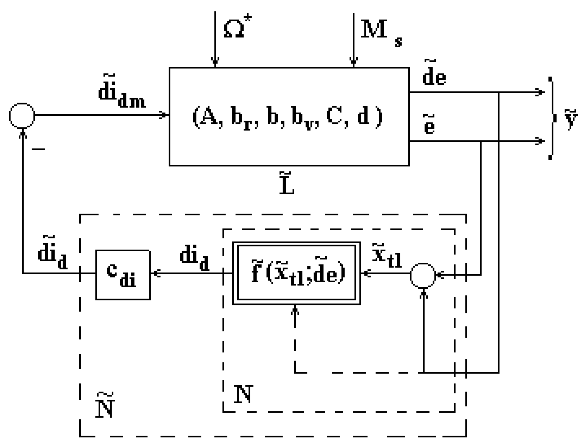
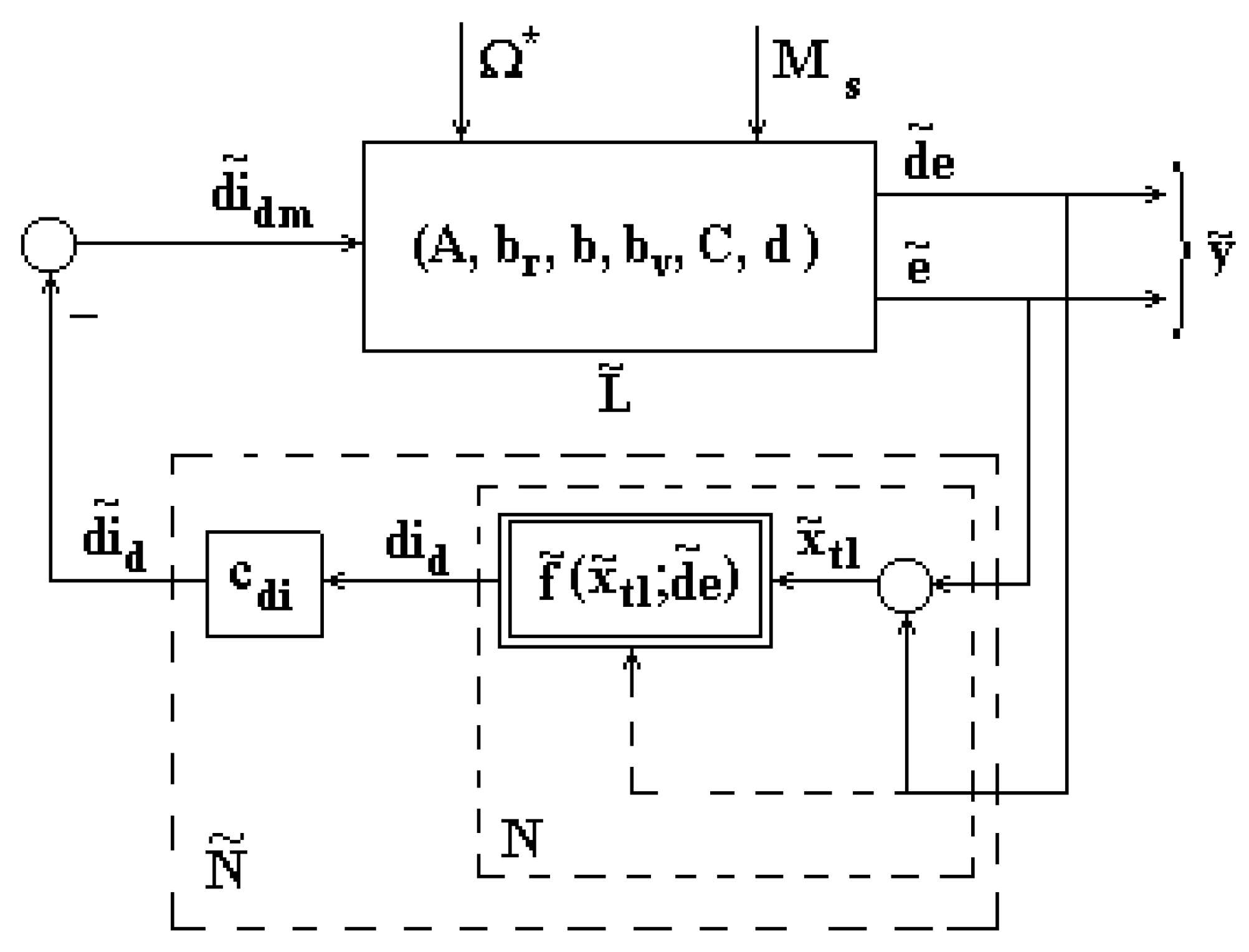
Figure 5 shows the structure of Figure 4, reconfigured into a structure specific to addressing the problem of absolute stability, recommended in [24,25,26,27], for systems with a non-linearity.

In Figure 5, the linear part $\tilde{L}$ has ${\widetilde{di}}_{dm}=-{\widetilde{di}}_d$ as an input variable. The block $\tilde{L}$ differs from the block L by the placement of an inverter block at the entrance. Its output is $\tilde{y}={[{\tilde{y}}_1 {\tilde{y}}_2]}^T={[\tilde{e} \widetilde{de}]}^T$. The non-linearity $\tilde{N}$ is placed in the negative feedback. The fuzzy block BF has the inputs $y={[y_1 y_2]}^T={[e de]}^T$. Equations (11) and (12) of the control system can be reproduced and concentrated, following the inserting of the input inverter block by the mathematical model:

$$\begin{array}{c}\dot{x}(t)=A·x(t)+b_r·{\widetilde{di}}_{dm}(t)+b·{\Omega }^{*}(t)+b_v·M_s(t)\\ \tilde{y}(t)=C·x(t)+d·{\Omega }^{*}(t)\\ {\widetilde{di}}_{dm}=-{\tilde{f}}_{\tilde{N}}(\tilde{e},\widetilde{de})=-c_{di}·d{i}_d\\ d{i}_d=f_N(\tilde{e},\widetilde{de})\end{array}$$

(13)

where

$$\begin{array}{c}x={\left[\begin{array}{cccccccc}{\Omega }_{mn}& x_{a1}& \Omega & i_a& u_a& x_{a2}& i_{am}& x_{a3}\end{array}\right]}^T\\ \tilde{y}={\left[\begin{array}{cc}\tilde{e}& \widetilde{de}\end{array}\right]}^T\\ A=\left[\begin{array}{cccccccc}-\frac{1}{T_{T\Omega }}& 0& \frac{K_{CAN}{K}_{T\Omega }}{T_{T\Omega }}& 0& 0& 0& 0& 0\\ -\frac{2c_{de}}{h}& -\frac{2}{h}& 0& 0& 0& 0& 0& 0\\ 0& 0& -\frac{k_f}{J}& \frac{k_m}{J}& 0& 0& 0& 0\\ 0& 0& -\frac{k_e}{L_a}& -\frac{R_a}{L_a}& \frac{1}{L_a}& 0& 0& 0\\ 0& 0& 0& 0& -\frac{1}{T_{EE}}& \frac{K_{EE}}{T_{EE}}& -\frac{K_{EE}{K}_{Ri}}{T_{EE}}& \frac{K_{EE}{K}_{Ri}}{T_{EE}}\\ 0& 0& 0& 0& 0& -\frac{K_{Ri}}{T_{Ri}}& 0& \frac{K_{Ri}}{T_{Ri}}\\ 0& 0& 0& 0& 0& 0& -\frac{1}{T_f}& \frac{K_{Ti}}{T_f}\\ 0& 0& 0& 0& 0& 0& 0& 0\end{array}\right]\\ b_r={\left[\begin{array}{cccccccc}0& 0& 0& 0& -\frac{K_{EE}{K}_{Ri}{K}_{CNA}}{2T_{EE}}& -\frac{K_{Ri}{K}_{CNA}}{2T_{Ri}}& 0& -\frac{K_{CNA}}{h}\end{array}\right]}^T\\ b={\left[\begin{array}{cccccccc}0& \frac{2c_{de}}{h}& 0& 0& 0& 0& 0& 0\end{array}\right]}^T\\ b_v={\left[\begin{array}{cccccccc}0& 0& -\frac{1}{J}& 0& 0& 0& 0& 0\end{array}\right]}^T\\ C=\left[\begin{array}{cccccccc}-c_e& 0& 0& 0& 0& 0& 0& 0\\ -\frac{2c_{de}}{h}& -\frac{2}{h}& 0& 0& 0& 0& 0& 0\end{array}\right]\\ d={\left[\begin{array}{cc}{c}_e& \frac{2c_{de}}{h}\end{array}\right]}^T\end{array}$$

(14)

The non-linear function of two variables was attached to the fuzzy block:

$$d{i}_d=f_{BF}(e,de)$$

(15)

with the universes of discourse U_e, U_de and U_di from Figure 3a.

With the compound variable x_t1:

$$x_{t1}=\left[\begin{array}{cc}1& 1\end{array}\right]y=e+de$$

(16)

and the function of variable x_t1 and parameter de:

$$K_{BF}(x_{t1};de)=\frac{f_{BF}(e,de)}{x_{t1}},\hspace{1em}{x}_{t1}\ne 0$$

(17)

the variable di_d is expressed under the form:

$$d{i}_d=\{\begin{array}{l}{K}_{BF}(x_{t1};de)x_{t1} ,\hspace{1em}pt.\hspace{1em}{x}_{t1}\ne 0\\ 0,\hspace{1em}pt.\hspace{1em}{x}_{t1}=0\end{array}$$

(18)

The families of characteristics d_id = f(x_t1; de), from Figure 3c, have the property that they are only in quadrants I and III [20,21,22].

The values of the function K_BF(x_t1; de) may be determined from the family of characteristics from Figure 3d [20,21,22]. This family of characteristics induces the need for the relationship:

$$0\le K_{BF}(x_{t1};de)\le K_M$$

(19)

The values of K_M may be determined from Figure 3d [17,18,19].

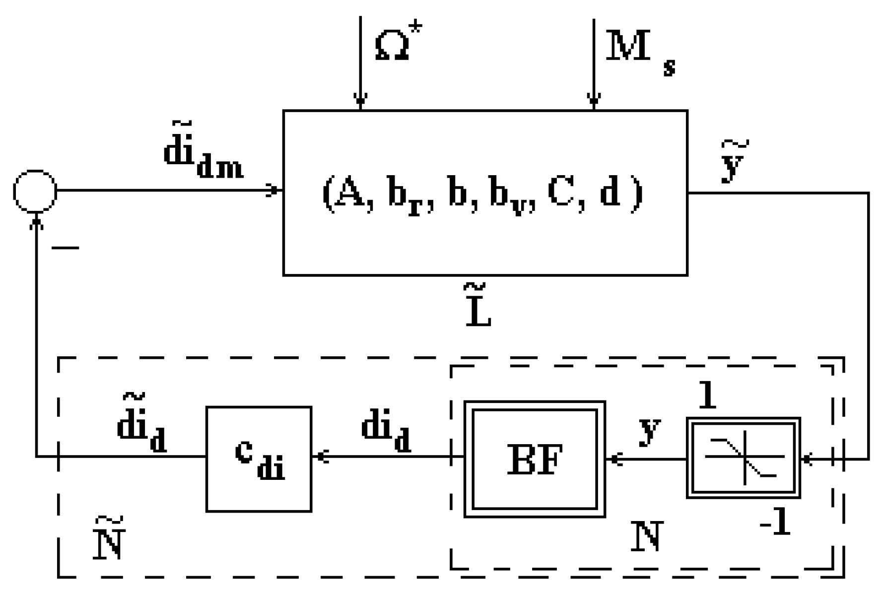
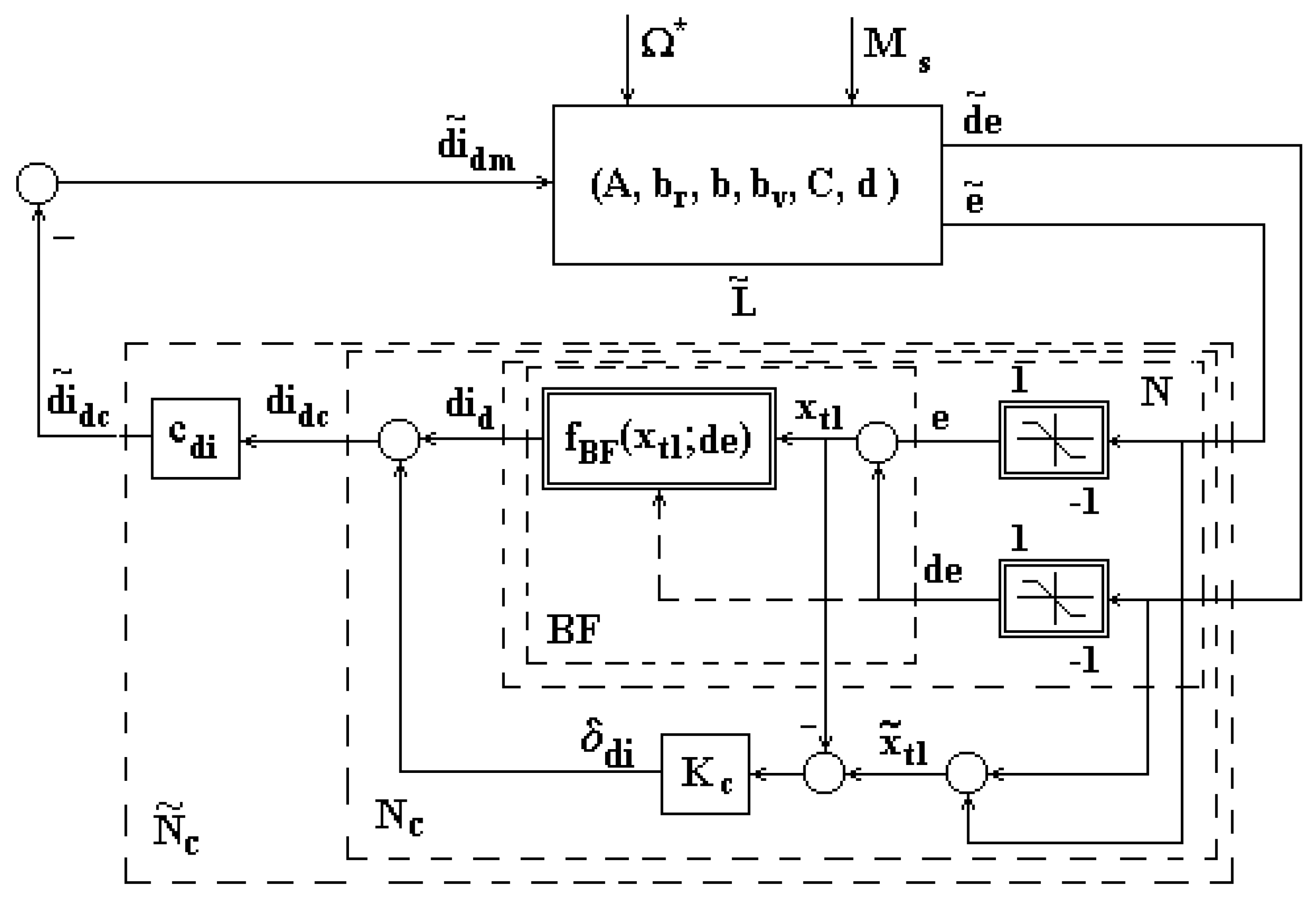
The new structure obtained from Figure 5 after the transformation with the Equations (16)–(18) is presented in Figure 6.

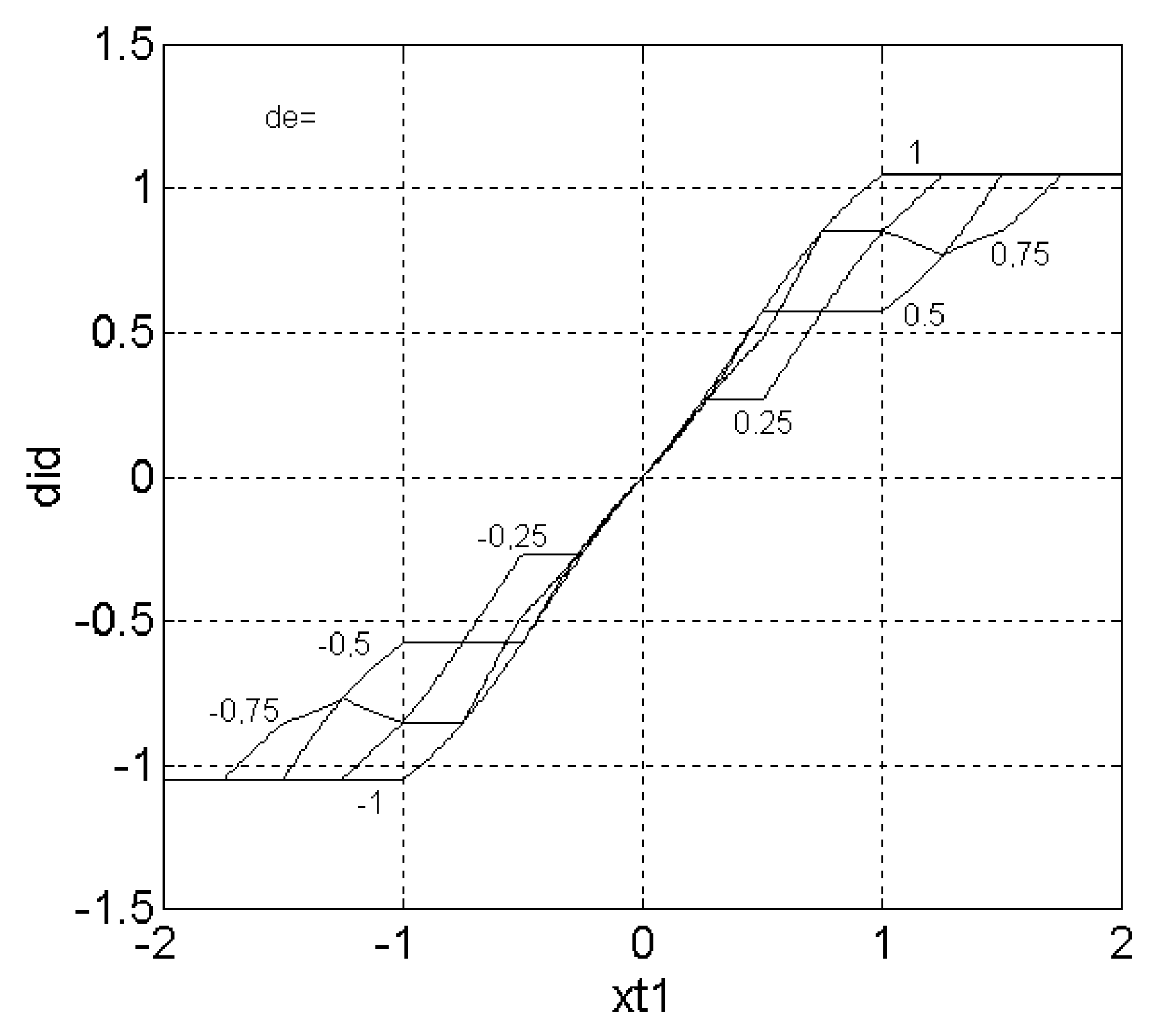
The fuzzy block works on the discourse universe [−1, 1], $x_{t1}\in \left[-2, 2\right]$. The family of characteristics di_d = f (x_t1; de) is shown in Figure 7.

If the fuzzy block is working on the extended universe of discourse, the “indeterminacy syndrome” appears. This is due to the saturations of the membership functions at the extremities of universes of discourse. Therefore, di_d is 0 for any e > 1, and de < −1 for any e < −1 and de > 1. This behavior can be observed in Figure 3b,c.

In the analysis of the stability of the speed control system of the direct current machine, it must be taken into account that the non-linearity N has saturation parts.

It has the non-linear function:

$$d{i}_d=f_N(\tilde{e},\widetilde{de})$$

(20)

With a new compound variable:

$${\tilde{x}}_{t1}=\left[\begin{array}{cc}1& 1\end{array}\right]\tilde{y}=\tilde{e}+\widetilde{de}$$

(21)

and a new function K_N of the compound variable ${\tilde{x}}_{t1}$ and parameter $\widetilde{de}$

$$K_N({\tilde{x}}_{t1};\widetilde{de})=\frac{f_N(\tilde{e},\widetilde{de})}{{\tilde{x}}_{t1}},\hspace{1em}{\tilde{x}}_{t1}\ne 0$$

(22)

the variable di_d may be expressed under the form:

$$d{i}_d=\{\begin{array}{l}{K}_N({\tilde{x}}_{t1};\widetilde{de}){\tilde{x}}_{t1} ,\hspace{1em}pt.\hspace{1em}{\tilde{x}}_{t1}\ne 0\\ 0,\hspace{1em}pt.\hspace{1em}{\tilde{x}}_{t1}=0\end{array}$$

(23)

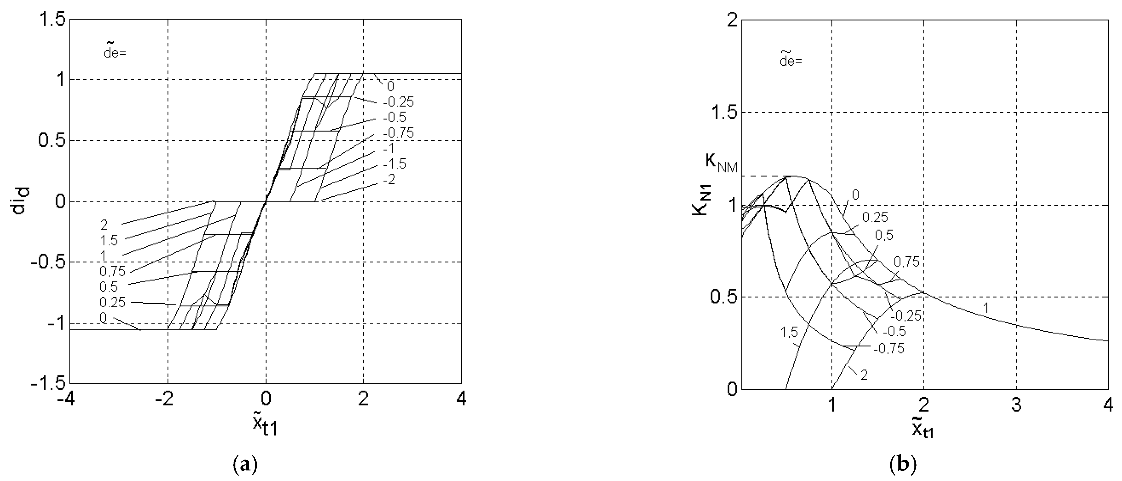
The family of characteristics $d{i}_d=\tilde{f}({\tilde{x}}_{t1};\widetilde{de})$ has the property that it is only in quadrants I and III. Figure 8a shows the family of characteristics $d{i}_d=\tilde{f}({\tilde{x}}_{t1};\widetilde{de})$ for the fuzzy block, where ${\tilde{x}}_{t1},\widetilde{de}\in R$.

The family of characteristics $K_N({\tilde{x}}_{t1};\widetilde{de})$ induces the consideration of the relationship:

$$0\le K_N({\tilde{x}}_{t1};\widetilde{de})\le K_M$$

(24)

The family of characteristics $K_N({\tilde{x}}_{t1};\widetilde{de})$, for $\tilde{x}$_t1 ≠ 0 is presented in Figure 8b.

The non-linearity N has a spatial sector property (25) deduced from (20):

$$f_N(\tilde{e},\widetilde{de})\{f_N(\tilde{e},\widetilde{de})-K_{NM}[1\hspace{1em}1]{[\tilde{e}\hspace{1em}\widetilde{de}]}^T\}\le 0,\hspace{1em}\forall [\tilde{e}\hspace{1em}\widetilde{de}]\in R^2$$

(25)

With Equation (25) the non-linearity may be seen with two inputs and one output. The theory for multivariable non-linearities from [26] may be applied. Using Equations (21)–(23), the equivalent block diagram of the system can be drawn up, as shown in Figure 9.

From the analysis of the family of characteristics in Figure 8a, it is observed that portions of characteristics of the non-linearity N with zero intervention (non-intervention) appear again, due to the limiting elements with saturation from the inputs: di_d is 0 for ${\tilde{x}}_{t1}\in [-1,\hspace{1em}1]$, for $\left|\widetilde{de}\right|=1;\hspace{1em}1,5;\hspace{1em}2$ at the limits of the universe of discourse.

To determine a Lyapunov function on the basis of which to prove the absolute internal stability of the nonlinear control system, according [24,26,27], the non-linearity ${\tilde{f}}_{\tilde{N}}(\tilde{e};\widetilde{de})$ or with the equivalent notation ${\tilde{f}}_{\tilde{N}}(\tilde{y})$ can be time-variant or invariant, but it must be continuous in time intervals and must locally satisfy Lipschitz’s property with respect to $\tilde{y}$, i.e., there must be a finite ν > 0 such that:

$$\Vert {\tilde{f}}_{\tilde{N}}({\tilde{y}}_1)-{\tilde{f}}_{\tilde{N}}({\tilde{y}}_2)\Vert \le \nu \Vert {\tilde{y}}_1-{\tilde{y}}_2\Vert , \forall {\tilde{y}}_1=[\begin{array}{cc}{\tilde{e}}_1& {\widetilde{de}}_1\end{array}] and {\tilde{y}}_2=[\begin{array}{cc}{\tilde{e}}_2& {\widetilde{de}}_2\end{array}]$$

(26)

In this case the non-linearity, ${\tilde{f}}_{\tilde{N}}(\tilde{y})$ is not time variant. The output values depend at any time only on the values at its two inputs $\tilde{e}$ and $\widetilde{de}$.

$\tilde{N}$ satisfies a condition of space sector:

$${\tilde{f}}_{\tilde{N}}(\tilde{e},\widetilde{de})[{\tilde{f}}_{\tilde{N}}(\tilde{e},\widetilde{de})-K_{\max }\left[\begin{array}{cc}1& 1\end{array}\right]\tilde{y}]\le 0, \forall t\ge 0, \forall \tilde{y}\in R^2$$

(27)

and

$$K_{\max }=c_{di}{K}_M>0$$

(28)

2.6. The Steady State of the System

It will be shown below that the steady state of the fuzzy control system considered in Figure 4, Figure 6 and Figure 9 is the only equilibrium state of the system for null entries. For this purpose, the unforced system are described by Equations (11)–(14), in which, on the one hand they are replaced ${\Omega }^{*}=0$ and $M_s=0$, and on the other hand, it is considered that the system is in steady state. It is observed that $\widetilde{de}=de=0$. Additionally, it follows from Equation (11) that ${\widetilde{di}}_d=0$. In these conditions, the following relationship results:

$${\tilde{f}}_{\tilde{N}}(\tilde{e},0)=0$$

(29)

The dependence $d{i}_d={\tilde{f}}_e(\tilde{e}, 0)$ is bijective, and Equation (29) has a unique solution $\tilde{e}=0$.

It results that absolutely all the variables take the value zero. Therefore, the point of steady state is an equilibrium point. $\tilde{e}=0$ is the unique solution of Equation (29); therefore, it is the only equilibrium point.

Therefore, it is necessary that when de = 0, the fuzzy block to give the output of di_d = 0 only when e = 0. Analyzing the single-input–single-output characteristics di_d = f (e; de), for de = 0, we may see the condition is fulfilled when defuzzification with the center of gravity is used [17,18,19]. Fuzzy blocks that use defuzzification with the mean of maximum method, for example, do not meet this condition.

2.7. The Vague State Portrait of the Rule Base

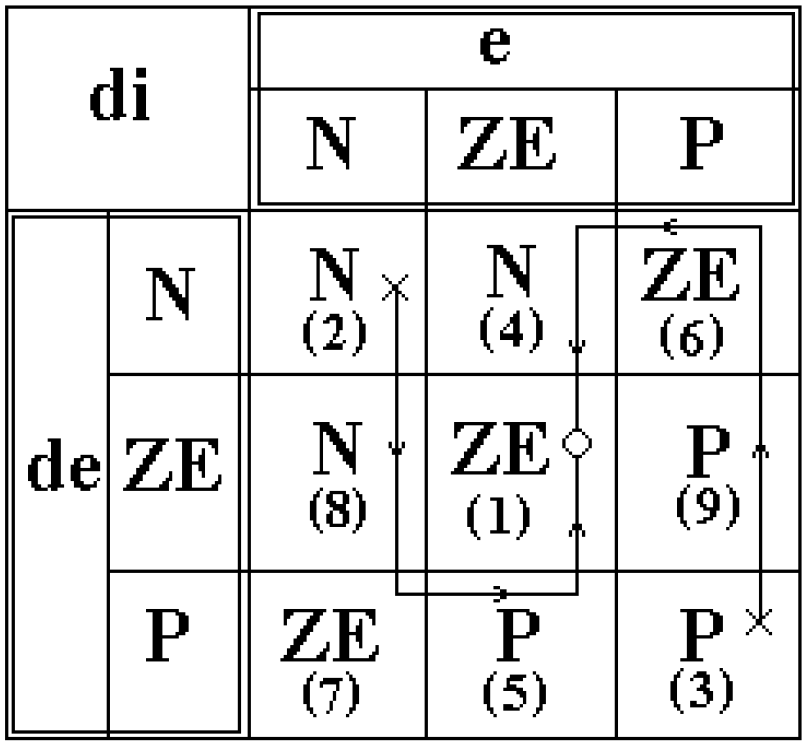
Qualitatively, a first stability analysis can be performed on the rule base chosen for the fuzzy block, in the space of vague states [28]. The rule bases may be seen as the vague state portrait. Figure 10 presents the primary rule base with 3 × 3 rules.

Thus, if it is assumed that the initial conditions are e₀ = P and de₀ = P, according to Equation (3), the command is di_d = P. If the speed control system is stable and controllable, the state path can follow the following rules in order: (9), (6), (4), with rule (1) in the steady state. If the system has initial condition specific to rules (9), (6) or (4), the specified state trajectory can only be traversed from these initial positions. Another possible route example for an ‘aperiodic linguistic behavior’ would be (2), (8), (7), (5) and (1). The rule base contains the vague state trajectories which, due to the integrative character of the controller, lead the system, from any point of the rule base from which one would start to the steady state rule. Analyzing other rule bases with 3 × 5, 5 × 5 or 5 × 7 fuzzy values [17,18,19], it is observed that they can ensure the linguistic trajectories of the fuzzy variable e, de and di_d, similar to those described above.

2.8. Observations on the Linear Part

Considering the structures of Figure 4 and Figure 9, in the situation Ω* = 0, the transfer matrix of the linear part $\tilde{L}$ is H₀(s), and $\tilde{y}(s)=H_0(s){\widetilde{di}}_{dm}(s)$. Its characteristic polynomial has a zero at the origin, due to the integrative character introduced in the dynamics of the fuzzy speed regulator, thus H₀(s) is not Hurwitz. The non-linearity ${\tilde{f}}_{\tilde{N}}(\tilde{y})$, multivariable at the input and single-variable at the output, can be assimilated with an equivalent non-linearity ${\tilde{f}}_{\tilde{N}}({\tilde{x}}_{t1};\widetilde{de})$, single-variable at the input and output. The influence of $\widetilde{de}$ makes it time-variant. The transfer function from the input variable ${\widetilde{di}}_{dm}$ to the calculation variable ${\tilde{x}}_{t1}$, which is required in connection with the block diagram in Figure 9, is obtained with the relationship:

$$H_{01}(s)=\frac{{\tilde{x}}_{t1}(s)}{{\widetilde{di}}_{dm}(s)}=\left[\begin{array}{cc}1& 1\end{array}\right]H_0(s)$$

(30)

and it has the expression:

$$H_{01}(s)=\frac{1+hs/2}{hs}{H}_i(s)\frac{k_m}{Js+k_f}{H}_{T\Omega }(s)\left(c_e+c_{de}\frac{s}{1+hs/2}\right)$$

(31)

In deducing the above expression, the equality K_CAN = 1/K_CNA was taken into account. With H_i(s), the transfer function equivalent to the current control loop was noted. H_TΩ (s) is the transfer function of the speed sensor.

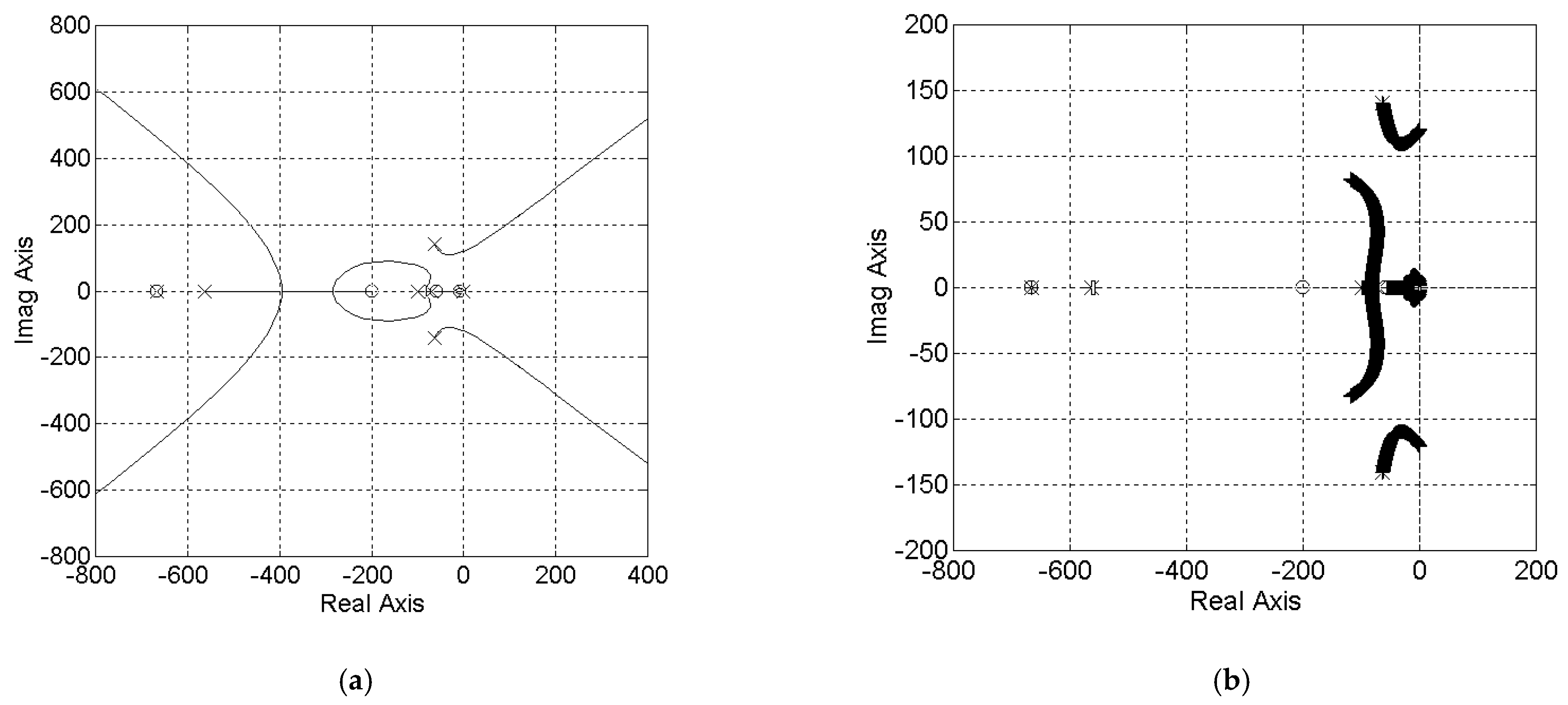
The structure from Figure 11 was used in the analysis of the possibility of stabilizing the system.

Additionally, for this structure the root locus drawn for the equation $1+K{H}_{01}(s)$ = 0, was used, which had the form of Figure 12a.

The eigenvalues of the linear part are poles: −666.67; −100; −562.66; −63.25 + 140.40 j; −63.25, −140.40 j; −69.64; −0.11; 0, and zeros: −8.51; −58.82; −666.67; −200. The root locus intersects the imaginary axis for K = K_H ≅ 4794. The detail obtained for K ∈ [0; 4795] is represented in Figure 12b. The linear part can be made stable with linear negative feedback, as shown in Figure 11. The coefficient K ∈ [ε; 4794), where ε > 0, no matter how small. This is an ε-stability situation.

In Figure 9, the nonlinear block $\tilde{N}$ must stabilize the linear part $\tilde{L}$, unstable due to the existence of the pole at the origin. According to [26], the non-linearity ${\tilde{f}}_{\tilde{N}}(\tilde{y})$ must be situated into a sector of the form [K_min, K_max], of which the sector cannot exceed the Hurwitz sector [ε, K_H):

$$[K_{\min },K_{\max }]\subset [\mathsf{\epsilon },K_H)$$

(32)

In other words, K_min must be chosen to obtain a Hurwitz matrix:

$$H_1(s)=\frac{H_{01}(s)}{1+K_{\min }{H}_{01}(s)}$$

(33)

associable with the system of Figure 11. The next section will present the solution adopted to ensure stability.

2.9. Correction of Non-Linearity Characteristics

According to [29], the relationship that characterizes the fuzzy block depends primarily on the rule base. However, the relationship $f_{BF}(e,de)$ that describes the fuzzy block also depends on the form of the chosen membership functions. The characteristics of the fuzzy block, defined only on the set [−1, 1], is characteristically situated into a sector of the form [K₁, K₂], 0 < K₁ < K₂, as can be seen from Figure 7. When introducing the saturation elements with a limiting role before the fuzzy block, the resulting non-linearity $\tilde{N}$ is situated within [0, K], as seen in Figure 8a. In order to meet the sector condition of the shape (32) necessary to ensure stability, a correction of the non-linearity characteristic according to Figure 13 is made.

The correction is made with the added variable δ_di:

$${\mathsf{\delta }}_{di}=K_c[(\tilde{e}-e)+(\widetilde{de}-de)]=K_c({\tilde{x}}_{t1}-x_{t1})$$

(34)

In this case, an important observation must be made. The correction is non-linear, it is on the feedforward channel, and it does not affect the non-linear character of the fuzzy block. It only works if there are limitations to the two inputs of the fuzzy block. It does not affect the action of the fuzzy block. It removes the action of non-linearity from the area of non-intervention. The stability is assured with the coefficient Kc [26,27]. The nonlinear correction moves the characteristics di_d = f(x_t1; de), from Figure 8a, eliminating the non-intervention area, which may be seen on the x axis, with zero value for di_d when e and de are different from zero.

The coefficient K_c > 0 must be chosen for the characteristics of the non-linear part ${\tilde{N}}_c$ to be situated within a suitable sector [K_min, K_max].

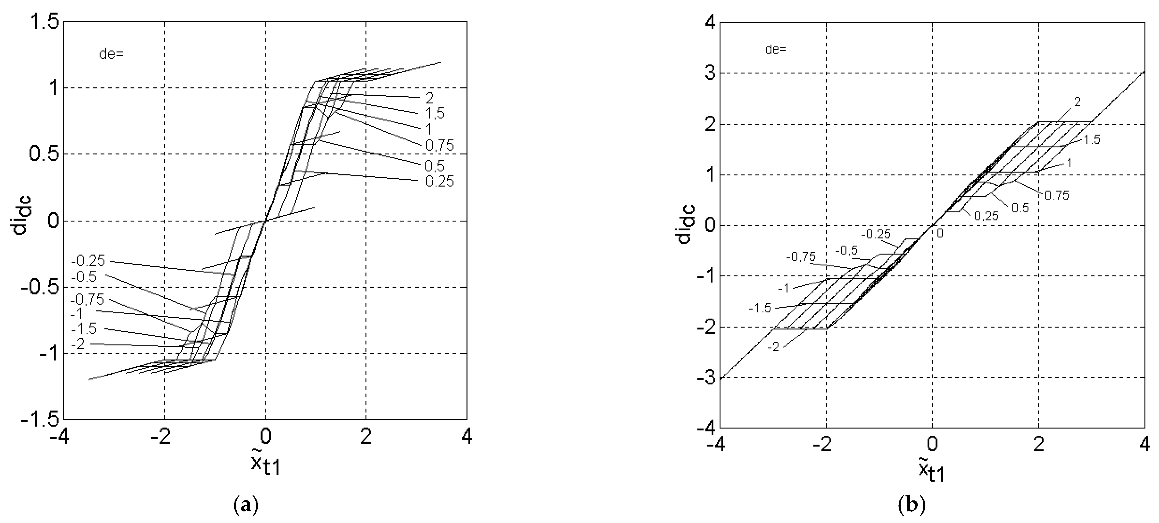
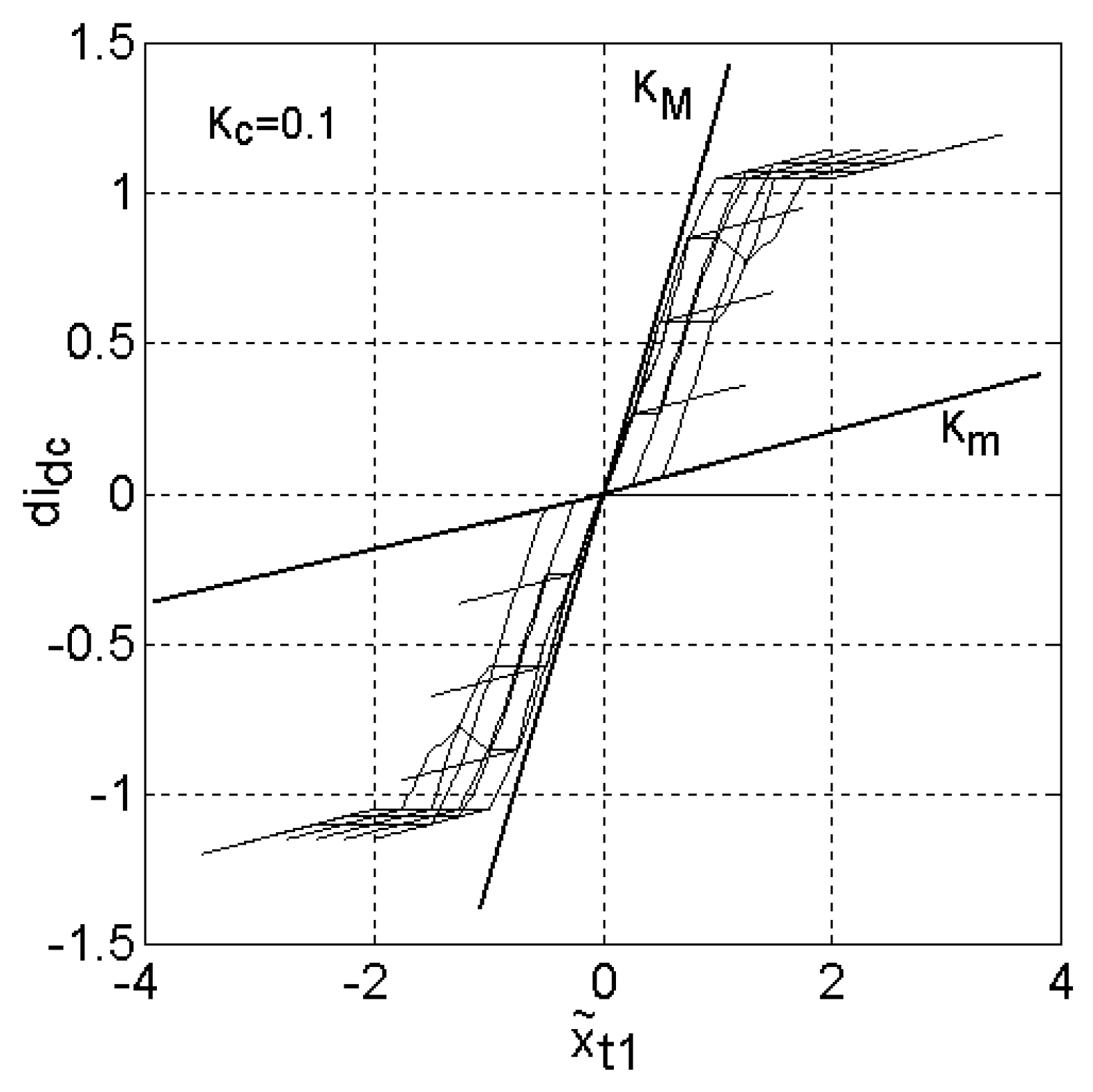
Two examples of the family of characteristics di_dc = f(${\tilde{x}}_{t1}$; $\widetilde{de}$), for K_c = 0.1 and K_c = 1, are presented in Figure 14a,b, respectively. This shows the placement in quadrants I and III and a sector condition of the form:

$$[f_{\tilde{N}}(\tilde{e},\widetilde{de})-K_m\left[\begin{array}{cc}1& 1\end{array}\right]\tilde{y}][f_{\tilde{N}}(\tilde{e},\widetilde{de})-K_M\left[\begin{array}{cc}1& 1\end{array}\right]\tilde{y})]\le 0,\forall y\in R^2$$

(35)

This condition can be transcribed as:

$$(d{i}_{dc}-K_m{\tilde{x}}_{t1})(d{i}_{dc}-K_M{\tilde{x}}_{t1})\le 0, \forall {\tilde{x}}_{t1}\in R$$

(36)

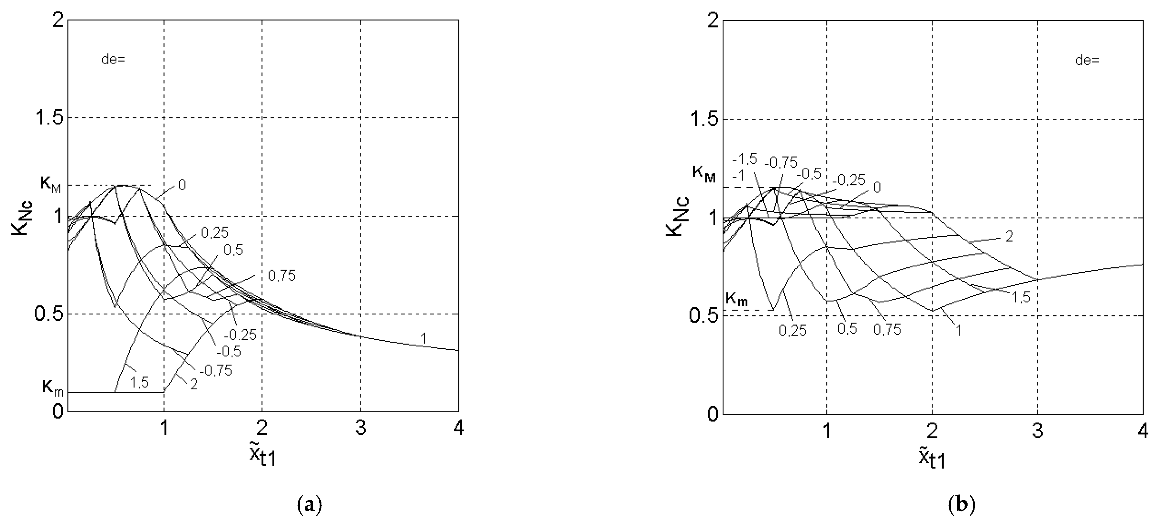
In order to determine K_m and K_M, the families of characteristics are considered:

$$K_{Nc}({\tilde{x}}_{t1}; \widetilde{de})=\frac{d{i}_{dc}}{{\tilde{x}}_{t1}},\hspace{1em}{\tilde{x}}_{t1}\ne 0$$

(37)

from Figure 15, associated with the features of Figure 14.

It can be observed that the family of characteristics K_Nc($\tilde{x}$_t1; $\widetilde{de}$), has the limits K_m and K_M of the sector in which it is situated, variable depending on the coefficient K_c.

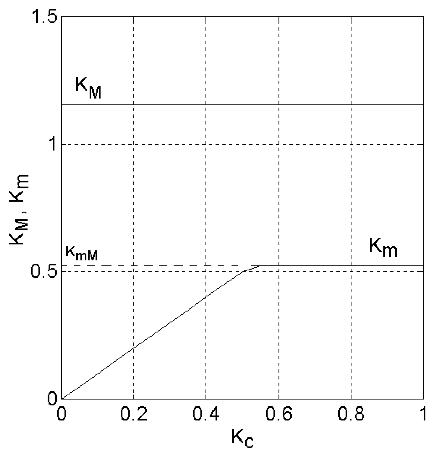
Figure 16 shows how these two limits vary depending on the value of $K_c\in \left[0, 1\right]$.

Analyzing Figure 16, it can be seen that the value of K_M is constant, being approximately 1.17, for any K_c. Therefore, the correction does not change the maximum associated with the family of functions K_Nc($\tilde{x}$_t1; $\widetilde{de}$). The value of K_m varies linearly with K_c, from 0 to K_mM ≅ 0.52, for K_c = 0.55. K_m is constant at about 0.52 for K_c values greater than 0.55. The ratio between K_m and K_M varies depending on K_c between 0 and about 0.32. Corroborating this result with condition (32), it follows that c_di and K_c must be adopted so that:

$$[c_{di}{K}_m,c_{di}{K}_M]\subset [K_{\min },K_{\max }]\subset [\mathsf{\epsilon },K_H)$$

(38)

As can be seen from the developed equivalent block diagrams, the c_di current increment coefficient is included in the non-linearity structure. It simultaneously affects both limits of the sector in which the non-linearity ${\tilde{N}}_c$ falls, according to Equation (38). The lower limit of the sector in which the non-linearity ${\tilde{N}}_c$ falls is also corrected with the help of the correction coefficient K_c. The accessible values of K_min, K_max and c_di for the speed control system of the DC machine will be determined following a stability analysis.

3. Stability Analysis

3.1. Internal Stability Analysis

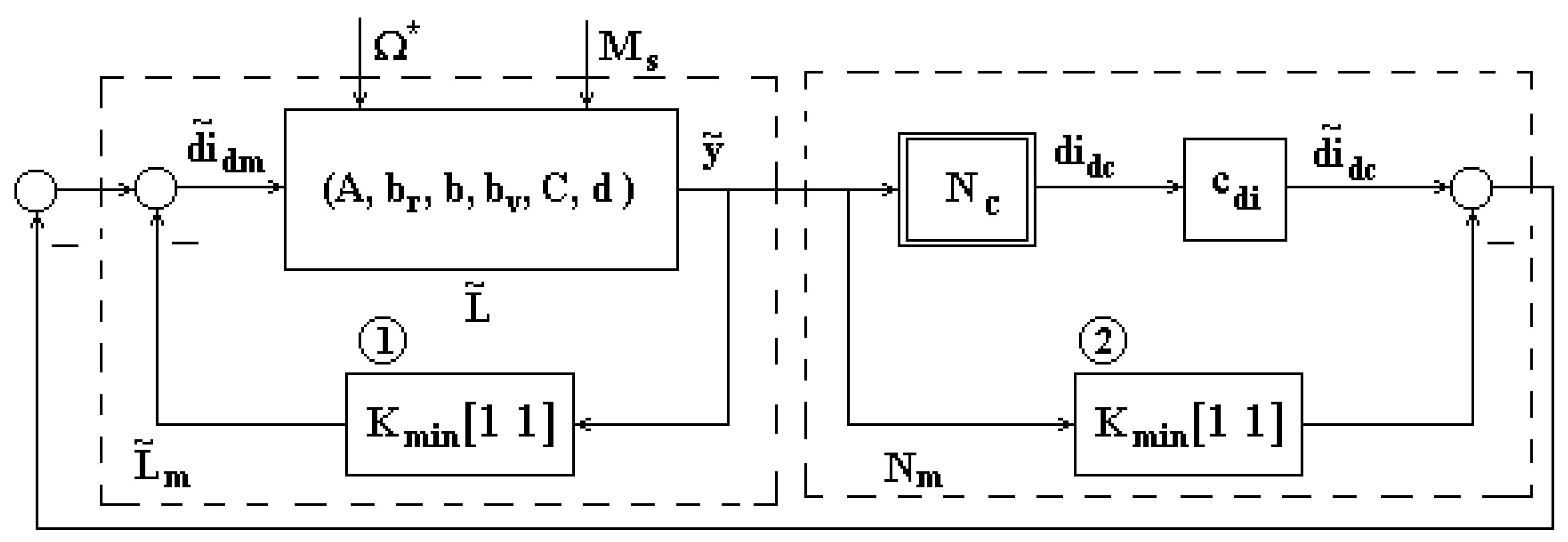
In order to analyze the stability of the DC motor fuzzy speed regulation system, a fictitious transformation of the control loop of Figure 13, shown in Figure 17 [26,27], is used.

A negative feedback (block 1) $K_{\min }[1\hspace{1em}1]$ is applied to the linear part, and also for its total compensation on the non-linear part (block 2). The result is a modified linear part ${\tilde{L}}_m$ and a non-linear part N_m. The linear part $\tilde{L}$ has the non-Hurwitz state matrix A, and the non-linear part ${\tilde{f}}_{\tilde{N}}(\tilde{y})$ satisfies:

$$[{\tilde{f}}_{\tilde{N}}(\tilde{y})-K_m\left[\begin{array}{cc}1& 1\end{array}\right]\tilde{y}][{\tilde{f}}_{\tilde{N}}(\tilde{y})-K_M\left[\begin{array}{cc}1& 1\end{array}\right]\tilde{y})]\le 0, \forall \tilde{y}\in R^2$$

(39)

The linear part ${\tilde{L}}_m$ has the mathematical model:

$$\begin{array}{l}\dot{x}=(A-b_r{K}_{\min }\left[\begin{array}{cc}1& 1\end{array}\right]C)x+b_r·{\widetilde{di}}_{dm}+b{\Omega }^{*}+b_v{M}_s\\ \tilde{y}=Cx+d·{\Omega }^{*}\end{array}$$

(40)

Let K_min be such that the matrix of the system ${\tilde{L}}_m$

$$\tilde{A}=A-b_r{K}_{\min }\left[\begin{array}{cc}1& 1\end{array}\right]C$$

(41)

is Hurwitz. Then, the nonlinear part N_m has the relationship:

$$f_m(\tilde{y})={\tilde{f}}_{\tilde{N}}(\tilde{y})-K_{\min }\left[\begin{array}{cc}1& 1\end{array}\right]\tilde{y}$$

(42)

It can be clearly seen that from Equation (39) this results in:

$$f_m(\tilde{y})[f_m(\tilde{y})-K\left[\begin{array}{cc}1& 1\end{array}\right]\tilde{y})]\le 0, \forall \tilde{y}\in R^2$$

(43)

with K = K_max − K_min.

For the analysis of the internal stability the unforced (autonomous) system was considered, in which Ω* = 0 and M_s = 0. The mathematical model of the unforced system is:

$$\begin{array}{l}\dot{x}=\tilde{A}x+b_r{\widetilde{di}}_{dm}\\ \tilde{y}=Cx\\ {\widetilde{di}}_{dm}=-f_m(\tilde{y})\end{array}$$

(44)

The system (Equation (44)) has a non-linearity with two input variables and one output variable. In [26], it is recommended to use the circle criterion for multivariable systems in which the non-linearity has an equal number of inputs and outputs. That is not the case here. Using the change of non-linearity made in the paper from the form with two input variables (20) to the form with a single input variable and a parameter ((21) ÷ (23)), the circle criterion proposed in [24,26,27] can be used, for systems with a single input–single output non-linearity, but time-variant. Furthermore, it will be shown that a statement of the circle criterion can be given even if the non-linearity has two input variables and only one output variable, but satisfies Equation (38). The demonstration occurs in three stages.

Stage I. In the first stage, the following particular variant of the Kalman–Yakubovich–Popov lemma [24,25,26,27] may be used:

Lemma 1.

Let it be:

$$F(s)=1+K{H}_1(s)=1+K\left[\begin{array}{cc}1& 1\end{array}\right]C{(sI-\tilde{A})}^{-1}{b}_r$$

(45)

with H₁(s) defined by (33),$\tilde{A}$is a Hurwitz matrix,$(\tilde{A},b_r)$controllable and$([1\hspace{1em}1]C,\tilde{A})$observable. Then, F(s) is strictly positive if and only if there is a positively defined symmetric matrix P with (P = P^T > 0), a vector M and a constant ε > 0 such that:

$$\begin{array}{l}P\tilde{A}+{\tilde{A}}^{T}P=-M^{T}M-\mathsf{\epsilon }P\\ P{b}_r=C^{T}K{\left[\begin{array}{cc}1& 1\end{array}\right]}^T-\sqrt{2}{M}^T\end{array}$$

(46)

Taking into account Equations (31) and (33), this results in:

$$F(s)=1+(K_{\max }-K_{\min })\frac{H_{01}(s)}{1+K_{\min }{H}_{01}(s)}=\frac{1+K_{\max }{H}_{01}(s)}{1+K_{\min }{H}_{01}(s)}=\frac{1+K_{\max }\left[\begin{array}{cc}1& 1\end{array}\right]H_0(s)}{1+K_{\min }\left[\begin{array}{cc}1& 1\end{array}\right]H_0(s)}$$

(47)

Stage II. It is assumed that the conditions in the Kalman–Yakubovich–Popov lemma are met and there are matrices P and M. Then, with the matrices P and M, a Lyapunov function V(x) is constructed, and it is proved that its derivative $\dot{V}(x)$ is negative when the sector condition is fulfilled [30].

Thus, the Lyapunov function is chosen:

$$V(x)=x^{T}Px$$

(48)

where $x=x(t)$ is given by Equation (44).

Consequently:

$$\dot{V}(x)=x^T(P\tilde{A}+{\tilde{A}}^{T}P)x-2x^{T}P{b}_r{f}_m(\tilde{y})$$

(49)

Increasing the right parameter of Equation (49) by $-2f_m(\tilde{y})(f_m(\tilde{y})-K\left[\begin{array}{cc}1& 1\end{array}\right]\tilde{y})\ge 0$, see (43), we obtain:

$$\begin{array}{l}\dot{V}(x)\le x^T(P\tilde{A}+{\tilde{A}}^{T}P)x-2x^{T}P{b}_r{f}_m(\tilde{y})-2f_m(\tilde{y})\{f_m(\tilde{y})-K\left[\begin{array}{cc}1& 1\end{array}\right]\tilde{y}\}\\ =x^T(P\tilde{A}+{\tilde{A}}^{T}P)x-2x^{T}P{b}_r{f}_m(\tilde{y})-2f_m(\tilde{y})\{f_m(\tilde{y})-K\left[\begin{array}{cc}1& 1\end{array}\right]Cx\}\\ = x^T(P\tilde{A}+{\tilde{A}}^{T}P)x+2x^T(C^{T}K{\left[\begin{array}{cc}1& 1\end{array}\right]}^T-P{b}_r)f_m(\tilde{y})-2f_m^2(\tilde{y})\end{array}$$

(50)

Making substitutions in the right member of the Equation (50) in the first and second term based on Equation (46), using the matrices P and M and the number ε, results in:

$$\begin{array}{l}\dot{V}(x)\le x^T(-M^{T}M-\mathsf{\epsilon }P)x+2\sqrt{2}{x}^T{M}^T{f}_m(\tilde{y})-2f_m^2(\tilde{y})\\ =-\mathsf{\epsilon }{x}^{T}Px-x^T{M}^{T}Mx+2\sqrt{2}{x}^T{M}^T{f}_m(\tilde{y})-2{\tilde{f}}_m^2(\tilde{y})\\ =-\mathsf{\epsilon }{x}^{T}Px-{[Mx-\sqrt{2}{f}_m(\tilde{y})]}^T[Mx-\sqrt{2}{f}_m(\tilde{y})] \le -\mathsf{\epsilon }{x}^{T}Px\end{array}$$

(51)

Therefore, the existence of P, M and ε that satisfy (46) makes $\dot{V}(x)$ negative. Consequence. Consider the system (44), where $\tilde{A}$ is Hurwitz, ($\tilde{A}$, b_r) is stabilizable and f_m($\tilde{y}$) satisfies the sector conditions (42) and (43) on R³. Then, the system (44) is globally absolutely stable if the transfer function F(s), given by (45) and (47), is strictly positive real.

Stage III. After the above demonstration, it can be stated that the following statement for the circle criterion is valid, if the non-linearity has two input variables and one output variable:

Theorem 1 (Circle criterion).

It is considered that the non-linear system with the linear part ε-stable, is controllable and observable, with the transfer function H₀₁(s) and the non-linearity of the fuzzy block satisfying the sector condition (39). The system is globally absolutely stable if H₁(s) is Hurwitz and F(s) is strictly positive real.

The transfer matrix H₀(s) is a transfer matrix of a linear part with one input variable and two output variables.

In these conditions, the system is absolutely stable in the sector [K_min, K_max] if the hodograph H₁(jω) is located to the right of a vertical line passing through the point of abscissa (−1/K, 0), with K ≥ K_max−K_min. A stability analysis based on a graphical method is performed in [31], but for a fuzzy controller with two inputs and two outputs.

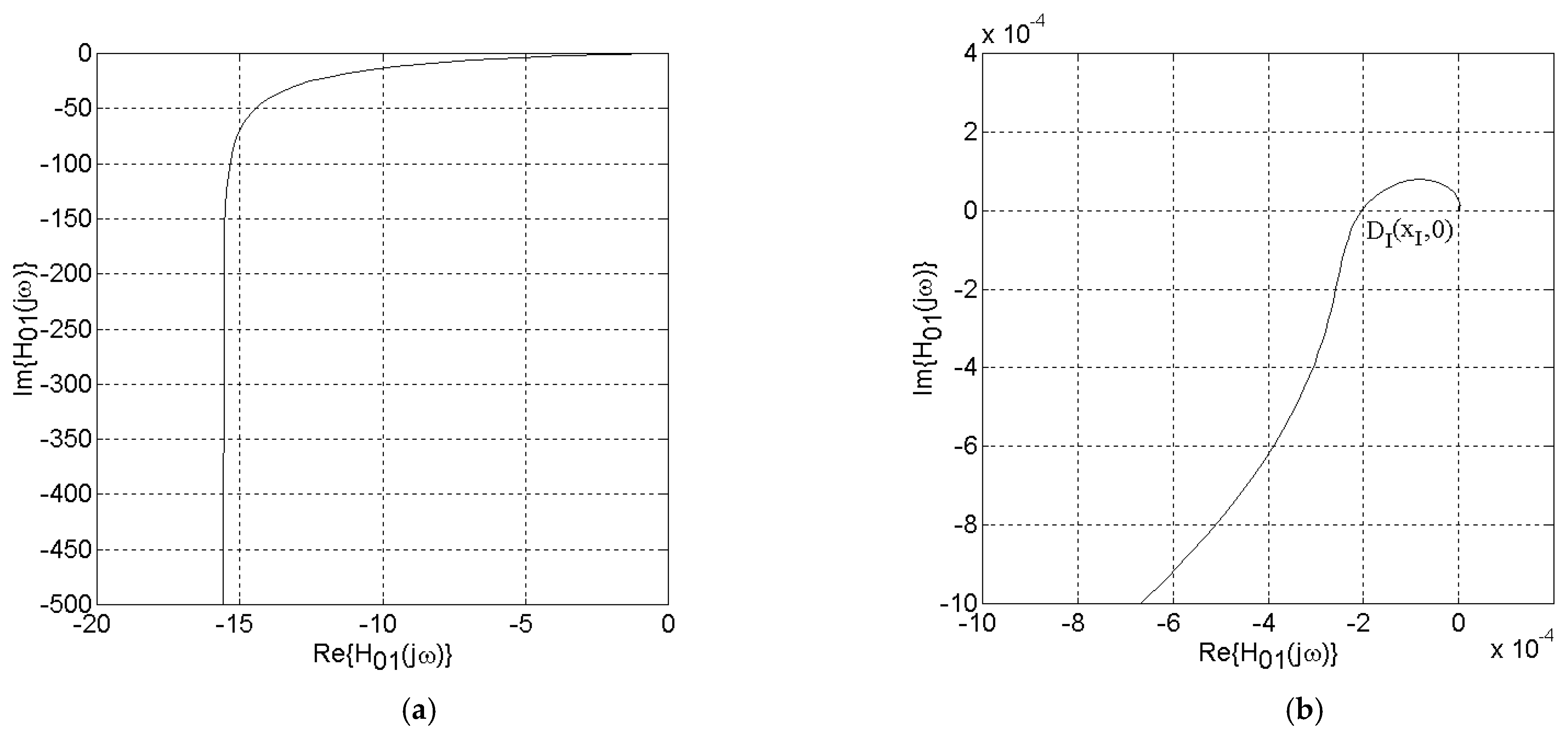
To use the circle criterion, the hodograph of the linear part H₀₁(jω) is drawn, which has the shape of Figure 18a, with detail shown in Figure 18b.

The hodograph of the linear part H₀₁(jω) imposes a dependence between K_max and K_min. The circles must be to the left and most tangent to the hodograph. If there is no correction, the non-linear part remains in the sector [0, K] and we cannot tell from the equilibrium point x = 0 whether it is stable or unstable. There are states of the system with V(x) > 0 and $\dot{V}(x)\ge 0$, but we do not know whether or not the system passes to states in which V(x) > 0 and $\dot{V}(x)<0$.

3.2. Determining the Limits of the Stability Sector

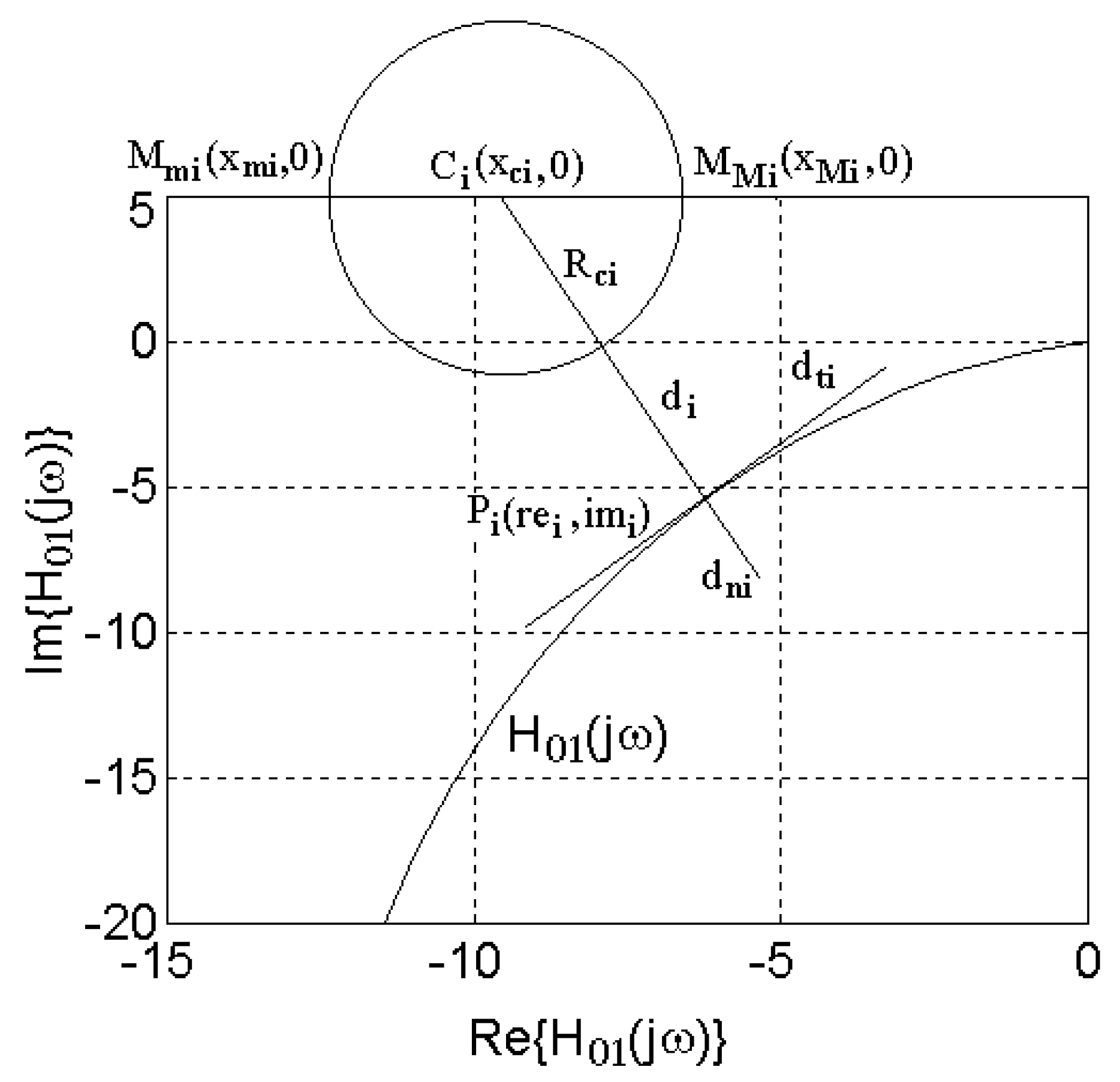
In Figure 18b, it is observed that the hodograph intersects the real axis at the point D_I, of coordinates x_I ≅ −1/2500 and y_I = 0. Analysis of the properties of the sector is conducted for Re{H(jω)} ≤ x_I, to ensure that the stability the circles would be located to the left of the point D_I. To ensure stability, the circles must have a radius R_c less than the distance d from their center to the hodograph. The analysis is made with reference to Figure 19.

For a certain frequency ω_i, i = 1, …, n_p there is determined by calculations a point on the hodograph denoted P_i, of coordinates (u_i, v_i). At this point, the hodograph admits a tangent denoted d_ti and a normal denoted d_ni. The distance from the center C_i of a circle that can be built to the left of the hodograph is calculated on the normal d_ni to the hodograph. It is the distance between the point on the hodograph P_i at which the normal d_ni rises and the point C_i at which the normal intersects the real axis. If circles are constructed on the real axis with center in x_ci, these circles must have radius R_ci less than the distance d_i. Circles that can be constructed with the center in x_ci intersect the real axis to the left at the point M_m of coordinates y_m = 0 and,

$$x_{mi}=-1/K_{\min i}$$

(52)

and to the right at the point M_M of coordinates y_M = 0 and,

$$x_{Mi}=-1/K_{\max i}$$

(53)

The extreme values of the x_mi and x_Mi coordinates are limited by the distance d_i to the hodograph:

$$\begin{array}{l}{(x_{mi})}_{\min }=x_{ci}-d_i\\ {(x_{Mi})}_{\max }=x_{ci}+d_i\end{array}$$

(54)

Additionally, the values of the extreme limits of the sector are limited:

$$\begin{array}{l}{(K_{\min i})}_{\min }=-1/{(x_{mi})}_{\min }\\ {(K_{\max i})}_{\max }=-1/{(x_{Mi})}_{\max }\end{array}$$

(55)

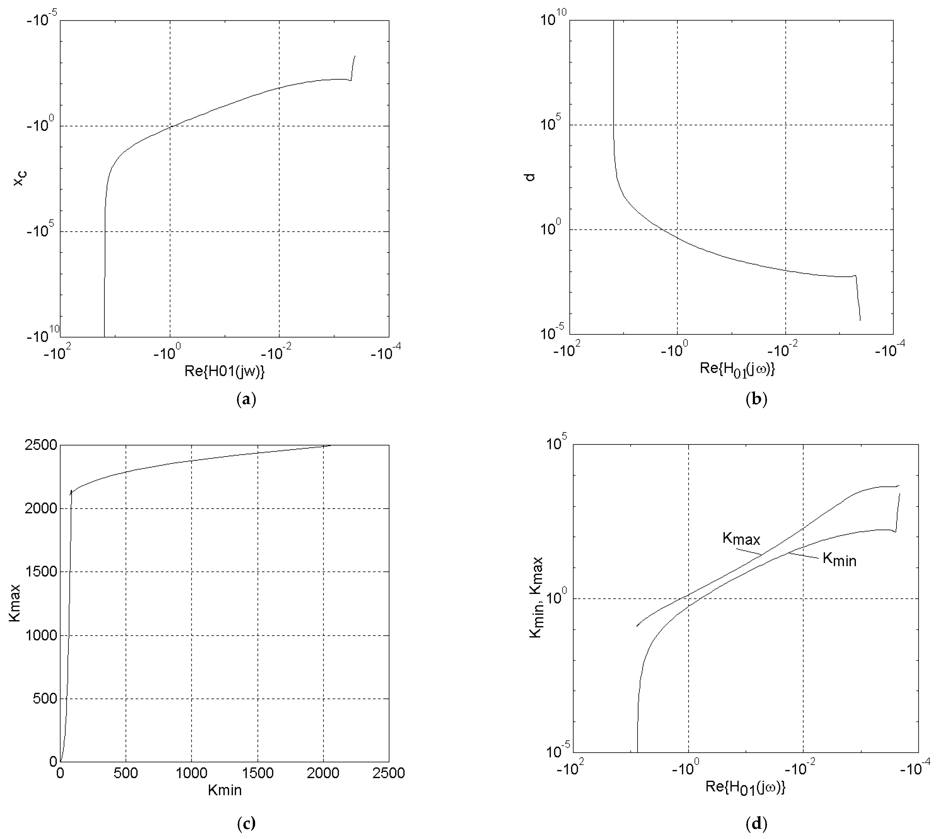
Below are the graphs of the dependencies between the parameters that characterize the location of the circles relative to the hodograph.

Figure 20a shows how the abscissa x_c of the center of the circle varies, located on the normal taken at a point on the hodograph. The point on the hodograph is defined by the value of the real coordinate Re{H₀₁(jω)}. It is natural that as the position on the hodograph moves to the left, the position of the center of the circle must move to the left. On the central part of the characteristic, the dependence is almost linear. In the vicinity of the intersection of the hodograph with the real axis, there is a portion on which there is a wider margin of location of the center of the circle. To the left of the hodograph asymptote, the center of the circle can be located as far to the left as the real axis. This figure shows that the dependence between the position on the hodograph and the center of the circle is univocal, i.e., from a point on the real axis, only one normal can be taken to the hodograph. Figure 20b shows how the distance from the center of the circle varies from normal to hodograph, depending on the position of a point on the hodograph. Figure 20c shows the dependence between the extreme values of K_max and K_min. This feature is plotted parametrically, depending on the position on the hodograph. Figure 20d shows how K_max and K_min depend on the abscissa Re{H₀₁(jω)} of the tangent point of the circle at the hodograph.

It is observed, as is natural, that for points on the hodograph located closer to the D_I point (from Figure 18b), the maximum limit of the stability sector increases, tending to the Hurwitz value, the maximum limit of the sector K_H = 2500. It is observed that the K_max/K_min ratio has the maximum value, of approximately 12, next to the point of intersection with the real axis. The ratio decreases in the central area of the hodograph. The ratio obviously increases to the left of the asymptote at the hodograph. The constraint imposed by the non-linear part depends on K_c, as shown in Figure 16 and the value of the current increment coefficient c_di. A maximum c_diM value can be determined for the current increment coefficient. The maximum c_diM value is limited by the capability of the speed control system to control the motor supply current. It is determined by the maximum numerical value of the prescribed current:

$$c_{diM}=I_M{K}_{CAN}{K}_{Ti}$$

(56)

K_max is given by the product c_di.K_M. The maximum value of K_M is constant, and at the same time, it depends on K_c. Additionally, K_mM varies with K_c.

The maximum range in which a stability sector can be chosen is determined using Figure 21.

In this figure, the characteristics are represented in logarithmic coordinates, to highlight the various portions of it. The values of c_di can also be placed on the abscissa axis (see the upper side), because:

$$c_{di}=K_{\max }/K_M$$

(57)

Additionally, in Figure 21, the characteristic:

$$K_{\min M}=c_{di}{K}_{mM}$$

(58)

is drawn in which K_mM (see Figure 16) depends on K_M. The value of K_minM increases as K_c increases.

The stability sector can be chosen only in the field shaded in the figure, because only these domains are located between the graph of K_min = f(K_max) and the graph of K_minM = f(c_di).

The domain is limited to:

$$K_{\max M}=c_{diM}{K}_M$$

(59)

The verification of the findings regarding the stability domains is presented in the paper by transient regime analyses of the unforced system.

3.3. Indications for Correction Characteristics of Non-Linearity and Determination of the Stability Sector

To establish an acceptable dynamic behavior for the closed loop control system, the values of the scaling coefficients c_e, c_de and c_di may be chosen. Additionally, to correct the non-linearity characteristics, the value of the coefficient K_c may be modified. Below are some indications for choosing the parameters c_di and K_c, considering the previously chosen values of the parameters c_e and c_de, for the case of the electric drive taken as an example in the paper.

(1) For a certain type of fuzzy block, the values K_m and K_M may be chosen from the characteristics K_Nc = f($\tilde{x}$_t1), or di_dc = f($\tilde{x}$_t1; de).

(2) The current incremental coefficient is limited by the capability of the control system to regulate the current through the electric machine. The prescribed current difference at a sampling step h is:

$$\Delta i_{nk+1}^{*}=i_{nk+1}^{*}-i_{nk}^{*}$$

(60)

The current increment coefficient can be determined with the relationship that describes the numerical integration function:

$$c_{di}=\frac{\Delta i_{nk+1}^{*}}{d{i}_{dk+1}}$$

(61)

For the example taken in consideration, the maximum value of the prescribed current may not exceed: $I_M^{*}=K_{CAN}{I}_{aM}{K}_{Ti}=204.8\times 10.8=2211.84$. This value is dimensionless. It only appears in calculations. The maximum value at the fuzzy block output is approximately $d{i}_{dM}=1.4$. Therefore, at an integration step, on a sampling period h, a value greater than $c_{diM}=I_M^{*}/d{i}_{dM}\cong 1579.89$ is not justified for the current coefficient. For this maximum value of the current increment coefficient, a maximum value of the upper limit of the non-linearity of c_diM.K_M = 1848.47 can be chosen.

(3) The values of the coefficients c_di and K_c are chosen so that $K_{\min }\le c_{di}{K}_m<c_{di}{K}_M\le K_{\max }<K_H=4794$.

In practice, this choice will be made following repeated transient regime analyses, establishing a value of c_di that will ensure an acceptable dynamic behavior.

(4) In choosing c_di, the maximum value K_M of the upper limit of non-linearity for a certain fuzzy block must be taken into account. For a fuzzy block with 3 × 3 fuzzy variables, max–min inference and defuzzification with center of gravity, with transfer characteristics from Figure 3, K_M = 1.17, and results in:

$$c_{di}=K_{\max }/K_M$$

(62)

This value must be less than c_diM.

(5) K_c is chosen with the relationship:

$$K_c=r_k{K}_M$$

(63)

where the ratio,

r_K = K_min/K_max

(64)

is taken into account.

If K_c results in relatively small values, the non-linearity of the fuzzy block does not change significantly. The non-linear character of the fuzzy block, the main attribute of the fuzzy controller, remains.

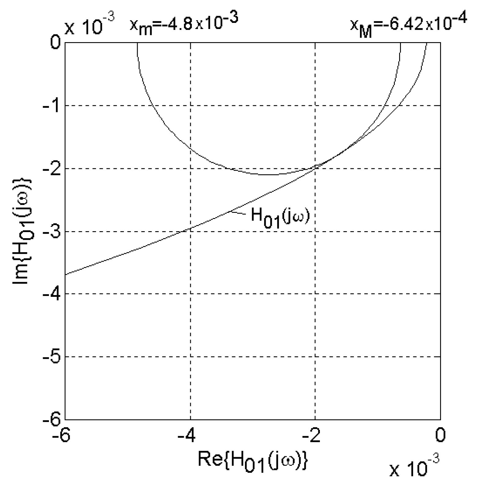
It is recommended that the family of characteristics f_Nc($\tilde{x}$_t1; $\widetilde{de}$) be included in the stability sector; therefore, at variations of the parameters of the electric drives, these characteristics do not leave the stability sector.

The placement of a circle with the following coordinates: x_m = −0.0048 and x_M = −6.416 × 10⁻⁴, close to −1/K_H, is shown in Figure 22.

In this case, the limits of the stability sector are: K_min = 206.26 and K_max = 1558.4. The center of the circle has the abscissa x_c = −0.0027. The distance from the center to the hodograph has the value d = 0.0021. The tangent of the circle at the hodograph has the coordinates (−0.0016; −0.0017). The ratio between the extreme values of the sector limits has the value r_K = 7.5553. For this circle, c_di ≅ 1332 and K_c ≅ 0.1 may be approximated.

Figure 23 presents an example of the location of the characteristics di_dc($\tilde{x}$_t1; $\widetilde{de}$) in quadrants I and III, in the sector [K_m, K_M] admitted.

3.4. Testing the Domain of Stability Sector Limits

Verification of the findings made in the previous paragraphs regarding the internal stability was performed for some cases specific to the domain in which the correction parameters of the non-linearity K_c and c_di can take values. This verification consisted of performing transient analyses on the model in Figure 1, in which the speed controller was numerically implemented. The unforced regime was taken into account, because it was considered when the internal stability analysis was performed. The values chosen for the correction parameters are presented in

Table 1. Stability verification cases.

Case	cdi	Kc
1	1500	0.1
2	100	0.55
3	10	0.55
4	1	0.55
5	5000	0.55

.

The values chosen for c_di place the non-linearity in various parts of the stability domain, as in Figure 21.

Following the correction made on the non-linearity, the PI fuzzy speed controller has the block diagram shown in Figure 24 [13,14,26,27].

It is observed that the correction performed resulted in a quasi-fuzzy structure, in which a linear structure was introduced in parallel with the fuzzy block.

The Matlab/Simulink program was used to simulate the fuzzy control system.

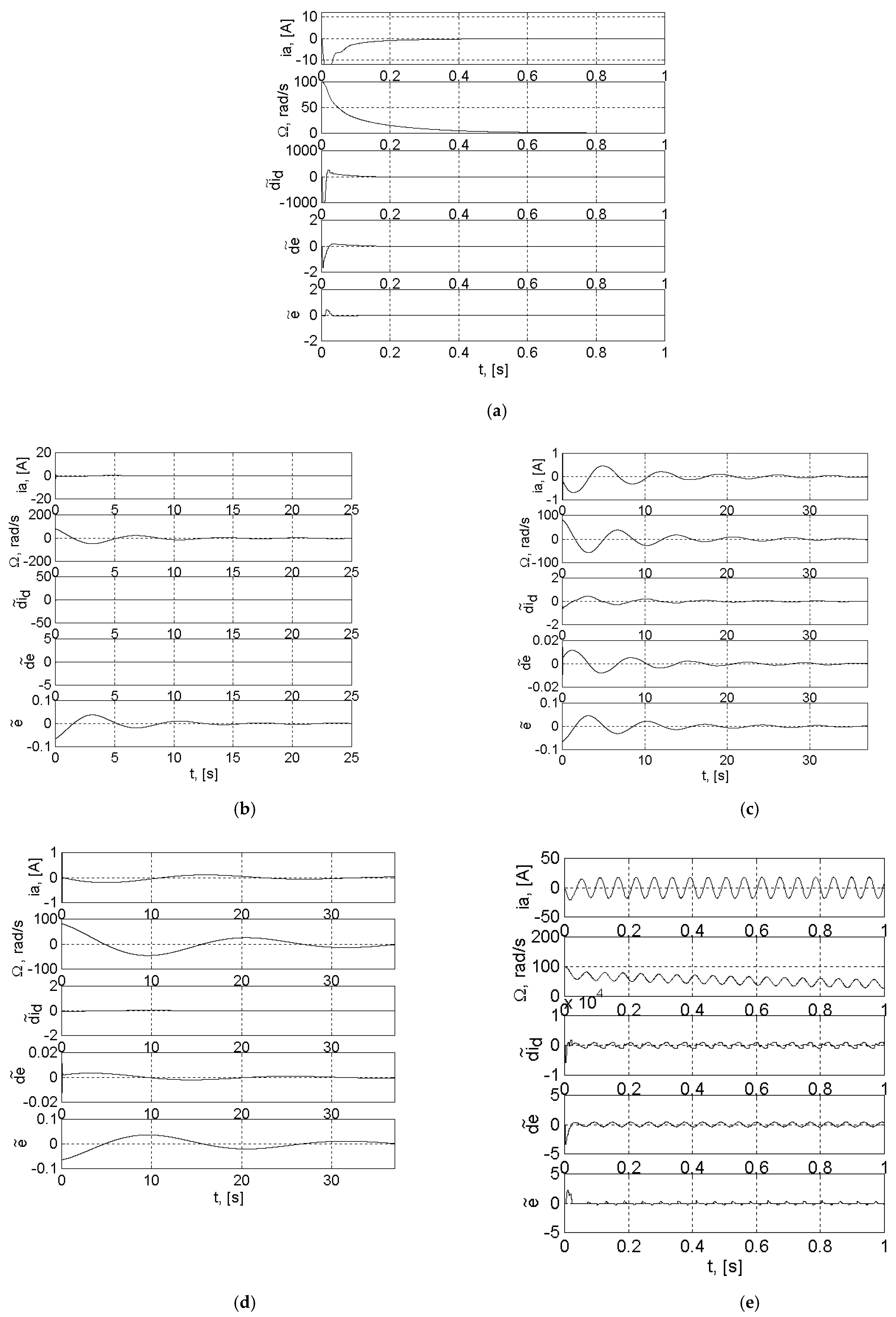
An unforced control system, with Ω* = 0 and M_s = 0, was considered. It was also considered that the control system was brought to a certain initial state, for example, i_a0 = 1 A şi Ω₀ = 100 rad/s. In the analysis of the transient regime, the behavior over time of the state variables i_a and Ω and of the variables $\tilde{e}$, $\widetilde{de}$ and ${\widetilde{di}}_d$ was analyzed. In Figure 25a–e, the characteristics in the unforced regime for the variables chosen above are presented in cases 1, 2, 3, 4 and 5 of Table 1, respectively.

It is observed that in cases 1, 2, 3 and 4, the steady state is a state of stable equilibrium, and in case 5, it is at the limit of stability, practically unstable. The f_m($\tilde{y}$) function is null outside that neighborhood. Continuing the reasoning, one can take this neighborhood no matter how small around the steady state, and then the fuzzy block can be linearized around the steady state. It follows that in this vicinity, in the stability analysis of the speed control system of the electric drive based on fuzzy regulator, criteria from the stability analysis for linear systems might be used. Moreover, the above findings could suggest that the fuzzy regulator-based control system is asymptotically internal stable even in the Hurwitz sector [0, K_H).

3.5. Input–Output Stability Analysis

For analysis of the input–output stability of the speed control system of the DC machine based on the fuzzy PI controller, the block diagram in Figure 4 and the mathematical input-state–output model given by Equations (11) and (12) considered these relations written in a general form:

$$\begin{array}{c}\dot{x}(t)=f_x(x(t),u(t))\\ \Omega (t)=f_{\Omega }(x(t),u(t))\end{array}$$

(65)

where non-linearity was considered introduced in f_x.

The input variables were:

$$u={[{\Omega }^{*}\hspace{1em}{M}_s]}^T$$

(66)

and the output variable was Ω.

In the analysis of internal stability, the emphasis was on the behavior of state variables for the unforced system. The mathematical input-state–output model connected the output Ω and the inputs, grouped in the vector of the input variables u, by means of the internal structure of the speed regulation system based on the fuzzy regulator. In the analysis of input–output stability, the system is seen as a black box, which can be accessed only through inputs and outputs.

According to the application considered, the grouped inputs in the vector of the input variables u belong, according to the theory [26], to a normed linear signal space £² of functions u:[0, +∞] → R². Such a space is, for example, the space of uniformly bounded functions £_∞, provided by the norm:

$${\Vert u\Vert }_{\infty }=\underset{t\ge 0}{\sup }\Vert u(t)\Vert <\infty$$

(67)

If u ∈ £² is considered to be a suitable input, which ‘behaves well’, the question is whether the output Ω ‘will behave well’, meaning whether Ω will belong to a function space with a similar norm as to Equation (67). A system that has the property that any input with ‘good behavior’ generates an output with ‘good behavior’ is called a stable input–output system [26]. For the case when the inputs and outputs belong to uniformly bounded function spaces, the definition of input–output stability becomes the notion of bounded input-bounded output (BIBO) stability. In other words, the system is £_∞—stable if for any bounded input, the output is bounded.

The following theorem [24,26,27] is used in the study of input–output stability.

Theorem 2.

Let the dynamic system given by the Equation (65), where x ∈ R⁸, u ∈ R², Ω ∈ R, f_x:R⁸ × R² → R⁸ is derivable and f_Ω: R⁸ × R² → R is continuous. Suppose that:

1. 

x = 0 is an equilibrium point of (65) with u = 0, i.e., f_x(0, 0) = 0, ∀t ≥ 0;

2. 

x = 0 is an equilibrium point global exponential stable of the autonomous (unforced) system:

$$\dot{x}=f_x(x,0)$$

(68)

3. 

The Jacobian matrix $\left[\partial f_x/\partial x\right]$, evaluated for u = 0 and$\left[\partial f_x/\partial u\right]$are globally bounded;

4. 

f_Ω(t, x, u) satisfies:

$$\Vert f_{\Omega }(x,u)\Vert \le k_1\Vert x\Vert +k_2\Vert u\Vert +k_3$$

(69)

globally, for k₁, k₂, k₃ > 0.

Then, for any $\Vert x(0)\Vert \le \eta$, there exist the constants γ > 0 and$\beta =\beta (\eta ,k_3)\ge 0$such that

$$\underset{t\ge 0}{\sup }\Vert \Omega (t)\Vert \le \underset{t\ge 0}{\sup }\Vert u(t)\Vert +\beta$$

(70)

• Condition 1 is met, as shown in Section 3.1;
• For condition 2, the following theorem [26] can be taken into account.

Theorem 3.

Let x = 0 be a point of equilibrium of the nonlinear system, where f_x is derivable with respect to the state variables and the Jacobian matrix$\left[\partial f_x/\partial x\right]$is bounded and Lipschitz. Thus,

$${\tilde{A}}_0={\frac{\partial f_x}{\partial x}|}_{x=0}$$

(71)

Then, the origin is a stable exponential equilibrium point for the control system, if it is a stable exponential equilibrium point for the linear system:

$$\dot{x}={\tilde{A}}_{0}x$$

(72)

The matrix${\tilde{A}}_0$in this case is given by the relationship:

$${\tilde{A}}_0=A-b_r(c_{di}{K}_0)\left[\begin{array}{cc}1& 1\end{array}\right]C$$

(73)

where

$$K_0=K_{BF}(0;0)$$

(74)

In this case, the linearized system around the origin was considered, and for the fuzzy block, the value in Equation (74) of function K_BF(x_t1; de) was considered.

The linear system is exponentially stable because all its poles have a real negative side.

• The Jacobian matrices in condition 3 have, as elements, the coefficients of the state and input variables in Equations (13) and (14), respectively, and the partial derivatives of $f_m(\tilde{e},\widetilde{de})$ in relation to the state variables and with respect to the input variables. The coefficients of the system are constant, and therefore limited. Fuzzy blocks with max–min inference and defuzzification with the center of gravity method have continuous multi-input–single output (MISO) characteristics on the universes of discourse, as can be seen from Figure 3a–c [17,18,19]. The non-linearities resulting from the use of these fuzzy blocks and limiting elements also have the continuous MISO characteristic on R². Therefore, the partial derivatives of the non-linearities, in the composition of which such fuzzy blocks are introduced, are bounded. It can be said that condition 3 is also met in the case of using fuzzy blocks with max–min or sum–prod inference, and defuzzification based on the center of gravity method [17,18,19]. In other cases, for example, in the case of fuzzy blocks that use the defuzzification with the mean of maxima method, the partial derivatives are infinite at the points where the characteristics exhibit jumps, and the third condition is not met;
• Condition 4 is met because the output variable Ω is also the state variable in this case; thus, it is a component of the vector x. Equation (69) is, in fact, a necessary condition for the vector space to which the vectors x and u belong to be linearly normal.

It has been shown that the speed control system of the electric drive based on a fuzzy PI controller in which the non-linearity has a correction is globally asymptotically internal stable; therefore, the conditions can be determined for which this system is ensured, and input–output stability, within the concept of ‘bounded input–bounded output’, for any variable applied to the reference input, is part of the normal space of uniformly bounded functions.

In this case, the steady state values for the closed-loop system, for steady state values Ω_∞* and M_s∞ of the input variables, are given by the following relationships:

$$\begin{array}{c}{\Omega }_{mn\infty }=K_{CAN}{K}_{T\Omega }{\Omega }_{\infty }, x_{a1\infty }=0, i_{a\infty }=\frac{k_f}{k_m}{\Omega }_{\infty }-\frac{1}{k_m}{M}_{s\infty }, u_{a\infty }=R_a{i}_{a\infty }+k_e{\Omega }_{\infty },\\ u_{c\infty }=\frac{1}{K_{EE}}{u}_{a\infty }, x_{a2\infty }=0, i_{am\infty }=K_{Ti}{i}_{a\infty }, x_{a3\infty }=i_{\infty }^{*}, {\widetilde{di}}_{dm\infty }=0,\hspace{1em}\tilde{e}=e=0,\\ \widetilde{de}=de=0, {\Omega }_{\infty }=\frac{1}{K_{CAN}{K}_{T\Omega }}{\Omega }_{\infty }^{*}\end{array}$$

(75)

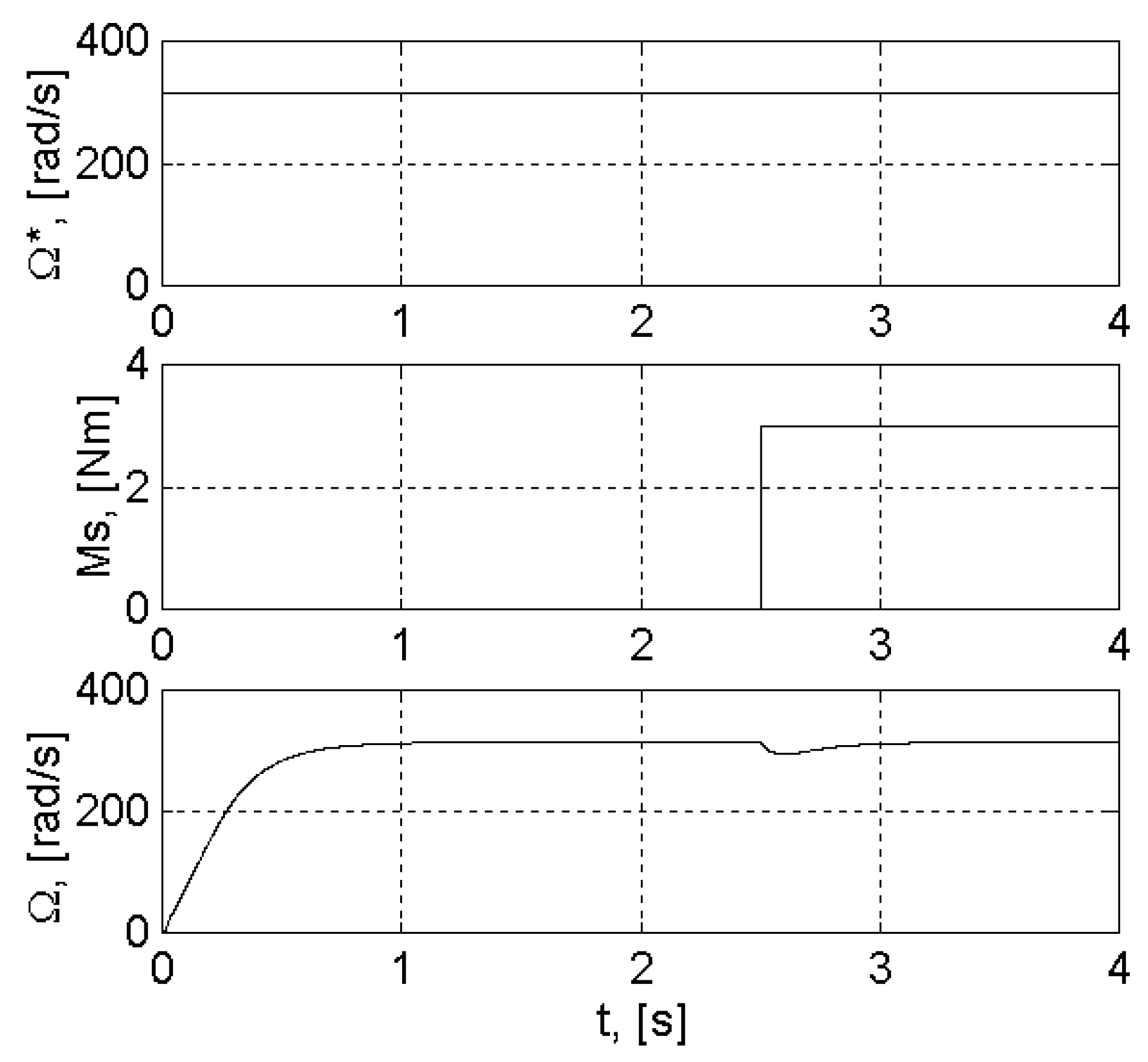
The verification of the input–output stability was performed by transient regime analysis on the model from Figure 1, with the numerical fuzzy controller in Figure 23, having the fuzzy block corrected, in a forced regime, applying step signals at the speed reference input Ω* and at the load torque disturbance input M_s, as in Figure 26.

Figure 26 shows, in case 1 from Table 1, the variations of the input variable Ω* and M_s, which fall into bounded domains, and the way in which the output variable Ω varies. It can be observed, obviously, that the output variable falls within a bounded domain.

The presented characteristics suggest a stable behavior in relation to the control variable Ω* and in relation to the external disturbance M_s.

4. Discussion

The transfer characteristics used in the paper can be obtained by calculations, and they characterize a wide range of fuzzy blocks developed based on the general structure of Mamdani, with various membership functions, rule bases as 3 × 3, 3 × 5, 5 × 5, 5 × 7, and inference methods as prod–sum and min–max, and combinations with defuzzification and the center of gravity. It is recommended to use the defuzzification method with the center of gravity method, which ensures continuous transfer characteristics. Their use allows a grapho-analytical treatment of the stability analysis. These characteristics suggest the existence of the sector property of fuzzy blocks.

The fuzzy PI-type controller can easily be equated with a linear PI controller, for an initial choice of parameters. Equivalence relationships can be used for various types of fuzzy blocks.

The steady state of the fuzzy controller assures a stable equilibrium point.

The vague state portrait of the rule base assures a stable behavior. The rule bases used for the fuzzy controller ensure, in general, the stabilization of the speed regulation system.

The analysis performed on the linear part of the control system shows that it is ε-stable and requires a non-linear part located in a sector [K_min, K_max].

The non-linearity of the control structure, which contains a fuzzy block, falls into a sector of the form [0, K]. There are two causes: one, the use of trapezoidal membership functions, which introduce saturations at the ends of universes of discourse; and two, the use of saturation elements at the inputs of the fuzzy block. It is specified that in order to ensure stability, the characteristic of non-linearity must be corrected, so that it is located in a sector of the form [K_min, K_max].

The correction made on the non-linear part does not change the non-linear character of the fuzzy block, and it can place the non-linearity in a domain that can be conveniently chosen. The values of the two correction coefficients can be chosen according to the type of fuzzy block, so that the characteristic of non-linearity is found in the sector [K_min, K_max], which ensures the absolute global internal stability of the control system. The stability analysis shows that the system can be globally asymptotically internally stable if the recommended correction is applied.

The circle criterion can easily be applied in practice, requiring the frequency characteristics of the linear part, which can be obtained by experimental measurements.

Ensuring internal stability leads to obtaining external stability.

5. Conclusions

The object of the stability analysis performed in the paper was a speed regulation system of an electric drive with a direct current motor, in which a speed regulator of PI fuzzy-type was used. The analysis was undertaken theoretically for the general case, and was applied on a particular case for which the experimental values of the parameters taken into account were given. Any other particular case could be approached with the method presented in the paper. Mamdani’s structure is general, and a multitude of regulator configurations can be considered for such an analysis. The method can be applied to any type of fuzzy controller that has a Mamdani structure, to any type of rule base, for example, 3 × 3, 3 × 5, 5 × 5 or 7 × 7, for min–max and sum–prod inferences, or combinations thereof. The most common fuzzy blocks in practice often have the property of the sector on their universes of discourse, and therefore, the method of analyzing the stability of the motor speed control system presented in the paper can be widely used in practice. The paper demonstrates that the non-linearity of the fuzzy controller can be framed in a sector that ensures the stability of the control system. All the fuzzy controllers mentioned above have transfer characteristics with the sector property. The transfer characteristics provide values, data, and information that can be used in the equivalence of the regulator and in the stability analysis.

The relationships for equivalence of the fuzzy PI controller may be used for any kind of fuzzy block, and may be also used in the equivalence of PD and PID fuzzy controllers.

The characteristic of the regulator can be corrected with the help of two correction coefficients. The values of the two correction coefficients can be chosen depending on the type of fuzzy block, so that the characteristic of non-linearity is found in the sector [K_min, K_max], which ensures the absolute global asymptotic stability of the system.

The paper offers detailed indications for correction characteristics of non-linearity and determination of the stability sector.

The limitations of the method appear when a mathematical model of the linear part cannot be determined, when the frequency characteristics of the linear part cannot be drawn, and when the fuzzy block does not meet the required sector conditions.

The corrections made in the paper on fuzzy blocks can be widely applied to other control systems based on fuzzy PI controllers. This can provide stabilization for wider classes of control systems based on fuzzy logic.

If internal stability is ensured, the external BIBO type stability can be demonstrated.

The presented method uses the frequency characteristics of the linear part, which are easy to obtain in practice by frequency analysis, for various types of electric drive.

The analysis can be developed similarly in the cases of other electric motors widely used in practice, such as induction or permanent magnet synchronous motors.

The most common fuzzy blocks in practice often have sector property over their universes of discourse, and therefore the method of analyzing the stability of the DC motor speed control system presented in the paper can be widely used in practice.

This analysis could be developed similarly in other cases of industrial processes.