Article

Multiple Loop Fuzzy Neural Network Fractional Order Sliding Mode Control of Micro Gyroscope

1
College of Mechanical and Electrical Engineering, Hohai University, Changzhou 213022, China
2
Jiangsu Key Laboratory of Power Transmission and Distribution Equipment Technology, Changzhou 213022, China
*
Author to whom correspondence should be addressed.
Mathematics 2021, 9(17), 2124; https://doi.org/10.3390/math9172124
Submission received: 20 August 2021 / Revised: 27 August 2021 / Accepted: 29 August 2021 / Published: 1 September 2021
(This article belongs to the Special Issue Theory and Applications of Neural Networks)

Abstract

:
In this paper, an adaptive double feedback fuzzy neural fractional order sliding control approach is presented to solve the problem that lumped parameter uncertainties cannot be measured and the parameters are unknown in a micro gyroscope system. Firstly, a fractional order sliding surface is designed, and the fractional order terms can provide additional freedom and improve the control accuracy. Then, the upper bound of lumped nonlinearities is estimated online using a double feedback fuzzy neural network. Accordingly, the gain of switching law is replaced by the estimated value. Meanwhile, the parameters of the double feedback fuzzy network, including base widths, centers, output layer weights, inner gains, and outer gains, can be adjusted in real time in order to improve the stability and identification efficiency. Finally, the simulation results display the performance of the proposed approach in terms of convergence speed and track speed.

1. Introduction

Gyroscope is the basic measurement element in an inertial navigation system, and it can also be used in military [1], aviation, aerospace, bioengineering [2], and other fields. Micro gyroscope with low cost, rapid development, and higher precision represents the development direction of gyroscope technology. In order to satisfy the requirements of different levels of precision in various fields, it is essential to reduce the error and improve the precision of micro gyroscope. In [3], a temperature control system of silicon micro gyroscope based on the fuzzy PID control method and BP neural network is proposed, and it is combined with the temperature compensation method to reduce the error. A MEMS gyroscope based on robust control of the sense mode is developed to improve the reliability of the closed loop system in [4].
For micro gyroscope systems with a certain extent of uncertainty, adaptive control has been widely used. In [5], the neural adaptive control scheme was designed to achieve robust motion control. However, for the condition of parameter uncertainty, adaptive control sometimes cannot achieve effective control performance. The advantages of sliding mode control, which has been combined with adaptive control and widely applied to the control of nonlinear systems, are fast response speed and superb insensitivity to the system uncertainties. An adaptive fuzzy super twisting sliding control scheme is designed to estimate the unknown parameters of micro gyroscope in [6]. In [7], a sliding code control strategy based on adaptive perturbation estimation is proposed for compensating lumped parametric uncertainties of micro tri-axial gyroscopes, and the perturbation observer is employed to estimate the unknown perturbation.
Fuzzy control and neural networks have the ability to approximate unknown smooth functions and have been used in identification and control [8,9,10,11]. The adaptive approximation of the lumped parameter uncertainty of the micro gyroscope model is realized by utilizing various neural networks [12,13], fuzzy system [14,15], and fuzzy neural network approaches [16,17,18,19]. The combination of sliding mode control and a neural algorithm is also used in an active power filter [20,21] and magnetic levitation system [22]. For the purpose of suppressing the chattering phenomenon in sliding mode control, the fractional calculus is introduced into sliding mode control to form a fractional order sliding controller and the chattering is reduced by the genetic attenuation of the fractional order. In the past decade, fractional order sliding mode controllers have been developed for micro gyroscope [23], state of charge estimation of energy lithium-ion batteries [24], antilock braking systems [25], multi-machine power systems [26], and resource systems [27].
Motivated by the above, an adaptive double feedback fuzzy neural network sliding mode control strategy is investigated. This method is applied to solve the problems of uncertain factors in the micro gyroscope system. By combining sliding mode method and adaptive control, the system more effectively can achieve the purpose of system tracking. The novelty and contribution of this work are as follows.
(1)
By adding fractional terms to the sliding surface, the memory characteristics of the fractional calculus operator are used to enhance the continuity of sliding mode control. The switching gain is optimized for the purpose of weakening the system chattering. The designed fractional sliding surface has higher robustness and higher tracking accuracy; meanwhile, the tracking error converges to zero in a finite period of time.
(2)
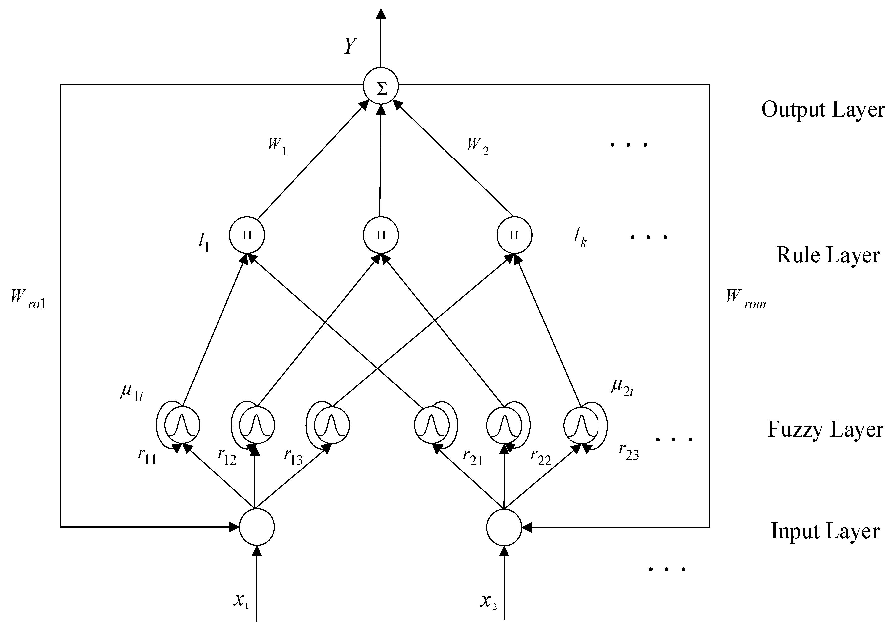
The combination of the fuzzy system and neural network is used to estimate the upper bound of lumped parameter uncertainty, and the true value is replaced by the estimated value as the gain of switching law. Two feedbacks are added to the structure of fuzzy neural control, which has the characteristic of dynamic mapping and can smooth the output of the neural network.
The remainder of the paper is organized as follows. Section 2 presents the dynamic analysis of the micro gyroscope system. Section 3 presents the design of the adaptive fractional order sliding mode controller. Section 4 introduces a double feedback fuzzy neural network fractional order sliding mode control. Section 5 presents the simulation of the proposed method. Finally, Section 6 provides a summary of the full text.

2. Dynamic Analysis of Micro Gyroscope

The micro gyroscope has two working modes: drive mode and sense mode. The measurement accuracy is mainly affected by the stability of the drive mode control. The sense mode is closely related to the measurement result. The simplified micro gyroscope dynamic model is shown in Figure 1.
The rotational coordinate system of the simplified micro gyroscope dynamic model is established and, considering the effect of structural error, the basic dynamic equation can be expressed as follows:
m x ¨ + d x x x ˙ + d x y y ˙ + k x x x + k x y y = u x + 2 m Ω z y ˙
m y ¨ + d x y x ˙ + d y y y ˙ + k x y x + k y y y = u y 2 m Ω z x ˙
where m is the mass of the mass block, Ω z is the angular velocity of the z-axis, d x y is the coupling damping coefficient, d x x and d y y are the damping coefficients, k x y is the coupling stiffness coefficient, k x x is the x-axis stiffness coefficient, k y y is the y-axis stiffness coefficient, and u x and u y are the control inputs.
The dynamic model is transformed into dimensionless form to reduce the complexity of the controller design. Dividing both sides of Equations (1) and (2) by the mass block m , the natural resonance frequency ω 0 and the reference length q 0 are used to obtain the dimensionless dynamic model as follows:
q ¨ q 0 + D d m ω 0 q ˙ q 0 + K m ω 0 2 q q 0 = u m ω 0 2 q 0 2 Ω ω 0 q ˙ q 0
where q = x y , q ˙ = x ˙ y ˙ , q ¨ = x ¨ y ¨ , D d = d x x d x y d x y d y y , K = ω x x ω x y ω x y ω y y , u = u x u y , Ω = 0 Ω z Ω z 0 .
Equation (3) can be rephrased as follows:
q ¨ + D q ˙ + K q = u 2 Ω q ˙

3. Fractional-Order Sliding Mode Controller

In view of the lumped system nonlinearities, the micro gyroscope dynamic model can be rephrased as follows:
q ¨ +   K + Δ K q + ( D d + 2 Ω + Δ D ) q ˙ = u + d
where d represents the external disturbances, Δ K represents the uncertainties of unknown parameters K , and Δ D represents the uncertainties of unknown parameters D d + 2 Ω .
The system model in Equation (5) can be rephrased as follows:
q ¨ + K q +   D d + 2 Ω q ˙ = u + f d
where f d is lumped parameter uncertainty, namely, the unknown external disturbances and parameter uncertainties, defined as follows:
f d = d Δ D q ˙ Δ K q
It is assumed that the lumped parameter uncertainty f d has an upper bound that satisfies the following condition:
f d   ρ   ,
where ρ is an unknown positive constant.
We design a fractional-order sliding surface to carry out the tracking of the system because of its looser degree of freedom.
The Caputo fractional derivative of order α of a continuous function f x used in this paper is expressed in the following form:
a D t α f t   =   1 Γ n α a t f n τ t τ α n + 1 d τ , n 1 < α < n d n d t n f t , α = n
where t is the upper bound of the operator, a is the lower bound of the operator, and Γ ( ) represents the Gamma function. For ease of notation, the fractional derivative of order α with the lower bound at 0 can be described as D α instead of 0 D t α .
The fractional order sliding surface is defined as follows:
s = e ˙ + c e + λ D α 1 e
where c and λ are the designed parameter matrices and they are the known position constant; α 1 is the order of the fractional order, and 0 < α < 1 ; e is defined as the tracking error, and e = q q r , where q r represents the actual position; and the expression of e ˙ is e ˙ = q ˙ q ˙ r .
By derivatizing (9), we can obtain the following:
s ˙ = e ¨ + c e ˙ + λ D α e
Substituting the system model in Equation (6) into Equation (10) leads to the following:
s ˙ = c e ˙ + λ D α e + u q ¨ r   D d + 2 Ω q ˙ K q + f d
According to the hitting condition, the following equation can be obtained:
c e ˙ + λ D α e + u q ¨ r   D d + 2 Ω q ˙ K q + f d = 0
The equivalent control law of sliding mode control can be obtained:
u e q = c e ˙ λ D α e + q ¨ r +   D d + 2 Ω q ˙ + K q
The switching law is designed as follows:
u s w = ρ s s
Therefore, the fractional order sliding controller is received as follows:
u = c e ˙ λ D α e + q ¨ r +   D d + 2 Ω q ˙ + K q ρ s s

4. Adaptive Double Feedback Fuzzy Neural Network Fractional-Order Sliding Mode Controller

4.1. Double Feedback Fuzzy Neural Network

In the practical micro gyroscope system, the upper bound of system lumped parameter uncertainties cannot be measured. This is because the system parameters are not constant in different environments and the offline identification method is not applicable. Therefore, the combination of the neural network and fuzzy system is used to estimate the upper bound of the lumped parameter uncertainties in real time, in order to replace its truth value as the switching gain. Compared with the large amount of data and workspace required for offline identification, the fuzzy neural network can make use of the experience of experts to induce learning, improve the efficiency of online identification, and have the capabilities of self-learning and self-organization.
In the fuzzy system, the design of membership functions, fuzzy rules, and fuzzy sets is based on knowledge from experience. The self-learning ability of the neural network is introduced into the fuzzy system, so that the membership functions and fuzzy rules can be modified and improved in the continuous learning of the fuzzy system. In addition, the inference ability of the fuzzy system is greatly improved. The system has dynamic characteristics in practical work, so the dynamic fuzzy neural network (DFNN) is more suitable for the micro gyroscope system. The double feedback fuzzy neural network is established in the fuzzy neural network by adding a recurrent unit, fuzzy rules are gradually formed in the learning process, and the free parameters of the membership function are tuned. Thus, the network structure can be optimized and the prediction accuracy and generalization ability can be enhanced.
The four-layer fuzzy neural network with two-layer closed-loop dynamic feedback mainly includes an input layer, fuzzy layer, rule layer, and output layer, and the neural network structure is shown in Figure 2. The output is the estimation value of the upper bound ρ ^ of lumped parameter uncertainties. In its external feedback loop and internal feedback loop, the output signal of the previous step will be stored and fed back to the layer via the feedback channel, and the calculation will be performed again. Because the double feedback fuzzy neural network has two feedback loops, it can store more information, so it has a better effect on the unknown nonlinear model approximation. The parameters can be adjusted adaptively according to adaptive laws to achieve the optimal values.
Each layer of the double feedback fuzzy neural network is described as follows.
Layer I: Input Layer
It is composed of a signal receiving node to complete the transmission of input signal X = x 1 , x 2 , , x m T R m × 1 , and the neurons of this layer can receive the output signal e x Y , which is fed back by the output layer neurons. The output of each node is described as follows:
θ m = x m W r o m e x Y
The output layer and the input layer are connected by the weight W r o = W r o 1 ,   W r o 2 ,   ,   W r o m T R m × 1 of the outer layer feedback fuzzy neural network. The output is θ = θ 1 ,   θ 2 ,   ,   θ m T R m × 1 and the feedback signal of this layer is defined as e x Y .
Layer II: Fuzzy Layer
Gaussian function is used as the membership function to complete the calculation of membership function and adjust the number of neurons according to the situation. The center is defined as c = c 11 ,   c 12 ,   ,   c 1 i ,   c 21 ,   c 22 ,   ,   c 2 i ,   ,   c m 1 ,   c m 2 ,   ,   c m i T R m i × 1 and the base width is defined as b = b 11 ,   b 12 ,   ,   b 1 i ,   b 21 ,   b 22 ,   ,   b 2 i ,   ,   b m 1 ,   b m 2 ,   ,   b m i T R m i × 1 . There are feedback connection weights of the inner regression fuzzy neural network in this layer. The inner regression fuzzy neuron will feed the calculation results of the previous membership function back to its input end, and as a part of this input, the Gaussian function is calculated together, thereby completing the feedback of the signal, and setting the output of the layer as follows:
μ m i = exp θ m + r m i e x μ m i c m i 2 b m i 2
The feedback signal of this layer is defined as e x μ m i .
Layer III: Rule Layer
The output of each node is the product of all input signals of the node, that is,
l k = μ 1 i μ 2 i μ m i
where the output is l = l 1 ,   l 2 ,   ,   l k T R k × 1 .
Layer IV: Output Layer
Neurons in this layer are connected to neurons in the rule layer by weight W = W 1 ,   W 2 ,   ,   W k T R k × 1 . After the calculation of the output Y , the output signal is fed back to the input layer neurons.
Y = W T l = W 1 l 1 + W 2 l 2 + + W k l k

4.2. Design and Stability of the Adaptive Double Feedback Fuzzy Neural Network Fractional-Order Sliding Mode Controller
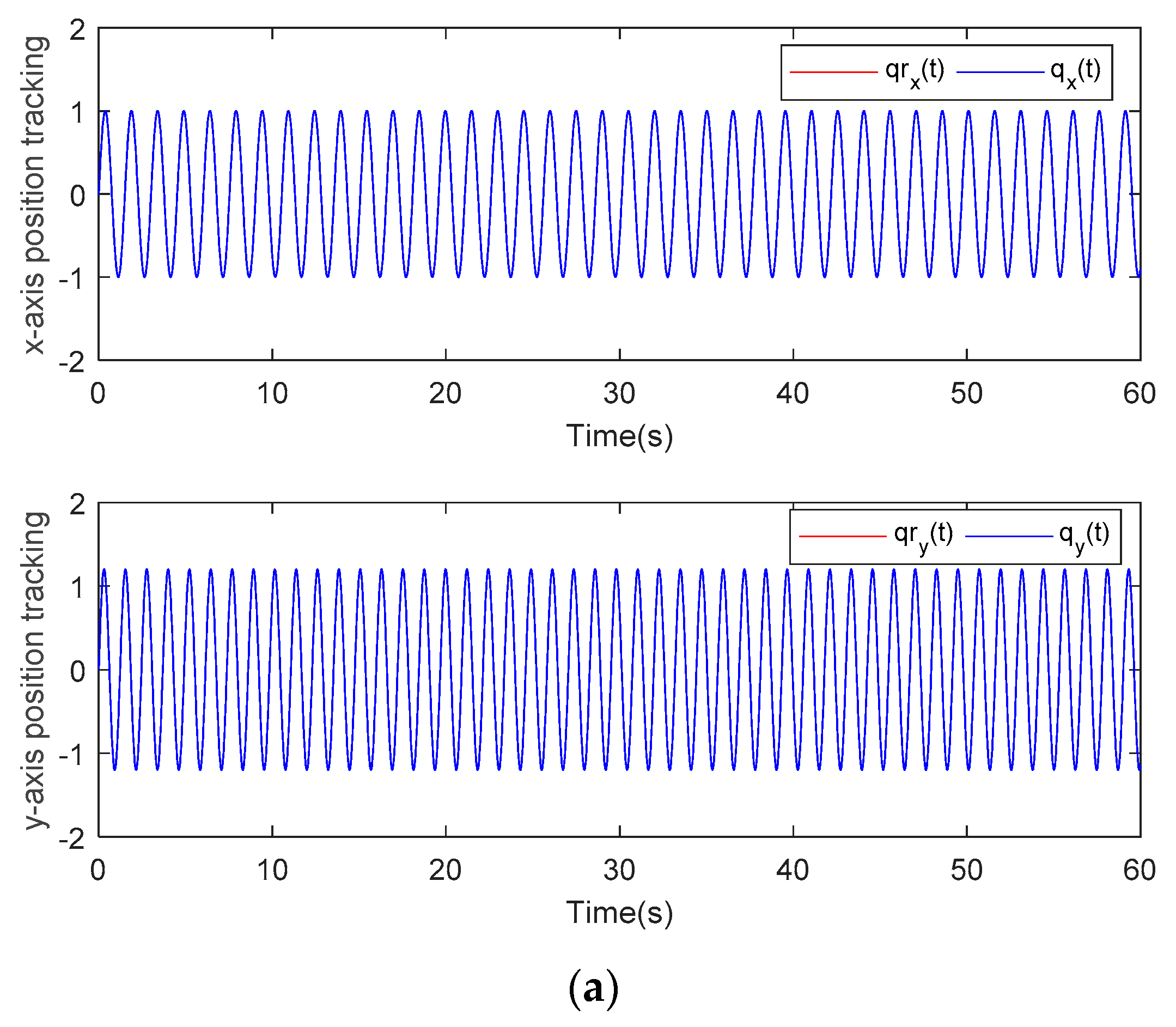
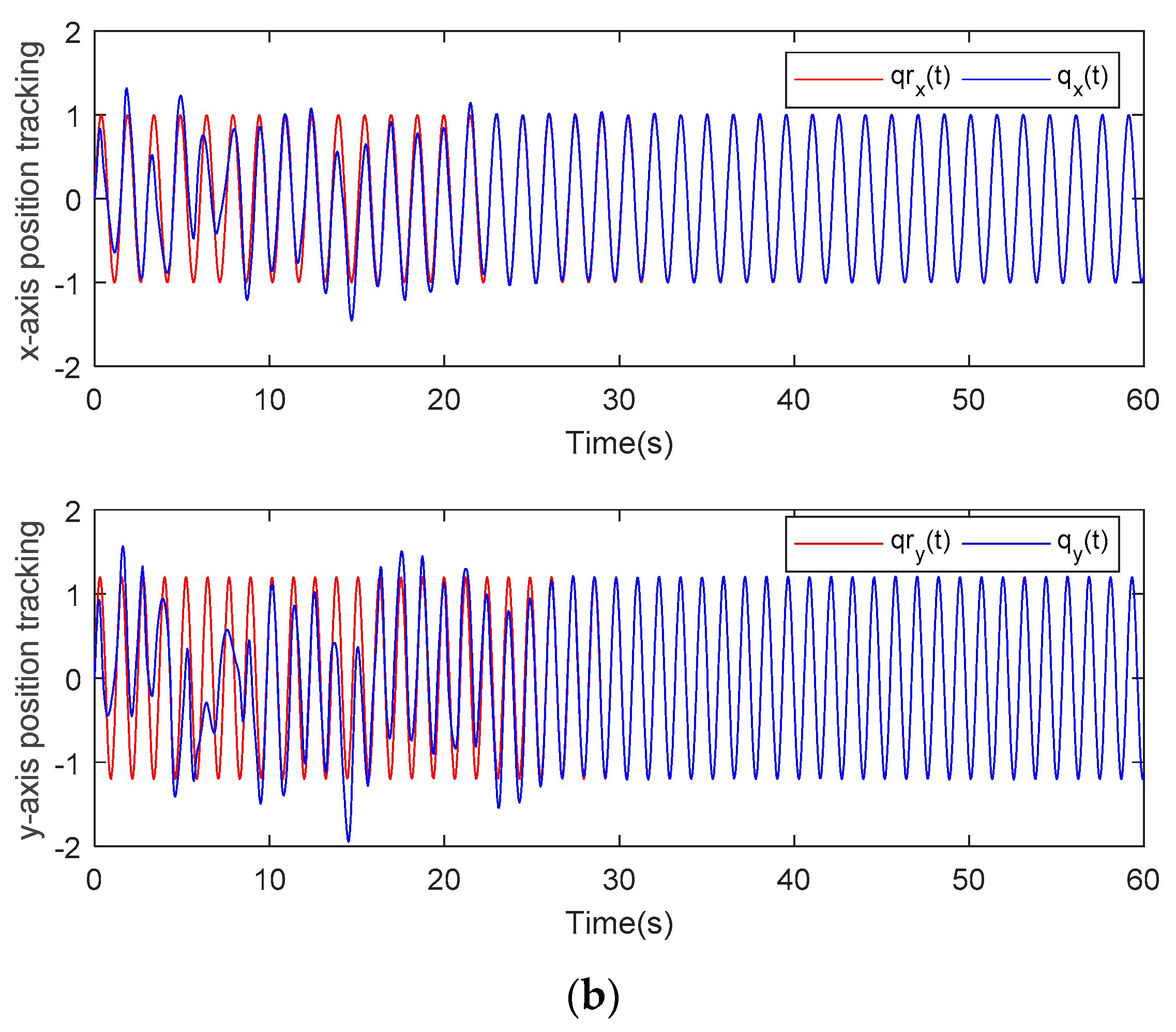
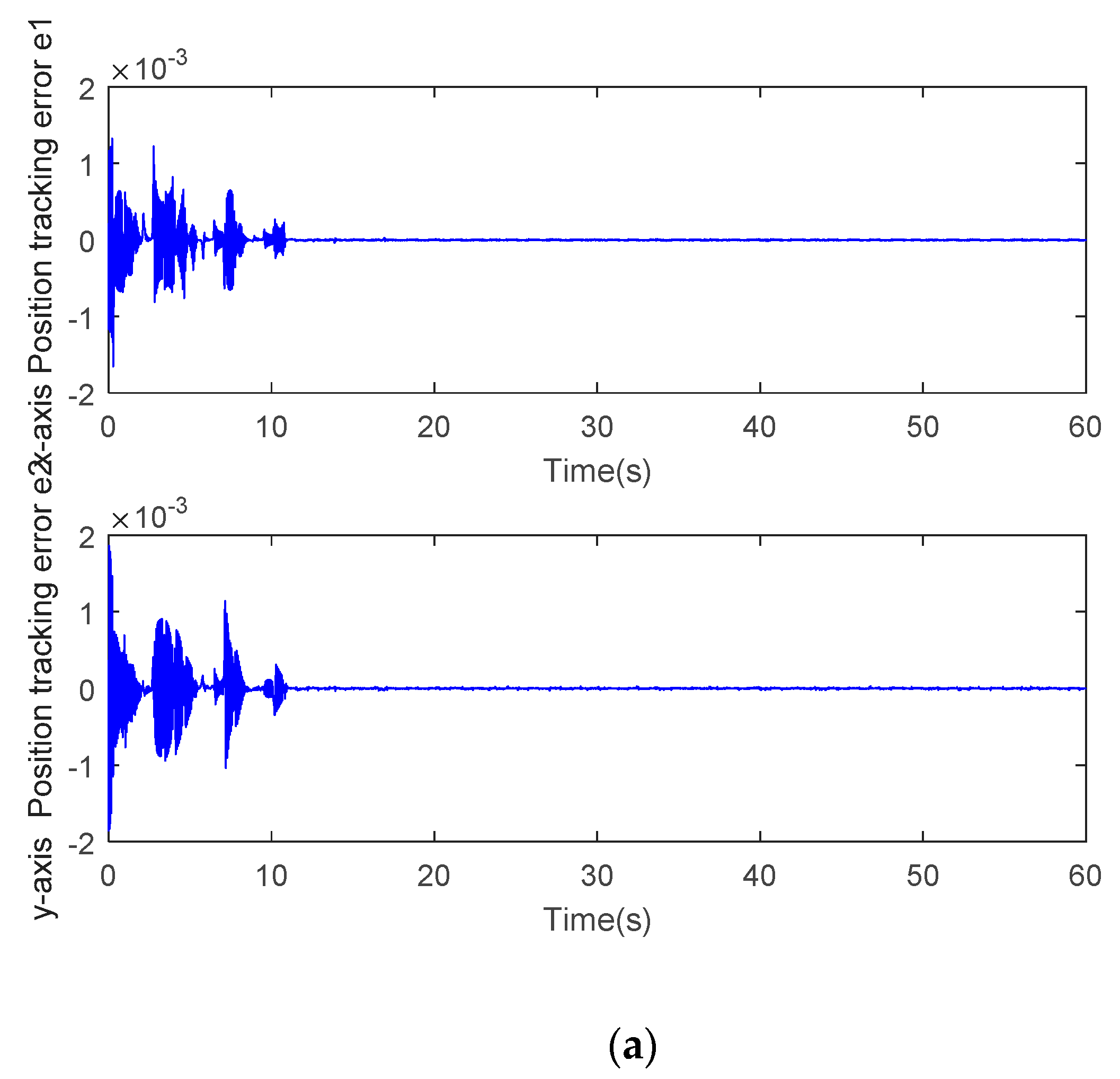
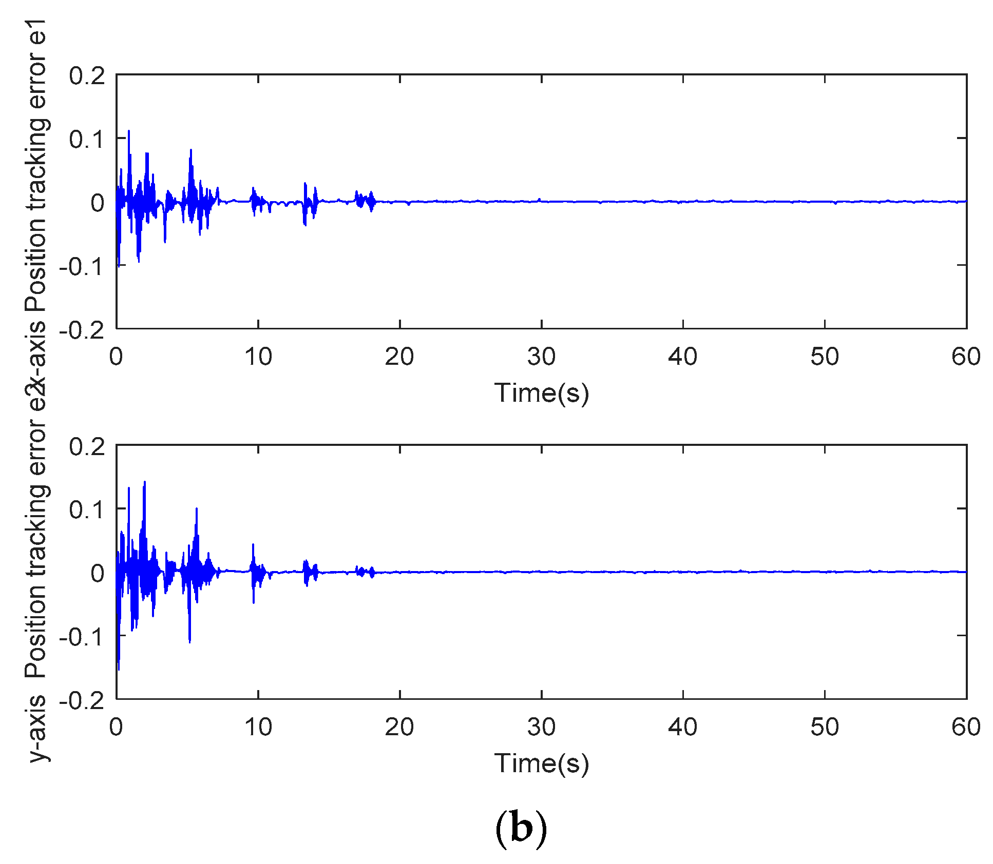
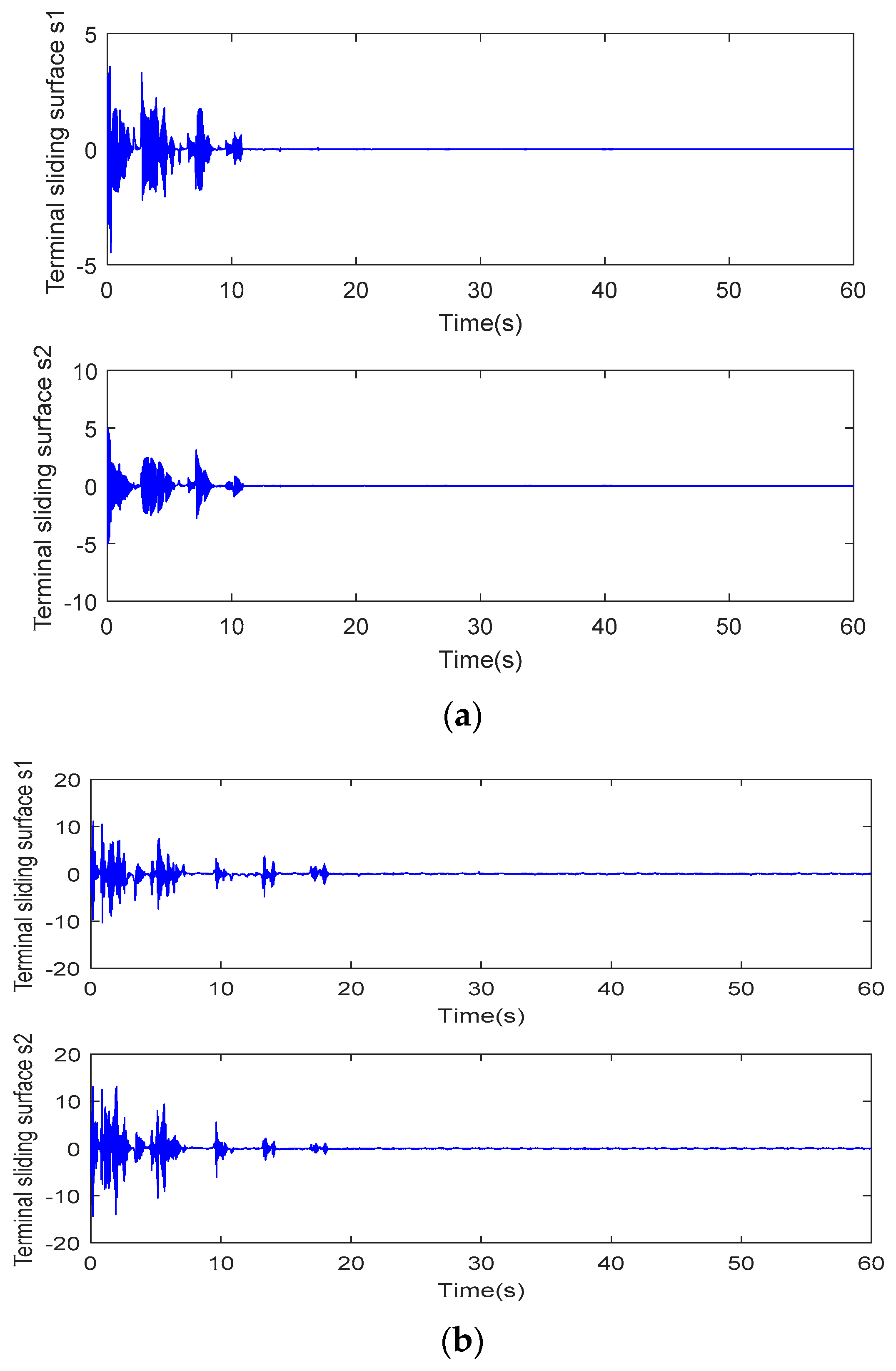
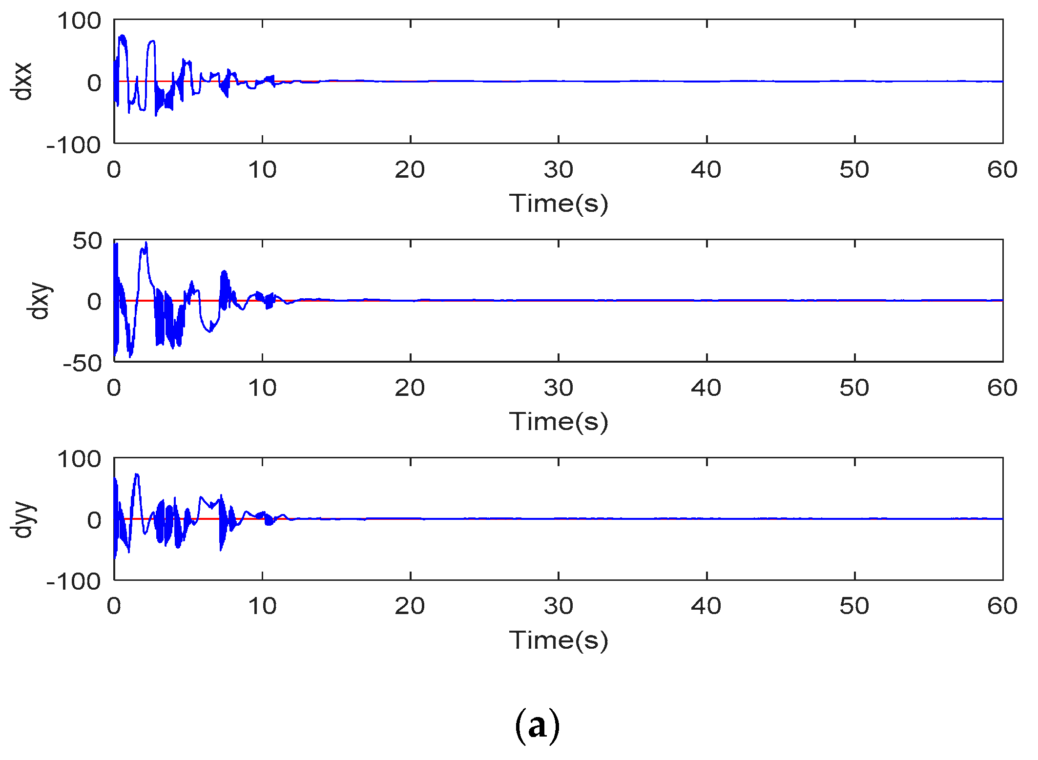
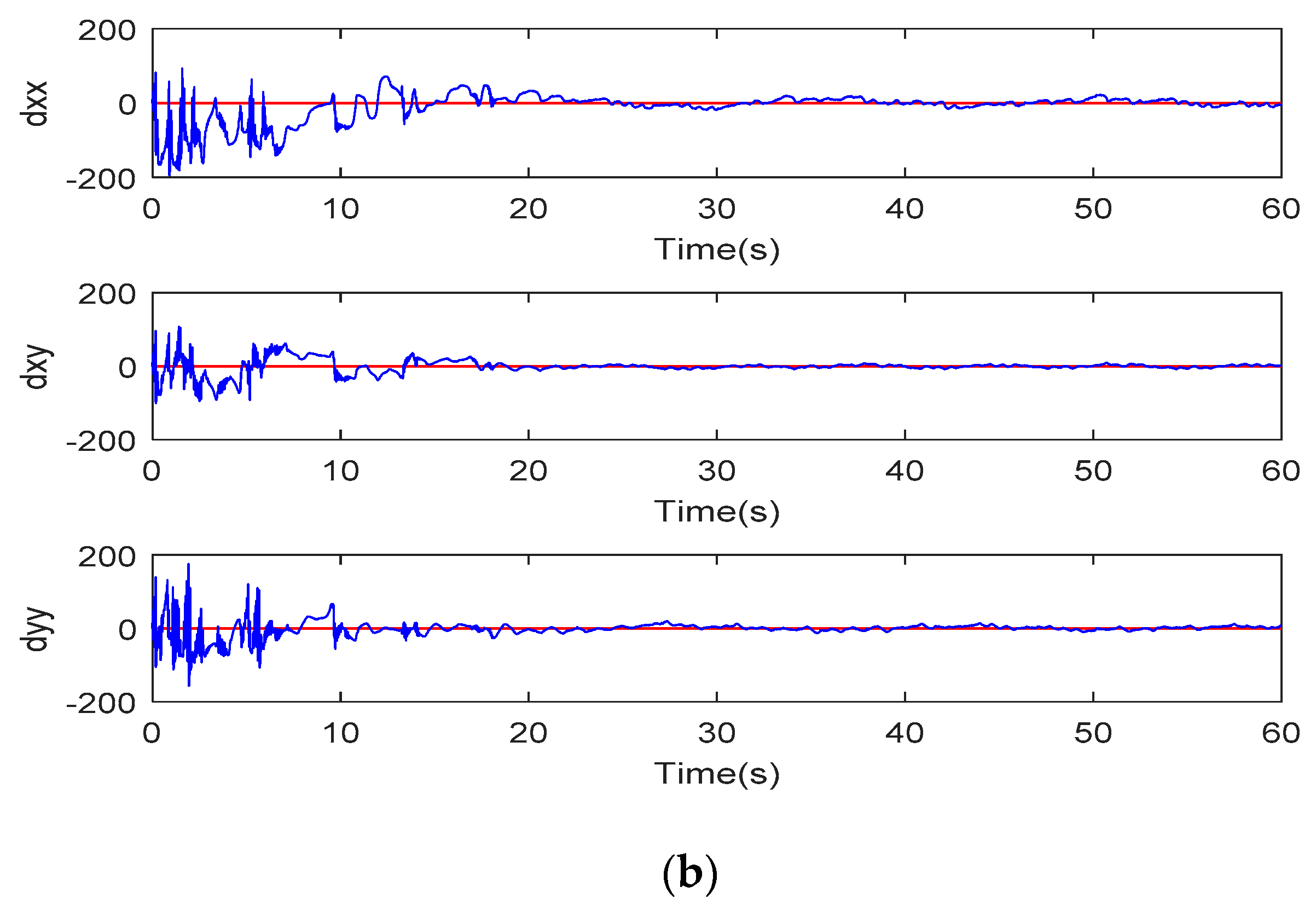
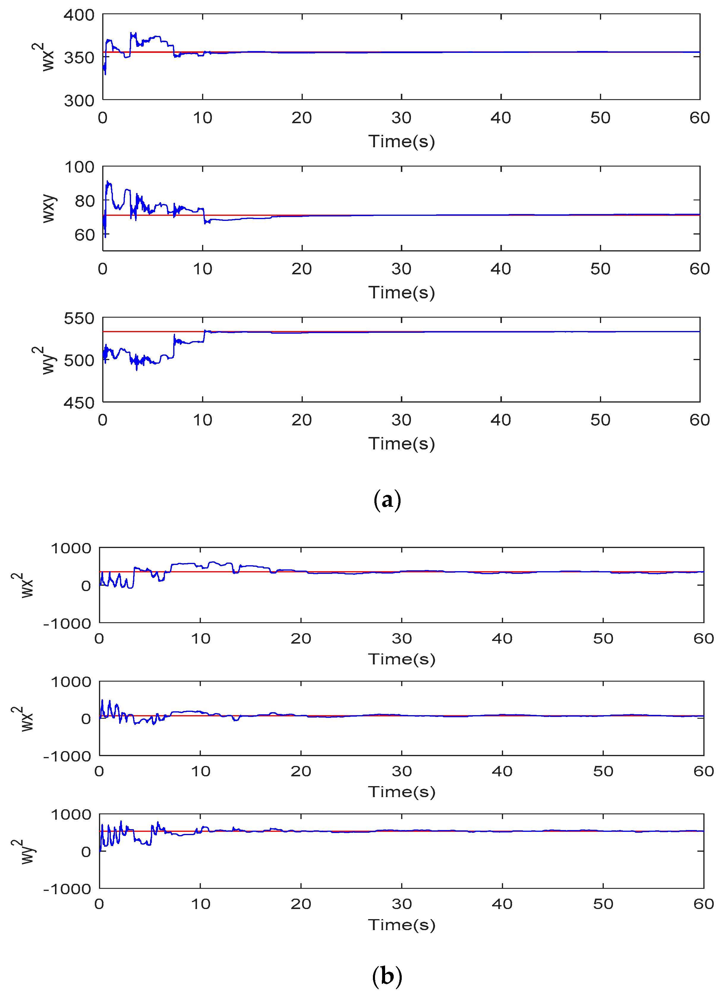
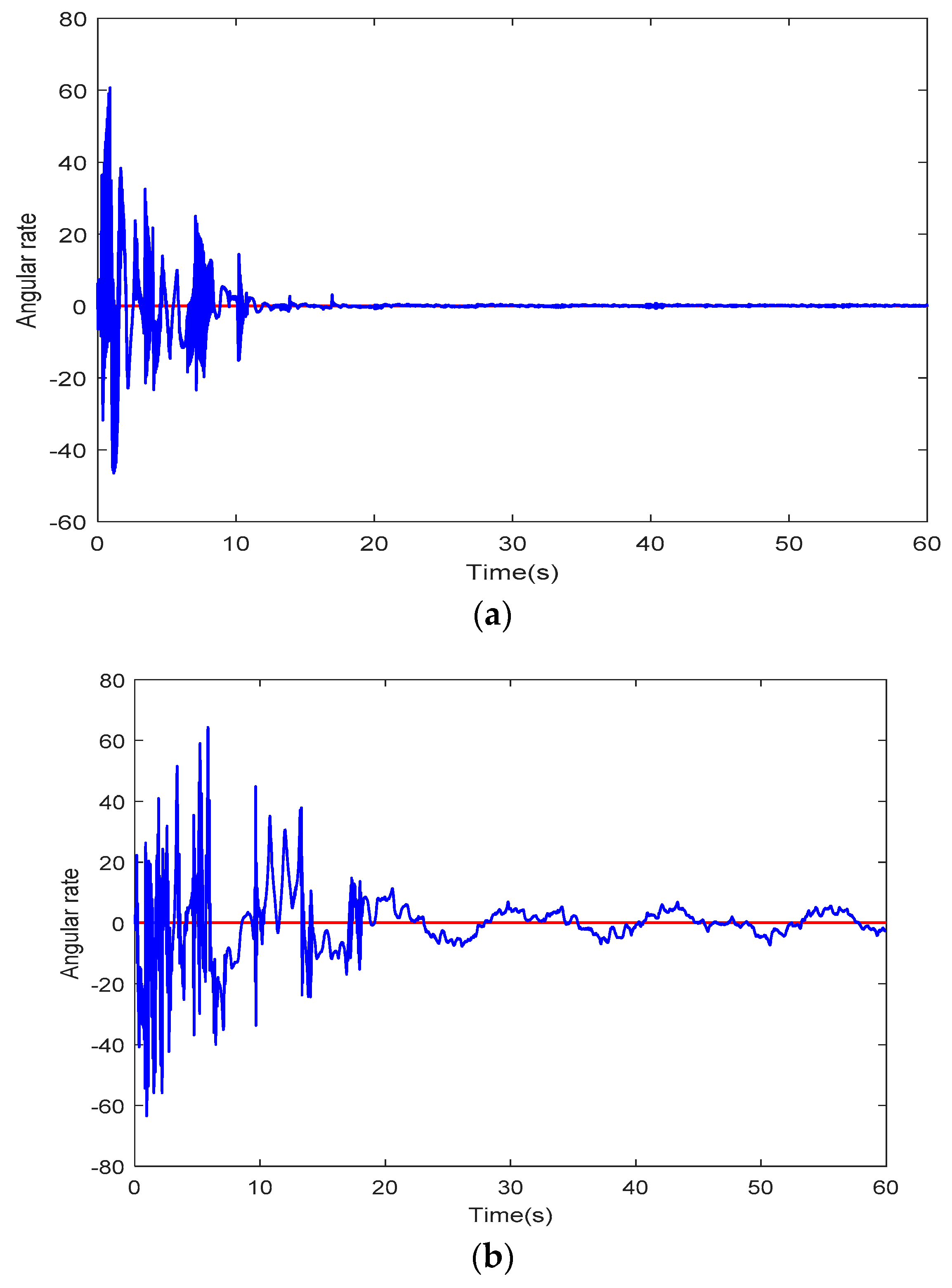
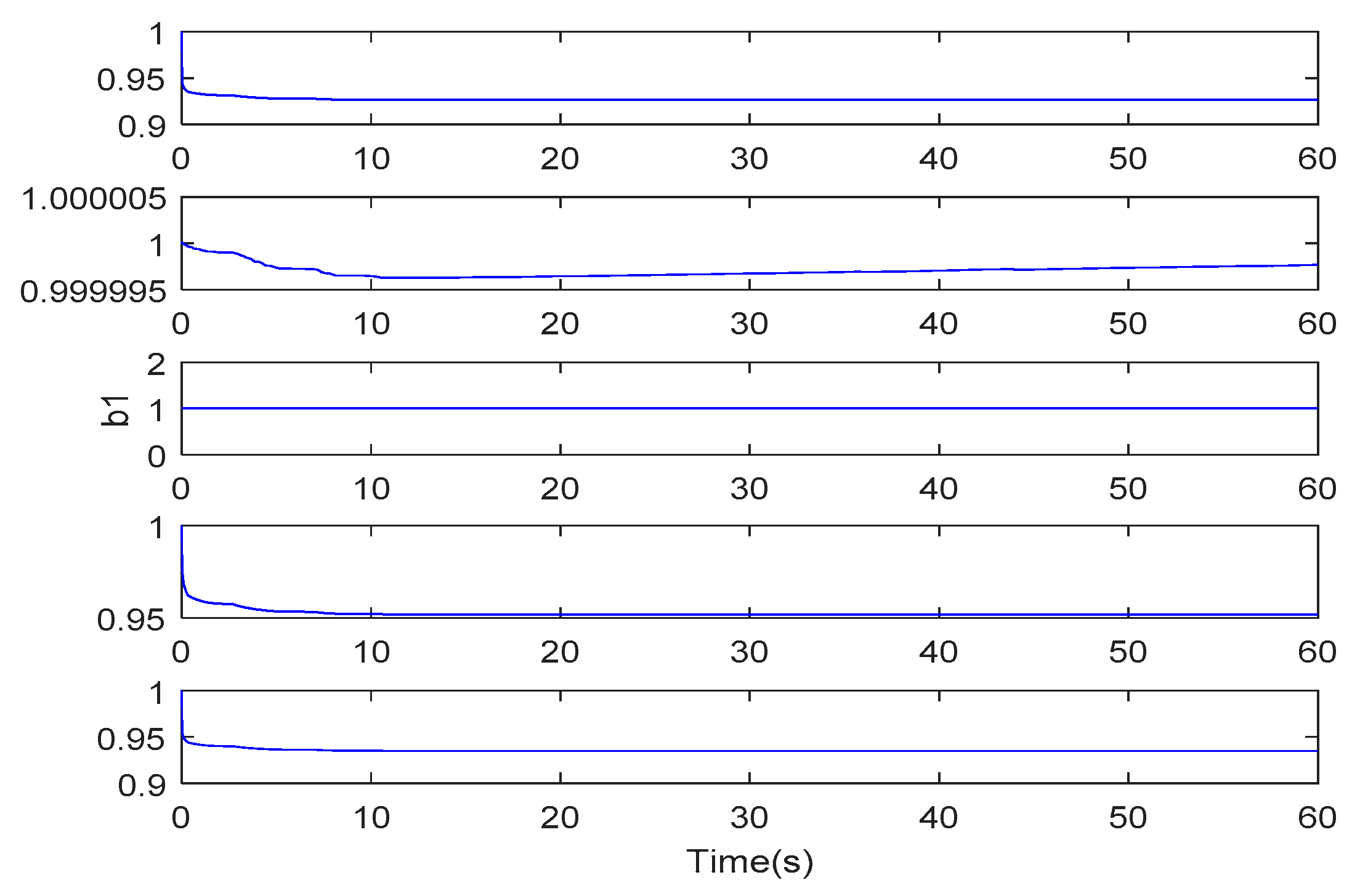
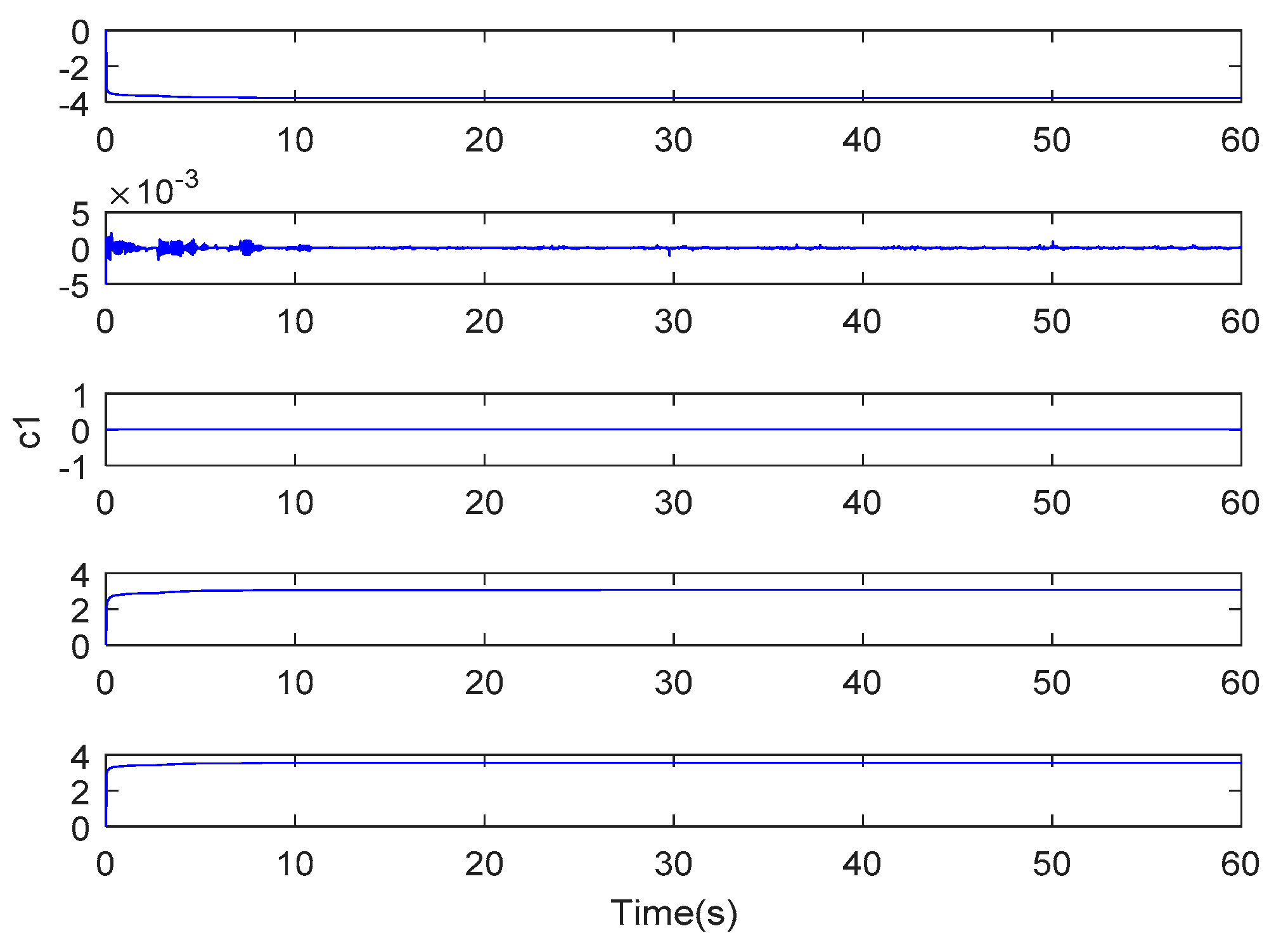
The developed control law in (15) cannot be realized because of the unknown upper bound of lumped parameter uncertainties. DFNN is adopted in this part to approximate the unknown upper bound of the lumped uncertainty online. Figure 3 is a block diagram of the adaptive double feedback fuzzy neural fractional sliding mode control system, where the proposed controller is designed in the form of (15). Considering the strong ability of estimating any smooth functions using the FNN, a DFNN approximator could be considered to deal with the unknown part and used to estimate the upper bound of the lumped uncertainty of lumped parameter uncertainties, which is used as the gain of switching control law. An adaptive controller is utilized to update all unknown parameters of the micro gyroscope system.
The upper bound of lumped parameter uncertainties is approximated using double feedback fuzzy neural networks, namely,
ρ ^ = W ^ T l ^
where W ^ is the estimated value of fuzzy neural network weight; l ^ is the function of x ,   c ^ ,   b ^ ,   r ^ ,   W ^ r o ; the input of double feedback fuzzy neural network is x = q q ˙ T R 2 × 1 ; and q and q ˙ are the measurable signals.
The following reasonable assumptions are made for the established double feedback fuzzy neural network to prove the stability of the proposed system:
Assumption 1.
There are optimal weights  W  of neural network, optimal center  c  of Gaussian function, optimal base width  b  of Gaussian function, optimal inner feedback weights  r , and optimal outer feedback weights  W r o , which make the following inequalities valid:
ε   =   W T l ρ   < ε
where  ε  is the mapping error, the upper bound of the error is defined as  ε , and both  ε  and  ε   are small positive constants.
Assumption 2.
ρ , f d , and ε satisfy the following relationship:
ρ   f d   > ε
Therefore, the control law u of Equation (15) can be adjusted as follows:
u = c e ˙ λ D α e + q ¨ r +   D d + 2 Ω q ˙ + K q ρ ^ s s
Using the Lyapunov stability theory, the unknown real values are replaced by the estimates of parameter matrices, weights, and center. The estimates of parameter matrix D ^ d ,   K ^ , and Ω ^ ; the estimates of neural network weight W ^ ; the estimates of center c ^ ; the estimates of base width b ^ ; the estimates of inner feedback weight r ^ ; and the estimates of outer feedback weight W ^ r o are designed. Online real-time updating can thus be realized.
The parameters’ estimated errors are defined as follows:
D ˜ d = D d D ^ d Ω ˜ = Ω Ω ^ K ˜ = K K ^ W ˜ = W W ^ c ˜ = c c ^ b ˜ = b b ^ r ˜ = r r ^ W ˜ r o = W r o W ^ r o l ˜ = l l ^
Substituting (24) into (23), the estimated control law is obtained:
u = c e ˙ λ D α e + q ¨ r +   D ^ d + 2 Ω ^ q ˙ + K ^ q ρ ^ s s
That is, the adaptive double feedback fuzzy neural fractional-order sliding controller.
Because D d , Ω , K , W , l , b , c , r , and W r o are constant values,
D ˜ ˙ d = D ^ ˙ d Ω ˜ ˙ = Ω ^ ˙ K ˜ ˙ = K ^ ˙ W ˜ ˙ = W ^ ˙ c ˜ ˙ = c ^ ˙ b ˜ ˙ = b ^ ˙ r ˜ ˙ = r ^ ˙ W ˜ ˙ r o = W ^ ˙ r o l ˜ ˙ = l ^ ˙
Substituting Equations (24) and (25) into micro gyroscope expression (6) generates the following:
c e ˙ + λ D α e + q ¨ q ¨ r =   D ^ d + 2 Ω ^ q ˙   D d + 2 Ω q ˙ K q + K ^ q Δ K q Δ D d q ˙ ρ ^ s s + d
Using Equation (11) yields the following:
s ˙ =   D ^ d + 2 Ω ^ q ˙   D d + 2 Ω q ˙ K q + K ^ q Δ K q Δ D d q ˙ ρ ^ s s + d
Substituting the lumped parameter uncertainties of the system, and simplifying Equation (28), we obtain the following:
s ˙ = D ˜ d + 2 Ω ˜ q ˙ + K ˜ q + f ρ ^ s s
The Lyapunov function is selected as follows:
V = 1 2 s T s + 1 2 t r D ˜ d M 1 D ˜ d T   +   1 2 t r K ˜ N 1 K ˜ T   +   1 2 t r Ω ˜ P 1 Ω ˜ T + 1 2 η 1 W ˜ T W ˜ + 1 2 η 2 c ˜ T c ˜ + 1 2 η 3 b ˜ T b ˜ + 1 2 η 4 r ˜ T r ˜ + 1 2 η 5 W ˜ r o T W ˜ r o
where M = M T > 0 , P = P T > 0 , N = N T > 0 ; η 1 , η 2 , η 3 , η 4 , and η 5 are positive constants and represent the learning rate of the fuzzy neural network. Let
ξ = 1 2 t r D ˜ d M 1 D ˜ d T   +   1 2 t r K ˜ N 1 K ˜ T   +   1 2 t r Ω ˜ P 1 Ω ˜ T + 1 2 η 1 W ˜ T W ˜ + 1 2 η 2 c ˜ T c ˜ + 1 2 η 3 b ˜ T b ˜ + 1 2 η 4 r ˜ T r ˜ + 1 2 η 5 W ˜ r o T W ˜ r o
Differentiating (30) with respect to time, combining the contents of Assumption 3 and substituting Equation (31) yields the following:
V ˙ = s T D ˜ d + 2 Ω ˜ q ˙ + K ˜ q + f ρ ^ s s   +   ξ ˙ = s T D ˜ d + 2 Ω ˜ q ˙ + K ˜ q + f W ^ T l ^ s s   +   ξ ˙ s T D ˜ d + 2 Ω ˜ q ˙ + K ˜ q + f     s W ^ T l ^ ρ + ρ   +   ξ ˙ = s T D ˜ d + 2 Ω ˜ q ˙ + K ˜ q + f ρ   +   s ρ W ^ T l ^   +   ξ ˙ = s T D ˜ d + 2 Ω ˜ q ˙ + K ˜ q + f ρ   +   s W T l W ^ T l ^ + ε   +   ξ ˙ = s T D ˜ d + 2 Ω ˜ q ˙ + K ˜ q + f ρ   +   s W ^ T l ˜ + W ˜ T l ˜ + W ˜ T l ^ + ε   +   ξ ˙
The approximation error is defined as W ˜ T l ˜ + ε = ε 0 , and Equation (31) can be simplified as follows:
V ˙ s T D ˜ d + 2 Ω ˜ q ˙ + K ˜ q + f ρ   +   s W ^ T l ˜ + W ˜ T l ^ + ε 0   +   ξ ˙
l ˜ is expressed in the Taylor series as follows:
l ˜ = l c c = c c c ^   +   l b b = b b b ^   +   l r r = r r r ^ + l W r o W r o = W r o W r o W ^ r o   +   Δ = l c c ˜ + l b b ˜ + l r r ˜ + l W r o W ˜ r o + Δ
where Δ is a high-order term, l R 5 × 1 , and the coefficient matrices are expressed as follows:
l c = l 1 c T l 2 c T l k c T = l 1 c 1 l 1 c 2 l 1 c i l 2 c 1 l 2 c 2 l 2 c i l k c 1 l k c 2 l k c i k × m i ,
l b = l 1 b T l 2 b T l k b T = l 1 b 1 l 1 b 2 l 1 b i l 2 b 1 l 2 b 2 l 2 b i l k b 1 l k b 2 l k b i k × m i ,
l r = l 1 r T l 2 r T l k r T = l 1 r 1 l 1 r 2 l 1 r i l 2 r 1 l 2 r 2 l 2 r i l k r 1 l k r 2 l k r i k × m i ,
l W r o = l 1 W r o T l 2 W r o T l k W r o T = l 1 W r o 1 l 1 W r o 2 l 1 W r o i l 2 W r o 1 l 2 W r o 2 l 2 W r o i l k W r o 1 l k W r o 2 l k W r o i k × m i .
Substituting Equation (33) into Equation (32) leads to the following:
V ˙ s T D ˜ d + 2 Ω ˜ q ˙ + K ˜ q + f ρ   +   s W ^ T l c c ˜ + l b b ˜ +   l r r ˜ + l W r o W ˜ r o + Δ   +   W ˜ T l ^ + ε 0   +   t r D ˜ d M 1 D ˜ ˙ d T +   t r Ω ˜ P 1 Ω ˜ ˙ T   +   t r K ˜ N 1 K ˜ ˙ T   +   1 η 1 W ˜ ˙ T W ˜   +   1 η 2 c ˜ ˙ T c ˜ +   1 η 3 b ˜ ˙ T b ˜ + 1 η 4 r ˜ ˙ T r ˜ + 1 η 5 W ˜ ˙ r o T W ˜ r o .
Because D d , K , and Ω are symmetric matrices, and for matrix D d , there is a scalar s T D ˜ d q ˙ = q ˙ T D ˜ d s , the following can be obtained:
s T D ˜ d q ˙ = 1 2 s T D ˜ d q ˙ + q ˙ T D ˜ d s
Similarly, the equations for matrices K and Ω can be obtained:
s T K ˜ q ˙ = 1 2 s T K ˜ q + q T K ˜ s
s T Ω ˜ q ˙ = 1 2 s T Ω ˜ q ˙ q ˙ T Ω ˜ s
Substituting (35)–(37) into (34) gives the following:
V ˙ s T f ρ   +   s W ^ T l c c ˜ + l b b ˜ + l r r ˜ + l W r o W ˜ r o + Δ +   W ˜ T l ^ + ε 0   +   1 η 1 W ˜ ˙ T W ˜   +   1 η 2 c ˜ ˙ T c ˜ + 1 η 3 b ˜ ˙ T b ˜ + 1 η 4 r ˜ ˙ T r ˜ +   1 η 5 W ˜ ˙ r o T W ˜ r o + t r D ˜ d M 1 D ^ ˙ d T +   1 2 s T q ˙ + q ˙ T s +   t r K ˜ N 1 K ^ ˙ T + 1 2 s T q + q T s +   t r Ω ˜ P 1 Ω ^ ˙ T + 1 2 2 q ˙ s T 2 s q ˙ T
To ensure that V ˙ 0 , let t r D ˜ d M 1 D ^ ˙ d T + 1 2 s T q ˙ + q ˙ T s   = 0 , s W ˜ T l ^ + 1 η 1 W ˜ T W ˜ ˙ = 0 , t r K ˜ N 1 K ^ ˙ T + 1 2 s T q + q T s   = 0 , s W ^ T l c c ˜ + 1 η 2 c ˜ ˙ T c ˜ = 0 , t r Ω ˜ P 1 Ω ^ ˙ T + 1 2 2 q ˙ s T 2 s q ˙ T   = 0 , s W ^ T l b b ˜ + 1 η 3 b ˜ ˙ T b ˜ = 0 , s W ^ T l r r ˜ + 1 η 4 r ˜ ˙ T r ˜ = 0 , s W ^ T l W r o W ˜ r o + 1 η 5 W ˜ ˙ r o T W ˜ r o = 0 , the adaptive laws of D ^ ,   K ^ ,   Ω ^ ,   W ^ ,   c ^ ,   b ^ ,   r ^ and W ^ r o are calculated as follows:
D ^ ˙ d T = 1 2 M q ˙ s T + s q ˙ T K ^ ˙ T = 1 2 N q s T + s q T Ω ^ ˙ T = P q ˙ s T s q ˙ T W ^ ˙ T =   η 1 s l ^ c ^ ˙ T = η 2 s W ^ T l c b ^ ˙ T = η 3 s W ^ T l b r ^ ˙ T = η 4 s W ^ T l r W ^ ˙ r o T = η 5 s W ^ T l W r o
Substituting the adaptive laws in Equation (39) into Equation (38), and according to Assumption 2, we can obtain the following:
V ˙ s T f ρ   +   s W ^ T Δ + ε 0     s f     ρ   +   s W ^ T Δ + ε 0   s ε ε 0 W ^ T Δ
Assume that W ^ T Δ has upper bound Δ d , and Δ d , ε , and ε 0 satisfy ε > ε 0 + Δ d , that is, V ˙ 0 is guaranteed and V is semi-negative, namely, the tracking trajectory can reach the designed fractional-order sliding surface and stay on it. For the integral of inequality V ˙ s ε ε 0 W ^ T Δ , 0 t s d t 1 ε     ε 0     Δ d V t     V 0 can be obtained, because V 0 and V t are bounded, and V t is non-increasing, so 0 t s ε     ε 0     Δ d d t is bounded. According to Barbalat lemma, lim t s t   = 0 can be obtained, then it can be shown that the system is asymptotically stable.

5. Simulation Study

The proposed adaptive double feedback fuzzy neural network fractional-order sliding mode control method is simulated with MATLAB/Simulink. The selection of the dimensional parameters of gyroscope is shown in Table 1.
In order to make it easier to implement the controller design, it is essential to perform dimensionless processing on the system mode. The dimensionless parameters can be obtained by choosing the reference frequency and the reference length as ω 0 = 1000   Hz and q 0 = 1   μ m . Therefore, the dimensionless parameters can be obtained as shown in Table 2.
The initial conditions for setting up the system are as follows: q 1 0   = 0 , q ˙ 1 0   = 1 , q 2 0   = 0 , q ˙ 2 0   = 1 . The desired trajectory of the two axes of the micro gyroscope is set to q r 1 = sin ( 4.17 t ) and q r 2 = 1.2 sin ( 5.11 t ) . The parameters of the sliding surface are set as follows: c = 2700 , λ = 3 , and α = 0.9 . The adaptive fixed gain is set to N = d i a g 145 , 145 , M = d i a g 270 , 270 , and P = d i a g 1200 , 1200 .
The estimated initial values of parameters are set as follows: Ω ^ 0   = 0 , D ^ d 0   = 0.95 D d , and K ^ 0   = 0.95 K . The initial values of the output layer weight, center, base widths, outer gains, and inner gains of the double feedback fuzzy neural network are taken as follows: W =   2 1.2 1.2 0.01 0.3 2 1.2 1.2 0.01 0.3 ,   c =   0.01 0.005 0 0.005 0.01 0.01 0.005 0 0.005 0.01 ,   b =   1 1 1 1 1 1 1 1 1 1 , W r o =   10 10 ,   W r =   0.2 0.05 0 0.05 0.3 0.2 0.05 0 0.05 0.3 , that is, the parameters in the neural network structure are set as follows: m = 2 ,   i = 5 ,   k = 5 , and the adaptive law gains are taken separately: η 1 = 0.05 ,   η 2 = 100 ,   η 3 = 10000 ,   η 4 = 0.00000001 ,   η 5 = 0.001 . The lumped uncertainty is a random signal and is taken as d =   r a n d n 1 , 1 ; r a n d n 1 , 1 .
In order to determine the order of fractional order, let α = 0.1 , 0.2 , 0.5 , 0.7 , and 0.9 . Then, calculating the root mean square errors (RMSEs) of different orders, RMSE = s q r t s u m q i q r i 2 / n , where i = 1 , 2 , and n is the observation times. Table 3 shows the RMSEs of different orders. By comparison, the fractional order α = 0.9 is taken in the simulation experiment.
The time of simulation is set to 60 s, and the simulation results are shown in Figure 4, Figure 5, Figure 6, Figure 7, Figure 8, Figure 9, Figure 10, Figure 11, Figure 12, Figure 13, Figure 14 and Figure 15. Figure 4a shows the tracking trajectory of the adaptive double feedback fuzzy neural network for the system, and Figure 4b shows the tracking trajectory obtained through adaptive integral order sliding mode control. Figure 5 shows the tracking errors of the system. Compared with the tracking trajectories and tracking errors of the two methods, the tracking errors of the fractional-order sliding mode control system based on the adaptive double feedback fuzzy neural network can more efficiently converge to zero and track the reference trajectory faster in a limited period of time. Figure 6 shows the control input of the two control laws. The control effect of the proposed sliding mode control law is far superior. Figure 7 shows the convergence of sliding surface for the two different control methods. The proposed method incorporates a double feedback fuzzy neural network, which improves the accuracy and allows the control system to reach the sliding surface in a limited period of time. Figure 8, Figure 9 and Figure 10 show the adaptive identification for unknown system parameters. In the two different control systems, the unknown parameters can asymptotically converge to their true values, but the convergence speed of the proposed sliding control law is much faster.
Figure 11, Figure 12, Figure 13, Figure 14 and Figure 15 show the adaptive identification of the base width b 1 , the center c 1 , output layer weight W , the inner gain r 1 , and the outer gain W r o , respectively. It is concluded that the parameters of the double feedback fuzzy neural network can converge to their respective optimal values. The RMSEs of two-axis tracking error using the adaptive integral order sliding mode controller are 0.0094 and 0.0136. Compared with the RMSE of adaptive double feedback fuzzy neural network fractional-order sliding mode control and simulation results, the trajectory tracking error based on the proposed control method is smaller than the integral one.

6. Conclusions

This paper presented a fractional-order adaptive double feedback fuzzy neural network sliding mode control method for estimating the unknown parameters of the micro gyroscope system with system uncertainty and external disturbance. The upper bound of lumped parameter uncertainties is estimated by the combination of the fuzzy system and neural network, which is used as the gain of switching control law. In addition, by adding fractional order to the sliding surface, the order terms can be increased to improve the accuracy and enhance the control performance of the system. Meanwhile, adaptive control is utilized to update all unknown parameters of the micro gyroscope system. By analyzing the simulation results of MATLAB/Simulink and comparing them with the adaptive integral order sliding mode control, the proposed control method improves the trajectory tracking speed and control precision, and ultimately proves its feasibility and validity.

Author Contributions

Conceptualization, J.F.; methodology, Y.F. and F.C.; software, F.C.; validation, Y.F. and J.F.; writing—original draft preparation, F.C.; writing—review and editing, J.F.; project administration, J.F.; funding acquisition, J.F. All authors have read and agreed to the published version of the manuscript.

Funding

This work is partially supported by National Science Foundation of China under Grant No. 61873085.

Institutional Review Board Statement

Not applicable.

Informed Consent Statement

Not applicable.

Data Availability Statement

All relevant data are within the paper.

Conflicts of Interest

The authors declare no conflict of interest.

References

  1. Koruba, Z.; Garus, J. Dynamics and Control of a Gyroscope- Stabilized Platform in a Ship Anti-Aircraft Rocket Missile Launcher. Solid State Phenom. 2013, 196, 124–139. [Google Scholar] [CrossRef]
  2. Lahdenoja, O.; Hurnanen, T.; Iftikhar, Z.; Nieminen, S.; Knuutila, T.; Saraste, A.; Kiviniemi, T.; Vasankari, T.; Airaksinen, J.; Pänkäälä, M.; et al. Atrial Fibrillation Detection via Accelerometer and Gyroscope of a Smartphone. IEEE J. Biomed. Health Inform. 2018, 22, 108–118. [Google Scholar] [CrossRef] [PubMed]
  3. Xia, D.; Kong, L.; Hu, Y.; Ni, P. Silicon microgyroscope temperature prediction and control system based on BP neural network and Fuzzy-PID control method. Meas. Sci. Technol. 2015, 26, 25101. [Google Scholar] [CrossRef]
  4. He, C.; Zhao, Q.; Huang, Q.; Liu, D.; Yang, Z.; Zhang, D.; Yan, G. A MEMS Vibratory Gyroscope with Real-Time Mode-Matching and Robust Control for the Sense Mode. IEEE Sens. J. 2015, 15, 2069–2077. [Google Scholar] [CrossRef]
  5. Montoya–Cháirez, J.; Santibáñez, V.; Moreno–Valenzuela, J. Adaptive Control Schemes Applied to a Control Moment Gyroscope of 2 degrees of Freedom. Mechatronics 2019, 57, 73–85. [Google Scholar] [CrossRef]
  6. Fei, J.; Feng, Z. Adaptive Fuzzy Super-Twisting Sliding Mode Control for Microgyroscope. Complexity 2019, 2019, 6942642. [Google Scholar] [CrossRef]
  7. Wang, W.; Zhao, Q.; Lü, X.; Sui, J.-J. Adaptive Perturbation Compensation for Micro-electro-mechanical systems Tri-axial Gyroscope. Control Theory Appl. 2014, 31, 451–457. [Google Scholar]
  8. Fei, J.; Wang, Z.; Liang, X.; Feng, Z.; Xue, Y. Fractional Sliding Mode Control for Micro Gyroscope Based on Multilayer Recurrent Fuzzy Neural Network. IEEE Trans. Fuzzy Syst. 2021. [Google Scholar] [CrossRef]
  9. Wang, Z.; Fei, J. Fractional-Order Terminal Sliding Mode Control Using Self-Evolving Recurrent Chebyshev Fuzzy Neural Network for MEMS Gyroscope. IEEE Trans. Fuzzy Syst. 2021. [Google Scholar] [CrossRef]
  10. Pratama, M.; Lu, J.; Anavatti, S.; Lughofer, E.; Lim, C. An incremental meta-cognitive-based scaffolding fuzzy neural network. Neurocomputing 2015, 171, 89–105. [Google Scholar] [CrossRef]
  11. Tang, J.; Liu, F.; Zou, Y. An Improved Fuzzy Neural Network for Traffic Speed Prediction Considering Periodic Characteristic. IEEE Trans. Intell. Transp. Syst. 2017, 18, 2340–2350. [Google Scholar] [CrossRef]
  12. Xu, B.; Zhang, R.; Li, S.; He, W.; Shi, Z. Composite Neural Learning-Based Nonsingular Terminal Sliding Mode Control of MEMS Gyroscopes. IEEE Trans. Neural Netw. Learn. Syst. 2019, 31, 1375–1386. [Google Scholar] [CrossRef]
  13. Fei, J.; Wang, H.; Fang, Y. Novel Neural Network Fractional-Order Sliding-Mode Control with Application to Active Power Filter. IEEE Trans. Syst. Man Cybern. Syst. 2021, 1–11. [Google Scholar] [CrossRef]
  14. Hou, S.; Fei, J. A Self-Organizing Global Sliding Mode Control and Its Application to Active Power Filter. IEEE Trans. Power Electron. 2019, 35, 7640–7652. [Google Scholar] [CrossRef]
  15. Li, Y.; Li, K.; Tong, S. Finite-time adaptive fuzzy output feedback dynamic surface control for MIMO non-strict feedback systems. IEEE Trans. Fuzzy Syst. 2019, 27, 96–110. [Google Scholar] [CrossRef]
  16. Li, Y.; Qu, F.; Tong, S. Observer-based fuzzy adaptive finite time containment control of nonlinear multi-agent systems with input-delay. IEEE Trans. Cybern. 2021, 51, 126–137. [Google Scholar] [CrossRef]
  17. Fang, Y.; Fei, J.; Cao, D. Adaptive Fuzzy-Neural Fractional-Order Current Control of Active Power Filter with Finite-Time Sliding Controller. Int. J. Fuzzy Syst. 2019, 21, 1533–1543. [Google Scholar] [CrossRef]
  18. Fei, J.; Chen, Y.; Liu, H.; Fang, Y. Fuzzy Multiple Hidden Layer Recurrent Neural Control of Nonlinear System Using Terminal Sliding Mode Controller. IEEE Trans. Cybern. 2021, 1–16. [Google Scholar] [CrossRef] [PubMed]
  19. Faa-Jeng, L.; Shih-Gang, C.; Che-Wei, H. Intelligent Backstepping Control Using Recurrent Feature Selection Fuzzy Neural Network for Synchronous Reluctance Motor Position Servo Drive System. IEEE Trans. Fuzzy Syst. 2019, 27, 413–427. [Google Scholar]
  20. Fei, J.; Liu, L. Real-Time Nonlinear Model Predictive Control of Active Power Filter Using Self-Feedback Recurrent Fuzzy Neural Network Estimator. IEEE Trans. Ind. Electron. 2021. [Google Scholar] [CrossRef]
  21. Fei, J.; Chen, Y. Fuzzy Double Hidden Layer Recurrent Neural Terminal Sliding Mode Control of Single-Phase Active Power Filter. IEEE Trans. Fuzzy Syst. 2020. [Google Scholar] [CrossRef]
  22. Lin, F.; Chen, S.; Shuyu, K. Robust dynamic sliding-mode control using adaptive RENN for magnetic levitation system. IEEE Trans. Neural Netw. 2009, 20, 938–951. [Google Scholar] [PubMed]
  23. Fei, J.; Liang, X. Adaptive Backstepping Fuzzy-Neural-Network Fractional Order Control of Microgyroscope Using Nonsingular Terminal Sliding Mode Controller. Complexity 2018, 2018, 5246074. [Google Scholar] [CrossRef] [Green Version]
  24. Zhong, F.; Li, H.; Zhong, S. An SOC estimation approach based on adaptive sliding mode observer and fractional order equivalent circuit model for lithium-ion batteries. Commun. Nonlinear Sci. Numer. Simul. 2015, 24, 127–144. [Google Scholar] [CrossRef]
  25. Tang, Y.; Zhang, X.; Zhao, D.; Zhao, G.; Guan, X. Fractional order sliding mode controller design for antilock braking systems. Neurocomputing 2013, 111, 122–130. [Google Scholar] [CrossRef]
  26. Majidabad, S.; Shandiz, H.; Hajizadeh, A. Nonlinear fractional-order power system stabilizer for multi-machine power systems based on sliding mode technique. Int. J. Robust Nonlinear Control 2015, 25, 1548–1568. [Google Scholar] [CrossRef]
  27. Delghavi, M.; Shoja-Majidabad, S.; Yazdani, A. Fractional-Order Sliding-Mode Control of Islanded Distributed Energy Resource Systems. IEEE Trans. Sustain. Energy 2016, 7, 1482–1491. [Google Scholar] [CrossRef]
Figure 1. Simplified micro gyroscope dynamic model.
Mathematics 09 02124 g001
Figure 2. Double feedback fuzzy neural network.
Mathematics 09 02124 g002
Figure 3. Block diagram of the adaptive double feedback fuzzy neural network fractional-order sliding mode control system.
Mathematics 09 02124 g003
Figure 4. Tracking trajectory of the x-axis and y-axis. (a) Adaptive double feedback fuzzy neural network fractional-order sliding mode control. (b) Adaptive integral-order sliding mode control.
Mathematics 09 02124 g004aMathematics 09 02124 g004b
Figure 5. Tracking error of the x-axis and y-axis. (a) Adaptive double feedback fuzzy neural network fractional-order sliding mode control. (b) Adaptive integral-order sliding mode control.
Mathematics 09 02124 g005aMathematics 09 02124 g005b
Figure 6. Control input of the x-axis and y-axis. (a) Adaptive double feedback fuzzy neural network fractional-order sliding mode control. (b) Adaptive integral-order sliding mode control.
Mathematics 09 02124 g006
Figure 7. Convergence of the x-axis and y-axis sliding surface of micro gyroscope. (a) Adaptive double feedback fuzzy neural network fractional-order sliding mode control. (b) Adaptive integral-order sliding mode control.
Mathematics 09 02124 g007
Figure 8. Adaptive identification of D . (a) Adaptive double feedback fuzzy neural network fractional-order sliding mode control. (b) Adaptive integral-order sliding mode control.
Mathematics 09 02124 g008aMathematics 09 02124 g008b
Figure 9. Adaptive identification of K . (a) Adaptive double feedback fuzzy neural network fractional-order sliding mode control. (b) Adaptive integral-order sliding mode control.
Mathematics 09 02124 g009
Figure 10. Adaptive identification of Ω z . (a) Adaptive double feedback fuzzy neural network fractional-order sliding mode control. (b) Adaptive integral-order sliding mode control.
Mathematics 09 02124 g010
Figure 11. Adaptive identification of b 1 .
Mathematics 09 02124 g011
Figure 12. Adaptive identification of c 1 .
Mathematics 09 02124 g012
Figure 13. Adaptive identification of W .
Mathematics 09 02124 g013
Figure 14. Adaptive identification of r 1 .
Mathematics 09 02124 g014
Figure 15. Adaptive identification of W r o .
Mathematics 09 02124 g015
Table 1. The parameters of micro gyroscope.
ParametersValues
m 1.8 × 10 7   k g
k x x 63.955   N / m
k y y 95.92   N / m
k x y 12.779   N / m
d x x 1.8 × 10 6   N s / m
d y y 1.8 × 10 6   N s / m
d x y 3.6 × 10 7   N s / m
Table 2. Dimensionless parameters of micro gyroscope.
ParametersValues
ω x 2 355.3
ω y 2 532.9
ω x y 70.99
d x x 0.01
d y y 0.01
d x y 0.002
Ω z 0.1
Table 3. RMSEs of different orders.
Order α RMSE of x-Axis Tracking ErrorRMSE of y-Axis Tracking Error
0.14.1396 × 10−44.8700 × 10⁻⁴
0.24.136 × 10−44.8663 × 10⁻⁴
0.54.1355 × 10−44.8639 × 10⁻⁴
0.74.1351 × 10−44.8630 × 10⁻⁴
0.94.1209 × 10−44.8423 × 10⁻⁴
Publisher’s Note: MDPI stays neutral with regard to jurisdictional claims in published maps and institutional affiliations.

