A New High-Order Jacobian-Free Iterative Method with Memory for Solving Nonlinear Systems

Abstract

We used a Kurchatov-type accelerator to construct an iterative method with memory for solving nonlinear systems, with sixth-order convergence. It was developed from an initial scheme without memory, with order of convergence four. There exist few multidimensional schemes using more than one previous iterate in the very recent literature, mostly with low orders of convergence. The proposed scheme showed its efficiency and robustness in several numerical tests, where it was also compared with the existing procedures with high orders of convergence. These numerical tests included large nonlinear systems. In addition, we show that the proposed scheme has very stable qualitative behavior, by means of the analysis of an associated multidimensional, real rational function and also by means of a comparison of its basin of attraction with those of comparison methods.

1. Introduction

New and efficient iterative techniques are needed for obtaining the solution $\xi$ of a system of nonlinear equations of the form

$$F\left(x\right)=0,$$

(1)

where $F:\Omega \subset {\mathbb{R}}^n\to {\mathbb{R}}^n$, $\Omega \subseteq {\mathbb{R}}^n$ being an open convex set, which is present in scientific, engineering and various other models (details can be found in the articles [1,2,3,4,5]).

The search for the solution $\xi \in {\mathbb{R}}^n$ of the system $F\left(x\right)=0$ is a much more complex problem than finding a solution of a scalar equation $f\left(x\right)=0$. As in the scalar case, we can transform the original system into an equivalent system of the form:

$$x=G\left(x\right),$$

for a given vector function $G:{\mathbb{R}}^n\to {\mathbb{R}}^n$, whose coordinate functions we will denote by $g_i$ and $i=1,2,\dots ,n$. Starting from an initial approximation $x^{\left(0\right)}={(x_1^{\left(0\right)},x_2^{\left(0\right)},\dots ,x_n^{\left(0\right)})}^T$, we can generate a succession of vectors of $mathbb{R}^n$ by means of the iterative formula

$$x^{(j+1)}=G\left(x^{\left(j\right)}\right),j=0,1,\dots ,n,$$

(2)

where $x^{\left(j\right)}={(x_1^{\left(j\right)},x_2^{\left(j\right)},\dots ,x_n^{\left(j\right)})}^T\in {\mathbb{R}}^n$.

We say that the process is convergent if $\left\{x^{\left(j\right)}\right\}\to \xi$ when $j\to \infty$; then, $\xi ={({\xi }_1,{\xi }_2,\dots ,{\xi }_n)}^T\in {\mathbb{R}}^n$ will be, under certain conditions of the function G, a solution of the system $x=G\left(x\right)$. The vector $\xi$ is called a fixed point of the function G and the algorithm described by the Equation (2) is a fixed point method.

A very important concept of iterative methods is their order of convergence, which provides a measure of the speed of convergence. Let ${x^{\left(j\right)}}_{j\ge 0}$ be a succession of vectors of ${\mathbb{R}}^n$ such that they tend to the solution of the nonlinear system $\xi$ when j tends to infinity. The convergence of this sequence is said to be

(i)

linear, if there exist M, $0<M<1$ and $j_0\in \mathbb{N}$ such that $\parallel x^{(j+1)}-\xi \parallel \le M\parallel x^{\left(j\right)}-\xi \parallel$ for all $j\ge j_0$.

(ii)

of order p, if there exist $M>0$ and $k_0\in \mathbb{N}$ such that $\parallel x^{(j+1)}-\xi \parallel \le M\parallel x^{\left(j\right)}{-\xi \parallel }^p$ for all $j_0$.

This definition is independent of the norm of $mathbb{R}^n$ used.

We denote by $e^{\left(j\right)}=x^{\left(j\right)}-\xi$ the error in the j-th iteration and call an error equation to the expression $e^{(j+1)}=L{e^{\left(j\right)}}^p+O\left({e^{\left(j\right)}}^{p+1}\right)$, where L is a a p-linear function $L\in \mathcal{L}left({\mathbb{R}}^n,{\mathbb{R}}^n,{\mathbb{R}}^{n}right)$, and p is the order of convergence of the method.

The most known fixed-point iterative method is Newton’s scheme:

$$x^{(j+1)}=x^{\left(j\right)}-{\left[F^{\prime }\left(x^{\left(j\right)}\right)\right]}^{-1}F\left(x^{\left(j\right)}\right),j=0,1,\dots$$

where $F^{\prime }$ denotes the Jacobian matrix of operator F. However, there are many practical situations where the calculations of a Jacobian matrix are computationally expensive, and/or it requires a great deal of time for them to be given or calculated. Therefore, derivative-free methods are quite popular for finding the roots of nonlinear equations and systems of nonlinear equations.

The first multidimensional derivative-free method was proposed by Samanskii in [6], by replacing the Jacobian matrix $F^{\prime }$ with the divided difference operator:

$$x^{(j+1)}=x^{\left(j\right)}-{[x^{\left(j\right)}+F\left(x^{\left(j\right)}\right),x^{\left(j\right)};F]}^{-1}F\left(x^{\left(j\right)}\right),j=0,1,\dots$$

This scheme keeps the quadratic order of convergence of Newton’s procedure. It is the vectorial extension of scalar Steffensen’s method.

Later on, Traub defined a class of iterative methods (known as Traub-Steffensen’s family) [7], given by

$$x^{(j+1)}=x^{\left(j\right)}-{[u^{\left(j\right)},x^{\left(j\right)};F]}^{-1}F\left(x^{\left(j\right)}\right),j=0,1,\dots$$

(3)

where $u^{\left(j\right)}=x^{\left(j\right)}+\beta F\left(x^{\left(j\right)}\right)$. The class (3) can be easily recovered from Newton’s well-known method [7] by replacing the Jacobian matrix with operator $[u^{\left(j\right)},x^{\left(j\right)};F]\approx F^{\prime }\left(x^{\left(j\right)}\right)$. Let us remark that, for the particular value of $\beta =1$ in expression (3), the deduced scheme is Samanskii’s one.

In recent years, different scalar iterative schemes with memory have been designed (a good overview can be found in [8]), mostly derivative-free ones. These have been constructed with increasing orders of convergence, and therefore, with increasing computational complexity. In terms of stability, some researchers compared the amplitude of the set of initial points converging to the same attractor, using complex discrete dynamics techniques. In [9], the authors observed that iterative schemes with seventh-order memory convergence showed better stability properties than many eighth-order optimal procedures without memory. This graphical comparison was subsequently used by different authors; see, for example, the work of Wang et al. in [10] and Cordero et al. [11] in 2016 or the investigations of Bakhtiari et al. [12] in 2016 and Howk et al. [13] in the following years.

Regarding nonlinear vectorial problems, some methods with memory have been developed which improve the convergence rate of Steffensen’s method or Steffensen-type methods at the expense of additional evaluations of vector functions, divided difference or changes in the points of iterations. In past and recent years, a few high-order multi-point extensions of Steffensen’s method or Steffensen-type methods have been proposed and analyzed in the available literature [14,15,16,17] for solving nonlinear systems of equations. All these modifications are in the direction of increasing the local order of convergence with the view of increasing their efficiency indices, as they usually do not involve new functional evaluations. Therefore, these constructions occasionally possess a better order of convergence and efficiency index, but there are very few iterative schemes of this kind in the literature, due in part to their recent development and also due to the difficulty of design and convergence analysis.

In 2020, Chicharro et al. [18] proposed such an extension, which is given by

$$\begin{array}{cc}\hfill w^{\left(j\right)}& =x^{\left(j\right)}-{[2x^{\left(j\right)}-x^{(j-1)},x^{(j-1)};F]}^{-1}F\left(x^{\left(j\right)}\right),\hfill \\ \hfill x^{(j+1)}& =x^{\left(j\right)}-{[w^{\left(j\right)},x^{\left(j\right)};F]}^{-1}F\left(x^{\left(j\right)}\right),\hfill \end{array}$$

(4)

and its higher-order version is

$$\begin{array}{cc}\hfill w^{\left(j\right)}& =x^{\left(j\right)}-{[2x^{\left(j\right)}-x^{(j-1)},x^{(j-1)};F]}^{-1}F\left(x^{\left(j\right)}\right),\hfill \\ \hfill y^{\left(j\right)}& =x^{\left(j\right)}-{[w^{\left(j\right)},x^{\left(j\right)};F]}^{-1}F\left(x^{\left(j\right)}\right),\hfill \\ \hfill x^{(j+1)}& =y^{\left(j\right)}-{[w^{\left(j\right)},y^{\left(j\right)};F]}^{-1}F\left(y^{\left(j\right)}\right).\hfill \end{array}$$

(5)

The versions have third and fifth order of convergence, respectively. An extension of this type was first reported by Chicharro et al. [18] based on Kurchatov’s divided difference operator.

The authors developed in [19] a technique that, using multidimensional real discrete dynamics tools, is able to analyze the stability of iterative schemes with memory, not only in graphical terms, but essentially in analytical terms. Using this technique, the stability of the fixed and critical points of secant, Steffensen’ and Kurchatov’s methods (among others) were studied in [19]. It was also used to analyze other procedures, such as those described in [20], the one defined by Choubey et al. in [21] and those by Chicharro et al. in [22,23,24].

The aim of this work was to produce two new schemes without and with memory of orders four and six, respectively. Our scheme is also based on Kurchatov’s divided difference operator. However, our scheme does not have only higher-order convergence, unlike the recent scheme (5). However, we did not use any additional functional evaluation of F or $F^{\prime }$ (Jacobian matrix of F) or another iterative substep. We also provide a deep analysis of the suggested scheme regarding the order of convergence (Section 2) and its stability properties, constructing an associated multidimensional discrete dynamical system. Therefore, the good performance in terms of convergence to the searched roots and wideness of their basins of attraction is proven, as on polynomial functions as on non-polynomial ones, in Section 3. In addition, we compare in Section 4 our methods to the existing recent methods on several numerical problems with similar iterative structures. On the basis of the results, we found that our methods perform better than the existing ones when dealing with residual errors, the difference between two consecutive iterations and stable computational order of convergence. Finally, some conclusions and the references used bring this manuscript to an end.

2. Construction and Convergence of New Iterative Schemes

Combining the Traub-Steffensen family of methods and a second step with different divided-difference operators, we propose the class of iterative schemes described as

$$\begin{array}{cc}\hfill y^{\left(j\right)}& =x^{\left(j\right)}-{[u^{\left(j\right)},x^{\left(j\right)};F]}^{-1}F\left(x^{\left(j\right)}\right),\hfill \\ \hfill x^{(j+1)}& =y^{\left(j\right)}-{[y^{\left(j\right)},x^{\left(j\right)};F]}^{-1}[u^{\left(j\right)},x^{\left(j\right)};F]{[u^{\left(j\right)},y^{\left(j\right)};F]}^{-1}F\left(y^{\left(j\right)}\right),\hfill \end{array}$$

(6)

where $u^{\left(j\right)}=x^{\left(j\right)}+\beta F\left(x^{\left(j\right)}\right),\beta \in \mathbb{R}$. In order to analyze the convergence of schemes (6), we need the definition of the divided difference operator as well as its Taylor’s expansion (more details can be found in [5]).

Lemma 1.

Suppose $F:\Omega \subset {\mathbb{R}}^n\to {\mathbb{R}}^n$ is k-times Fréchet differentiable in an open convex set Ω. In addition, we assume that for any $x,h,\in {\mathbb{R}}^j$, the following expression holds:

$$F(x+h)=F\left(x\right)+F^{\prime }\left(x\right)h+\frac{1}{2!}{F}^{″}\left(x\right)h^2+\frac{1}{3!}{F}^{‴}\left(x\right)h^3+\cdots +\frac{1}{(k-1)!}{F}^{(k-1)}\left(x\right)h^{k-1}+R_k,$$

(7)

where

$$\parallel R_k\parallel \le \underset{0\le t\le 1}{sup}\parallel F^{\left(k\right)}{(x+th)\parallel \parallel h\parallel }^k\mathrm{and}{h}^k=(h,h,.{.}^k.,h).$$

Now, we can obtain the following Taylor series expansion of the divided difference operator, by adopting the Genocchi–Hermite formula [5]:

$$[x+h,x;F]={\int }_0^1{F}^{\prime }(x+th)dt,\mathrm{for} \mathrm{all} x,h {\mathbb{R}}^j.$$

Then, we have

$$[x+h,x;F]={\int }_0^1{F}^{\prime }(x+th)dt=F^{\prime }\left(x\right)+\frac{1}{2!}{F}^{″}\left(x\right)h+\frac{1}{3!}{F}^{‴}\left(x\right)h^2+\frac{1}{4!}{F}^{‴\prime }\left(x\right)h^3+O\left(h^4\right).$$

(8)

Now, we are in a position to analyze the convergence order of proposed schemes (6), as we can see in the following result. In it, I denotes the identity matrix of size $n\times n$ and $F^{\left(k\right)}\left(x\right)$ can be considered as a k-linear operator:

$$F^{\left(k\right)}\left(x\right):{\mathbb{R}}^n\times \cdots \times {\mathbb{R}}^n\to {\mathbb{R}}^n,k=1,2,\dots .$$

Todeepen one’s understanding of the concepts of Taylor expansion using several variables, we suggest references [5,25].

Theorem 1.

Let $F:\Omega \subseteq {\mathbb{R}}^n\to {\mathbb{R}}^n$ be a sufficiently differentiable function in an open convex neighborhood Ω of a zero ξ. Suppose that $F^{\prime }\left(x\right)$ is a continuous and nonsingular at $x=\xi$ and the initial guess $x^{\left(0\right)}$ is close enough to ξ. Then, the iterative schemes defined by (6) have a fourth order of convergence for every β, $\beta \ne 0$. They satisfy the following error equation:

$$e^{(j+1)}=T_2\left(I+\beta F^{\prime }\left(\alpha \right)\right)(2T_2^2-T_3)\left(I+\beta F^{\prime }\left(\alpha \right)\right){\left(e^{\left(j\right)}\right)}^4+O\left({\left(e^{\left(j\right)}\right)}^5\right),$$

where $e^{\left(j\right)}=x^{\left(j\right)}-\xi$, $j=1,2,\dots ,T_k=\frac{1}{k!}{F}^{\prime }{\left(\xi \right)}^{-1}{F}^{\left(k\right)}\left(\xi \right),k=2,3,4,\dots$

Proof. 

Let $e^{\left(j\right)}=x^{\left(j\right)}-\xi$ be the error of the jth-iteration and $\xi \in {\mathbb{R}}^n$ be a solution of $F\left(x\right)$. Then, developing $F\left(x^{\left(j\right)}\right)$ in the neighborhood of $\xi$, we have

$$F\left(x^{\left(j\right)}\right)=F^{\prime }\left(\xi \right)\left[e^{\left(j\right)}+T_2{\left(e^{\left(j\right)}\right)}^2+T_3{\left(e^{\left(j\right)}\right)}^3+T_4{\left(e^{\left(j\right)}\right)}^4+T_5{\left(e^{\left(j\right)}\right)}^5+O\left({\left(e^{\left(j\right)}\right)}^6\right)\right],$$

(9)

$$F^{\prime }\left(x^{\left(j\right)}\right)=F^{\prime }\left(\xi \right)\left[I+2T_2{e}^{\left(j\right)}+3T_3{\left(e^{\left(j\right)}\right)}^2+4T_4{\left(e^{\left(j\right)}\right)}^3+5T_5{\left(e^{\left(j\right)}\right)}^4+O\left({\left(e^{\left(j\right)}\right)}^5\right)\right],$$

(10)

$$F^{″}\left(x^{\left(j\right)}\right)=F^{\prime }\left(\xi \right)\left[2T_2+6T_3{e}^{\left(j\right)}+12T_4{\left(e^{\left(j\right)}\right)}^2+20T_5{\left(e^{\left(j\right)}\right)}^3+O\left({\left(e^{\left(j\right)}\right)}^4\right)\right],$$

(11)

and

$$F^{‴}\left(x^{\left(j\right)}\right)=F^{\prime }\left(\xi \right)\left[6T_3+24T_4{e}^{\left(j\right)}+60T_5{\left(e^{\left(j\right)}\right)}^2+O\left({\left(e^{\left(j\right)}\right)}^3\right)\right].$$

(12)

By adopting the expressions (8)–(12), we obtain -4.6cm0cm

$$\begin{array}{cc}\hfill \left[u^{\left(j\right)},x^{\left(j\right)};F\right]=& F^{\prime }\left(x^{\left(j\right)}\right)+\frac{1}{2!}{F}^{″}\left(x^{\left(j\right)}\right)(u^{\left(j\right)}-x^{\left(j\right)})+\frac{1}{3!}{F}^{‴}\left(x^{\left(j\right)}\right){(u^{\left(j\right)}-x^{\left(j\right)})}^2\hfill \\ \hfill & +\frac{1}{4!}{F}^{‴\prime }\left(x^{\left(j\right)}\right){(u^{\left(j\right)}-x^{\left(j\right)})}^3+O\left({(u^{\left(j\right)}-x^{\left(j\right)})}^4\right)\hfill \\ \hfill =& F^{\prime }\left(\xi \right)[I+T_2\left(2+\beta F^{\prime }\left(\xi \right)\right)e^{\left(j\right)}+\left(3T_3+\beta T_2{F}^{\prime }\left(\xi \right)T_2+3\beta T_3{F}^{\prime }\left(\xi \right)+{\beta }^2{T}_3{F}^{\prime }{\left(\xi \right)}^2\right){\left(e^{\left(j\right)}\right)}^2\hfill \\ \hfill & +(\beta T_2{F}^{\prime }\left(\xi \right)T_3+3\beta T_3{F}^{\prime }\left(\xi \right)T_2+6\beta T_4{F}^{\prime }\left(\xi \right)+{\beta }^2{T}_3{F}^{\prime }\left(\xi \right)T_2\hfill \\ \hfill & +{\beta }^2{T}_3{F}^{\prime }\left(\xi \right)T_2{F}^{\prime }\left(\xi \right)+4{\beta }^2{T}_4{F}^{\prime }{\left(\xi \right)}^2+4T_4){\left(e^{\left(j\right)}\right)}^3+O\left({\left(e^{\left(j\right)}\right)}^4\right)].\hfill \end{array}$$

(13)

Inversion of $\left[u^{\left(j\right)},x^{\left(j\right)};F\right]$ is given by

$${\left[u^{\left(j\right)},x^{\left(j\right)};F\right]}^{-1}=\left[I+Z_1{e}^{\left(j\right)}+Z_2{\left(e^{\left(j\right)}\right)}^2+O\left({\left(e^{\left(j\right)}\right)}^3\right)\right]F^{\prime }{\left(\xi \right)}^{-1},$$

(14)

where -4.6cm0cm

$$\begin{array}{cc}\hfill Z_1& =-2T_2-\beta T_2{F}^{\prime }\left(\xi \right),\hfill \\ \hfill Z_2& =-3T_3+\beta T_2{F}^{\prime }\left(\xi \right)T_2+2\beta T_2^2{F}^{\prime }\left(\xi \right)-3\beta T_3{F}^{\prime }\left(\xi \right)-{\beta }^2{T}_3{F}^{\prime }{\left(\xi \right)}^2+{\beta }^2{T}_2{F}^{\prime }\left(\xi \right)T_2{F}^{\prime }\left(\xi \right)+4T_2^2.\hfill \end{array}$$

Using expressions (9) and (14), we get -4.6cm0cm

$$\begin{array}{cc}\hfill {\left[u^{\left(j\right)},x^{\left(j\right)};F\right]}^{-1}F\left(x^{\left(j\right)}\right)& =-T_2\left(I+\beta F^{\prime }\left(\xi \right)\right){\left(e^{\left(j\right)}\right)}^2-[2T_3-2T_2^2-2\beta T_2^2{F}^{\prime }\left(\xi \right)+3\beta T_3{F}^{\prime }\left(\xi \right)\hfill \\ \hfill & +{\beta }^2{T}_3{F}^{\prime }{\left(\xi \right)}^2-{\beta }^2{T}_2{F}^{\prime }\left(\xi \right)T_2{F}^{\prime }\left(\xi \right)]{\left(e^{\left(j\right)}\right)}^3+O\left({\left(e^{\left(j\right)}\right)}^4\right).\hfill \end{array}$$

(15)

Now, use the expression (15) in the first substep of our proposed scheme (6). We have

$$\begin{array}{cc}\hfill y^{\left(j\right)}-\xi & =T_2\left(I+\beta F^{\prime }\left(\xi \right)\right){\left(e^{\left(j\right)}\right)}^2+[2T_3-2T_2^2-2\beta T_2^2{F}^{\prime }\left(\xi \right)+3\beta T_3{F}^{\prime }\left(\xi \right)\hfill \\ \hfill & +{\beta }^2{T}_3{F}^{\prime }{\left(\xi \right)}^2-{\beta }^2{T}_2{F}^{\prime }\left(\xi \right)T_2{F}^{\prime }\left(\xi \right)]{\left(e^{\left(j\right)}\right)}^3+O\left({\left(e^{\left(j\right)}\right)}^4\right).\hfill \end{array}$$

(16)

In a similar fashion as we did in expression (13), we can develop $F\left(y^{\left(j\right)}\right)$ and its derivatives in the neighborhood of $\xi$, given by

$$\begin{array}{cc}\hfill \left[u^{\left(j\right)},y^{\left(j\right)};F\right]& =F^{\prime }\left(y^{\left(j\right)}\right)+\frac{1}{2!}{F}^{″}\left(y^{\left(j\right)}\right)(u^{\left(j\right)}-y^{\left(j\right)})+\frac{1}{3!}{F}^{‴}\left(y^{\left(j\right)}\right){(u^{\left(j\right)}-y^{\left(j\right)})}^2\hfill \\ \hfill & +\frac{1}{4!}{F}^{‴\prime }\left(y^{\left(j\right)}\right){(u^{\left(j\right)}-y^{\left(j\right)})}^3+O\left({(u^{\left(j\right)}-y^{\left(j\right)})}^4\right)\hfill \\ \hfill & =F^{\prime }\left(\xi \right)[I+T_2\left(I+\beta F^{\prime }\left(\xi \right)\right)e^{\left(j\right)}+[2T_2^2\left(I+\beta F^{\prime }\left(\xi \right)\right)+T_2(\beta F^{\prime }\left(\xi \right)T_2-T_2\hfill \\ \hfill & -\beta T_2{F}^{\prime }\left(\xi \right))+T_3\left(I+\beta F^{\prime }{\left(\xi \right)}^2\right)]{\left(e^{\left(j\right)}\right)}^2+O\left({\left(e^{\left(j\right)}\right)}^3\right)].\hfill \end{array}$$

(17)

By using the property ${\left[u^{\left(j\right)},y^{\left(j\right)};F\right]}^{-1}\left[u^{\left(j\right)},y^{\left(j\right)};F\right]=I$, we obtain -4.6cm0cm

$$\begin{array}{cc}\hfill {\left[u^{\left(j\right)},y^{\left(j\right)};F\right]}^{-1}& =[I-T_2\left(I+\beta F^{\prime }\left(\xi \right)\right)e^{\left(j\right)}+(-2T_2^2\left(I+\beta F^{\prime }\left(\xi \right)\right)-T_2\left(\beta F^{\prime }\left(\xi \right)T_2-T_2-\beta T_2{F}^{\prime }\left(\xi \right)\right)\hfill \\ \hfill & -T_3{\left(I+\beta F^{\prime }\left(\xi \right)\right)}^2+T_2\left(I+\beta F^{\prime }\left(\xi \right)\right)T_2\left(I+\beta F^{\prime }\left(\xi \right)\right)){\left(e^{\left(j\right)}\right)}^2+O\left({\left(e^{\left(j\right)}\right)}^3\right)]F^{\prime }{\left(\xi \right)}^{-1},\hfill \end{array}$$

(18)

and similarly, we have

$$\begin{array}{cc}\hfill {\left[y^{\left(j\right)},x^{\left(j\right)};F\right]}^{-1}& =\left[I-T_2{e}^{\left(j\right)}+{\left(T_2^2\beta F^{\prime }\left(\xi \right)-T_3\right)}^2+O\left({\left(e^{\left(j\right)}\right)}^3\right)\right]F^{\prime }{\left(\xi \right)}^{-1}.\hfill \end{array}$$

(19)

By using the expressions (14) and (17)–(19) in the second substep of our scheme (6), the error equation of our scheme (6) becomes:

$$\begin{array}{cc}\hfill e^{(j+1)}=& T_2\left(1+\beta F^{\prime }\left(\alpha \right)\right)(2T_2^2-T_3)\left(1+\beta F^{\prime }\left(\alpha \right)\right){\left(e^{\left(j\right)}\right)}^4+O\left({\left(e^{\left(j\right)}\right)}^5\right).\hfill \end{array}$$

(20)

Therefore, (6) is a parametric family of fourth-order iterative methods. □

3. Extension to a Higher-Order Scheme with Memory

In this section, we construct a new scheme with memory based on our scheme (6), without using any new functional evaluation. It is straightforward to say from error Equation (20) that we can obtain a higher order of convergence by choosing $\beta =-F^{\prime }{\left(\xi \right)}^{-1}$. However, we also know that the required solution $\xi$ is unknown. We want to increase the order of convergence without additional values of vector function or Jacobian matrix. Therefore, we use one of the most efficient Kurchatov’s divided difference operators, $\left[2x^{\left(j\right)}-x^{(j-1)},x^{(j-1)};F\right]$, to approximate the value of $F^{\prime }\left(\xi \right)$, which is given by

$$F^{\prime }\left(\xi \right)\approx \left[2x^{\left(j\right)}-x^{(j-1)},x^{(j-1)};F\right].$$

Then, we define

$$B:=A^{\left(j\right)}=-{\left[2x^{\left(j\right)}-x^{(j-1)},x^{(j-1)};F\right]}^{-1}\approx -F^{\prime }{\left(\xi \right)}^{-1}.$$

(21)

Hence, from our scheme (6) we can deduce the following iterative method with memory:

$$\begin{array}{cc}\hfill y^{\left(j\right)}& =x^{\left(j\right)}-{[u^{\left(j\right)},x^{\left(j\right)};F]}^{-1}F\left(x^{\left(j\right)}\right),\hfill \\ \hfill x^{(j+1)}& =y^{\left(j\right)}-{[y^{\left(j\right)},x^{\left(j\right)};F]}^{-1}[u^{\left(j\right)},x^{\left(j\right)};F]{[u^{\left(j\right)},y^{\left(j\right)};F]}^{-1}F\left(y^{\left(j\right)}\right),\hfill \end{array}$$

(22)

where $u^{\left(j\right)}=x^{\left(j\right)}-{\left[2x^{\left(j\right)}-x^{(j-1)},x^{(j-1)};F\right]}^{-1}F\left(x^{\left(j\right)}\right).$

In the following result, we analyze the convergence order of scheme (22) with memory, denoted by $P{M}_6$.

Theorem 2.

Let $F:\Omega \subseteq {\mathbb{R}}^n\to {\mathbb{R}}^n$ be a sufficiently differentiable function in an open convex neighborhood Ω of a zero of F, ξ. Suppose that $F^{\prime }\left(x\right)$ is continuous and non-singular in ξ. In addition, the initial guesses $x^{\left(0\right)}$ and $x^{\left(1\right)}$ are close enough to the required solution ξ. Then, the iterative scheme defined by (22) has sixth order of convergence.

Proof. 

In a similar way as we did in expressions (13) and (17), we expand $\left[2x^{\left(j\right)}-x^{(j-1)},x^{(j-1)};F\right]$ in the neighborhood of $\xi$ as

$$\begin{array}{cc}\hfill \left[2x^{\left(j\right)}-x^{(j-1)},x^{(j-1)};F\right]=& F^{\prime }\left(x^{(j-1)}\right)+\frac{1}{2!}{F}^{″}\left(x^{(j-1)}\right)\left(2(e^{\left(j\right)}-e^{(j-1)})\right)\hfill \\ \hfill & +\frac{1}{3!}{F}^{‴}\left(x^{(j-1)}\right){\left(2(e^{\left(j\right)}-e^{(j-1)})\right)}^2+O\left({\left(e^{(j-1)},e^{\left(j\right)}\right)}^3\right),\hfill \\ \hfill =& F^{\prime }\left(\xi \right)[I+2T_2{e}^{\left(j\right)}-2T_3{e}^{(j-1)}{e}^{\left(j\right)}+T_3{\left(e^{(j-1)}\right)}^2\hfill \\ \hfill & -4(T_2^2-T_3){\left(e^{\left(j\right)}\right)}^2+O\left({\left(e^{(j-1)},e^{\left(j\right)}\right)}^3\right)],\hfill \end{array}$$

(23)

where $O\left({\left(e^{(j-1)},e^{\left(j\right)}\right)}^3\right)$ stands for the sum of the exponents of $e^{(j-1)}$ and $e^{\left(j\right)}$ is at minimum 3. We obtain the inverse of $\left[2x^{\left(j\right)}-x^{(j-1)},x^{(j-1)};F\right]$ is given by

$$\begin{array}{cc}\hfill {\left[2x^{\left(j\right)}-x^{(j-1)},x^{(j-1)};F\right]}^{-1}=& [I-2T_2{e}^{\left(j\right)}+2T_3{e}^{(j-1)}{e}^{\left(j\right)}-T_3{\left(e^{(j-1)}\right)}^2\hfill \\ \hfill & +4(T_2^2-T_3){\left(e^{\left(j\right)}\right)}^2+O\left({\left(e^{(j-1)},e^{\left(j\right)}\right)}^3\right)]F^{\prime }{\left(\xi \right)}^{-1},\hfill \end{array}$$

(24)

which further yields

$$\begin{array}{cc}\hfill I+A^{\left(j\right)}{F}^{\prime }\left(\xi \right)=& 2T_2{e}^{\left(j\right)}-2T_3{e}^{(j-1)}{e}^{\left(j\right)}+T_3{\left(e^{(j-1)}\right)}^2\hfill \\ \hfill & -4(T_2^2-T_3){\left(e^{\left(j\right)}\right)}^2+O\left({\left(e^{(j-1)},e^{\left(j\right)}\right)}^3\right),\hfill \\ \hfill & \sim e^{\left(j\right)}.\hfill \end{array}$$

(25)

Therefore, it is clear that we have $I+A^{\left(j\right)}{F}^{\prime }\left(\xi \right)\sim e^{\left(j\right)}$ and adopt this value in the expression (20). Then, we have

$$e^{(j+1)}\sim e^{\left(j\right)}{e}^{\left(j\right)}{\left(e^{\left(j\right)}\right)}^4={\left(e^{\left(j\right)}\right)}^6.$$

(26)

Hence, the proof is complete, which demonstrates that the proposed scheme with memory (22) has sixth-order convergence. □

4. A Qualitative Study of Iterative Methods with Memory: New and Known

In this section, we analyze the stability of the proposed scheme with memory in its scalar form, as this kind of study yields multidimensional operators to be analyzed and it does not support the use of vectorial schemes. However, its performance on systems of nonlinear equations is checked in Section 5 and it is compared with other known schemes with memory.

The expression of a scalar fixed-point iterative method with memory, using two previous iterations to calculate the following estimation, is

$$x_{j+1}=\mathrm{\Phi }(x_{j-1},x_j),j\ge 1,$$

$x_0$ and $x_1$ being the starting estimations. We use the technique presented in [19,20] to describe any method with memory as a discrete real vectorial dynamical system, in order to analyze its qualitative behavior.

In order to calculate the fixed points of an iterative method with iteration function $\mathrm{\Phi }$, an auxiliary fixed point multidimensional function $\mathrm{\Gamma }:{\mathbb{R}}^2⟶{\mathbb{R}}^2$ can be defined, related to $\mathrm{\Phi }$ by means of:

$$\begin{array}{c}\hfill \Gamma \left(x_{j-1},x_j\right)=(x_j,x_{j+1})=(x_j,\mathrm{\Phi }(x_{j-1},x_j)),j=1,2,\dots ,\end{array}$$

$x_0$ and $x_1$ being, again, the initial estimations. Therefore, a fixed point of this operator will be obtained when not only $x_{j+1}=x_j$, but also $x_{j-1}=x_j$.

From function $\Gamma :{\mathbb{R}}^2\to {\mathbb{R}}^2$, a discrete dynamical system in ${\mathbb{R}}^2$ can be defined by $\Gamma \left(x_{j-1},x_j\right)=(x_j,x_{j+1})$, where $\mathrm{\Phi }$ is the operator of the iterative method with memory. The fixed points $(z,x)$ of $\Gamma$ satisfy $z=x$ and $x=\mathrm{\Phi }(z,x)$. This notation implies $z=x_{j-1}$ and $x=x_j$. In the following, we recall some basic dynamical concepts that are direct extensions of those used in complex discrete dynamics analysis (see [26]).

Let us consider the vectorial rational function $\Gamma :{\mathbb{R}}^2\to {\mathbb{R}}^2$, usually obtained by applying an iterative method on a scalar polynomial $p\left(x\right)$. Then, if a fixed point $(z,x)$ of operator $\Gamma$ is different from $(r,r)$, where r is a zero of $p\left(x\right)$, it is called a strange fixed point. On the other hand, the orbit of a point $\overline{x}\in {\mathbb{R}}^2$ is defined as the set of successive images from $\overline{x}$ by the vector function—that is, $\mathrm{orbit}\left(\overline{x}\right)=\left\{\overline{x},\Gamma \left(\overline{x}\right),\dots ,{\Gamma }^n\left(\overline{x}\right),\dots \right\}$. Indeed, a point $x^{*}\in {\mathbb{R}}^2$ is called k-periodic if ${\Gamma }^k\left(x^{*}\right)=x^{*}$ and ${\Gamma }^p\left(x^{*}\right)\ne x^{*}$, for $p=1,2,\dots ,k-1$.

The qualitative performance of a point of ${\mathbb{R}}^2$ is classified depending on its asymptotic behavior. Thus, the stability of fixed points for vectorial operators satisfies the statements appearing in the following result (see, for instance, [27]).

Theorem 3.

Let Γ from ${\mathbb{R}}^m$ to ${\mathbb{R}}^m$ be of class ${\mathcal{C}}^2$. Assume $x^{*}$ is a k-periodic point. Let ${\lambda }_1,{\lambda }_2,\dots ,{\lambda }_m$ be the eigenvalues of the Jacobian matrix ${\Gamma }^{\prime }\left(x^{*}\right)$. Then, it holds that

(a) 

If all the eigenvalues ${\lambda }_j$ verify $|{\lambda }_j|<1$, then $x^{*}$ is attracting.

(b) 

If one eigenvalue ${\lambda }_{j_0}$ verifies $|{\lambda }_{j_0}|>1$, then $x^{*}$ is unstable—that is, repelling or saddle.

(c) 

If all the eigenvalues ${\lambda }_j$ verify $|{\lambda }_j|>1$, then $x^{*}$ is repelling.

Moreover, a fixed point is said to be not hyperbolic if all the eigenvalues ${\lambda }_j$ of ${\Gamma }^{\prime }\left(x^{*}\right)$ satisfy $|{\lambda }_j|\ne 1$. Specifically, if there exist an eigenvalue ${\lambda }_i$ satisfying $|{\lambda }_i|<1$ and another one ${\lambda }_j$ such that $|{\lambda }_j|>1$, then it is called saddle point.

There is a key difference between the study of the stability of a fixed point $x^{*}$ in scalar and vectorial dynamics: In the first case, if $|{\Gamma }^{\prime }\left(x^{*}\right)|<1$ then $x^{*}$ is attracting; in particular it is superattracting if $|{\Gamma }^{\prime }\left(x^{*}\right)|=0$ and it is repelling when $|{\Gamma }^{\prime }\left(x^{*}\right)|>1$, $\Gamma$ being the scalar rational function related to the iterative scheme on a low-degee polynomial $p\left(x\right)$). In the vectorial case, the character of the fixed points is calculated by means of the eigenvalues of the Jacobian matrix ${\Gamma }^{\prime }$ (see Theorem 3). Nevertheless, sometimes the Jacobian is not well-defined at the fixed points. In these cases, we impose on the rational operator G the condition $w=z=x$, so that it is reduced to a real-valued function. Therefore, the stability of the fixed point can be inferred from the absolute value of its first derivative at the fixed point.

By considering $x^{*}$ an attracting fixed point of function $\Gamma$, we define its basin of attraction $\mathcal{A}\left(x^{*}\right)$ as the set of preimages of any order:

$$\mathcal{A}\left(x^{*}\right)=\left\{x_0\in {\mathbb{R}}^2:{\Gamma }^m\left(x_0\right)=x^{*},\mathrm{for}\mathrm{some}m\in \mathbb{N}\right\}.$$

A key element in the stability analysis of an iterative method is the set of critical points of its associated rational function $\Gamma$: if ${\Gamma }^{\prime }\left(x\right)$ satisfies $det\left({\Gamma }^{\prime }\left(x\right)\right)=0$, x is called a critical point. A critical point $(c,c)$ such that c is not a root of $p\left(x\right)$ is called a free critical point. Another way to get critical points is finding those points that make null the eigenvalues of ${\Gamma }^{\prime }$. As an extension of the scalar case, if they are ant composed by the roots of polynomial $p\left(x\right)$, they are named free critical points. Indeed, Julia and Fatou [26] proved that there is at least one critical point associated with each basin of attraction. Therefore, by studying the orbit of the free critical points, all the attracting elements can be found. This result is valid for both complex and real iterative functions.

In this section, we analyze the performance of three different schemes with memory—our proposed scheme (22) and two known similar schemes, which are defined in (5), taken from Chicharro et al. [18]—on quadratic polynomials that we denote by $A{M}_5$, which use Kurchatov’s divided difference in order to introduce memory. We also analyze scheme

$$\begin{array}{ccc}\hfill y^{\left(j\right)}& =& x^{\left(j\right)}-{[u^{\left(j\right)},x^{\left(j\right)};F]}^{-1}F\left(x^{\left(j\right)}\right),\hfill \\ \hfill x^{(j+1)}& =& y^{\left(j\right)}-\left(3I-G^{\left(j\right)}(3I-G^{\left(j\right)})\right){[u^{\left(j\right)},x^{\left(j\right)};F]}^{-1}F\left(y^{\left(j\right)}\right),\hfill \end{array}$$

where $G^{\left(j\right)}={[u^{\left(j\right)},x^{\left(j\right)};F]}^{-1}[y^{\left(j\right)}+cF\left(y^{\left(j\right)}\right),y^{\left(j\right)};F]$, $u^{\left(j\right)}=x^{\left(j\right)}+\gamma F\left(x^{\left(j\right)}\right)$ and $\gamma$ = $-{[u^{(j-1)},x^{(j-1)};F]}^{-1}$. It was from Petkovic et al. in [15]. We denote it by $S{M}_{4.45}$ and use it with $c=-0.01$.

These schemes have several similarities: they are vectorial schemes with memory; they include divided differences operators in their iterative expressions; they are mainly used to define their respective accelerating parameters. However, we are going to see that the use of these elements does not determine the wideness of the sets of initial estimations converging to the roots, when real multidimensional discrete dynamics tools are used.

In order to extend the results to any quadratic polynomial, the first analysis is shown for $P{M}_6$ on $p\left(x\right)=x^2-c$, so that the value of c yields a situation with real, complex or multiple roots depending on $c>0$, $c<0$ or $c=0$, respectively. The multidimensional rational function $\Gamma$ in this particular case will be denoted in what follows by $PM$. This analysis can be summarized in the following result.

Theorem 4.

The multidimensional rational operator associated with proposed scheme $P{M}_6$, when it is applied on polynomial $p\left(x\right)=x^2-c$—$c\ne 0$—is

$$\begin{array}{c}\hfill PM(z,x)=\left(x,\frac{c^5+15c^4{x}^2+130c^3{x}^4+214c^2{x}^6+141c{x}^8+11x^{10}}{4c^{4}x+56c^3{x}^3+192c^2{x}^5+200c{x}^7+60x^9}\right),\end{array}$$

and it is

$$PM(z,x)=\left(x,\frac{11x}{60}\right),$$

for $c=0$. Moreover, $PM$ satisfies:

(a)

There are no strange fixed points.

(b)

If $c<0$, there are eight different components of the free critical points, which are defined as $\pm \sqrt{s_i}$, $i=1,2,3,4$, $s_i$ being the (real) roots of polynomial $s\left(t\right)=c^4+32c^{3}t+210c^2{t}^2+360c{t}^3+165t^4$. If $c>0$, there are not free critical points.

Proof. 

Let us remark that operator $PM(z,x)$ can be obtained by directly applying method $P{M}_6$ to polynomial $p\left(x\right)$. Moreover, we know that fixed points of $PM$ will have equal components. This is the reason why, when we force the three consecutive iterates to be equal ($x=z$), then the only fixed points are composed by the roots $x=\pm \sqrt{c}$. That is, $(\sqrt{c},\sqrt{c})$ and $(-\sqrt{c},-\sqrt{c})$.

Regarding the critical points, the Jacobian matrix $P{M}^{\prime }$ is

$$P{M}^{\prime }(z,x)=\left(\begin{array}{cc}0& 1\\ 0& \frac{{\left(x^2-c\right)}^5\left(c^4+32c^3{x}^2+210c^2{x}^4+360c{x}^6+165x^8\right)}{4x^2{\left(c^4+14c^3{x}^2+48c^2{x}^4+50c{x}^6+15x^8\right)}^2}\end{array}\right),$$

with eigenvalues $\left\{0,\frac{{\left(x^2-c\right)}^5\left(c^4+32c^3{x}^2+210c^2{x}^4+360c{x}^6+165x^8\right)}{4x^2{\left(c^4+14c^3{x}^2+48c^2{x}^4+50c{x}^6+15x^8\right)}^2}\right\}$.

By definition, the components of critical points are those values making null the eigenvalues of $P{M}^{\prime }$. By using the change of variables $t=x^2$ on the second factor of the numerator of the not null eigenvalue, we get $s\left(t\right)=c^4+32c^{3}t+210c^2{t}^2+360c{t}^3+165t^4$. This polynomial only has real roots for $c<0$, denoted by $s_i$, $i=1,2,3,4$. Then, if $c<0$, there exist eight different componts of free critical points $(\pm \sqrt{s_i},\pm \sqrt{s_j})$, $i,j\in \{1,2,3,4\}$. □

A very useful tool to visualize the analytical results is the dynamical plane of the system, composed by the set of the different basins of attraction. It can be drawn by means of the programs presented in [28], after some changes to adapt them to schemes with memory. The dynamical plane of a method is built by calculating the orbit of a mesh of $400\times 400$ starting points $(z,x)$ (although z does not appear in the rational function $PM$) and painting each of them in a different color (orange and green in this case) depending on the attractor they converge to (marked as a white star), with a tolerance of ${10}^{-3}$. Additionally, they appear in black if the orbit has not reached any attracting fixed point in a maximum of 80 iterations. In Figure 1, we show the dynamical planes of this method for selected values of c, in order to show its performance.

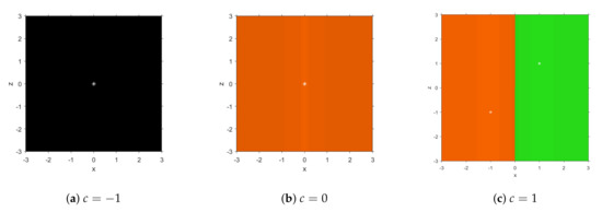
Figure 1. Dynamical planes of $P{M}_6$ method on $p\left(x\right)$, for different values of c.

Let us remark that, as by definition all the fixed points have equal components, they will always appear in the bisector of the first and third quadrants of the dynamical plane. It can be observed that, when there are no real roots ($c<0$, Figure 1a), no other attracting element appears; when $c=0$, the only root is multiple and the convergence is linear, so there is global convergence to $x=0$, as can be seen in Figure 1b. In Figure 1c, the convergence to the roots is also observed to be global, their basins of attraction being two symmetrical half-planes, which is exactly the same behavior as Newton’s method on quadratic polynomials.

Moreover, let us remark that when $c>0$ (real simple roots case), there are not free critical points, as in this case the only possible performance of the method was the convergence to the roots. The reason for this behavior is that in each basin of attraction there must be a critical point; if the only critical points are the roots of that basin, then there is no other possible convergence.

Comparisons with Other Methods with Memory for Nonlinear Problems

Here we compare the stability of the proposed method with that of known $A{M}_5$ and $S{M}_{4.45}$ schemes. Firstly, we show their performances on quadratic polynomials: $P{M}_6$. The dynamical planes are plotted in the complex plane, by starting the iterative methods with memory with an initial value of the accelerating parameter of $-0.01$ om each case, for any initial guess $z\in \mathbb{C}$, defined in a mesh of $400\times 400$ points and with a maximum of 80 iterations.

As shown in Figure 2 and Figure 3, all three methods have been used to estimate the complex roots of the unity of second and third degrees. It can be observed that the performances with $P{M}_6$ and $A{M}_5$ were very similar for quadratic polynomials, showing global convergence, similar to that of Newton’s scheme.

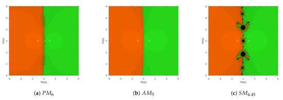
Figure 2. Complex dynamical planes of new and known methods on $x^2-1$.

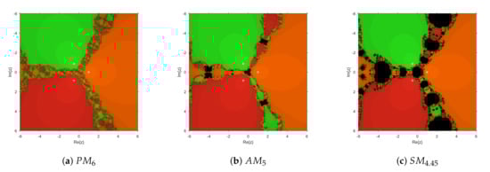
Figure 3. Complex dynamical planes of new and known methods on $x^3-1$.

However, this global convergence is held on cubic polynomials in the case of $P{M}_6$, but in case of $A{M}_5$, black areas of no convergence to the roots appear. Iterative method $S{M}_{4.45}$ shows these black regions both for quadratic and cubic polynomials, which are bigger in the cubic case.

This good performance of the set of converging initial estimations of proposed method $P{M}_6$ is also shown in the case of non-polynomial equations: let us notice the performances of all known and new methods on the complex rational function $f\left(z\right)={\displaystyle \frac{z^2-1}{z^2+1}}+1$, $z\in \mathbb{C}$ with a simple zero at $\xi =0$. The basins of attraction of the root appearing in Figure 4, being similar, are wider in case of $P{M}_6$ than for $A{M}_5$ or $S{M}_{4.45}$.

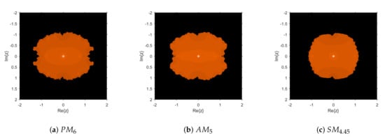
Figure 4. Complex dynamical planes of new and known methods on $f\left(z\right)={\displaystyle \frac{z^2-1}{z^2+1}}+1$ with $\xi =0$.

Additionally, in Figure 5 the basin of attraction of $\xi \approx 0.25753$, the simple root of $g\left(z\right)=z^2-exp\left(z\right)-3z+2$, is very wide in the case of $P{M}_6$, with small areas of no convergence to the root, in comparison with those of known methods $A{M}_5$ and $S{M}_{4.45}$.

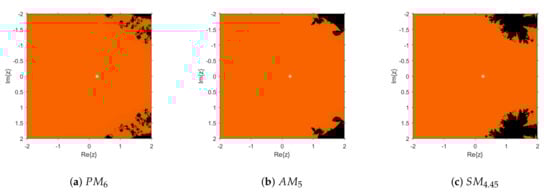
Figure 5. Complex dynamical planes of new and known methods on $z^2-exp\left(z\right)-3z+2$, with $\xi \approx 0.25753$.

Thus, it can be concluded that proposed method $P{M}_6$ had very stable performance, as in real and in complex spaces, both for polynomial and non-polynomial functions, in the scalar case. In spite of having the same accelerating parameter as the $A{M}_5$ method, the new scheme has proven to be better than known ones in terms of order of convergence and also in terms of stability. In the next section, its numerical performance on nonlinear systems of different sizes is demonstrated.

5. Numerical Experiments

This section presents the validity of the proposed scheme with memory on some numerical problems. The proposed method (22) was applied to numerical problems and compared with other existing techniques with memory [15,18], presented as $A{M}_5$ and $S{M}_{4.45}$, respectively. In all numerical problems, initially the parameter $\beta =B^{\left(0\right)}=-0.01I$, where I is the identity matrix, and for method $S{M}_{4.45}$, another parameter $c=-0.01$ was considered. All the numerical tests were conducted by using Mathematica 10, with 400 multiple precision digits of mantissa. For all the examples, we have included in the respective tables the following information: $\parallel x^{(j+1)}-x^{\left(j\right)}\parallel$; $j=0,1,2$; the residual $\parallel F\left(x^{\left(j\right)}\right)\parallel$ at $j=0,1,2$; approximated computational order of convergence (ACOC) denoted as $\rho$ [29]

$$\rho =\frac{ln\frac{\parallel x^{(j+1)}-x^{\left(j\right)}\parallel }{\parallel x^{\left(j\right)}-x^{(j-1)}\parallel }}{ln\frac{\parallel x^{\left(j\right)}-x^{(j-1)}\parallel }{\parallel x^{(j-1)}-x^{(j-2)}\parallel }},foreachj=2,3,\dots ;$$

(27)

and $CPU-time$.

Further on, the iterative procedure was stopped after three iterations and problems were tested on three different initial values. Notice that the meaning of $b(\pm a)$ is $b\times {10}^{\pm a}$ in all the tables.

Example 1.

Consider the following system of nonlinear equations in four unknown variables:

$$\begin{array}{cc}\hfill & x_2{x}_3+\left(x_2+x_3\right)x_4=0,\hfill \\ \hfill & x_2{x}_3+\left(x_2+x_3\right)x_4=0,\hfill \\ \hfill & x_1{x}_3+\left(x_1+x_3\right)x_4=0,\hfill \\ \hfill & x_1{x}_2+x_3{x}_2+x_1{x}_3=1.\hfill \end{array}$$

(28)

The approximate solution is ${(0.57735,0.57735,0.57735,-0.28867)}^T$. Table 1 depicts that the proposed scheme with all different initial guesses converged to a solution much faster than the methods $A{M}_5$ and $S{M}_{4.45}$. Clearly, the residual error, functional error and computational time of proposed method $P{M}_6$ were superior to those of $A{M}_5$ and $S{M}_{4.45}$.

Table 1. Convergence behavior of the schemes for Example 1.

${\mathit{x}}^{\left(0\right)}$	$\mathbf{Schemes}$	$\left|\right|{\mathit{x}}^{\left(1\right)}-{\mathit{x}}^{\left(0\right)}\left|\right|$	$\left|\right|{\mathit{x}}^{\left(2\right)}-{\mathit{x}}^{\left(1\right)}\left|\right|$	$\left|\right|{\mathit{x}}^{\left(3\right)}-{\mathit{x}}^{\left(2\right)}\left|\right|$	$\left|\right|\mathit{F}\left({\mathit{x}}^{\left(1\right)}\right)\left|\right|$	$\left|\right|\mathit{F}\left({\mathit{x}}^{\left(2\right)}\right)\left|\right|$	$\left|\right|\mathit{F}\left({\mathit{x}}^{\left(3\right)}\right)\left|\right|$	$\mathit{\rho }$	$\mathbf{CPU}-\mathbf{Time}$
$\left[\begin{array}{c}1\\ ⋮\\ 1\end{array}\right]$	$P{M}_6$	$8.4(-1)$	$2.7(-11)$	$1.0(-70)$	$1.8(-1)$	$5.4(-11)$	$2.1(-70)$	$6.040$	$0.422$
	$A{M}_5$	$2.1(-1)$	$1.7(-7)$	$2.4(-40)$	$4.6(-1)$	$3.5(-7)$	$4.9(-40)$	$5.395$	$0.549$
	$S{M}_{4.45}$	$7.9(-2)$	$1.3(-8)$	$6.9(-42)$	$1.7(-1)$	$2.7(-8)$	$1.4(-41)$	$4.917$	$0.577$
$\left[\begin{array}{c}0.5\\ ⋮\\ 0.5\end{array}\right]$	$P{M}_6$	$1.6(-3)$	$1.9(-24)$	$2.4(-152)$	$3.2(-3)$	$3.8(-24)$	$4.7(-152)$	$6.112$	$0.626$
	$A{M}_5$	$1.5(-2)$	$4.8(-16)$	$5.7(-86)$	$3.0(-2)$	$9.6(-16)$	$1.1(-85)$	$5.176$	$1.641$
	$S{M}_{4.45}$	$3.6(-4)$	$2.2(-21)$	$1.8(-99)$	$7.2(-4)$	$4.3(-21)$	$3.6(-99)$	$4.534$	$26.58$
$\left[\begin{array}{c}0.4\\ ⋮\\ 0.4\end{array}\right]$	$P{M}_6$	$3.3(-2)$	$1.6(-14)$	$8.3(-91)$	$6.4(-2)$	$3.1(-14)$	$1.7(-90)$	$6.185$	$0.532$
	$A{M}_5$	$1.3(-1)$	$5.1(-10)$	$1.9(-54)$	$2.5(-1)$	$1.0(-9)$	$3.7(-54)$	$5.282$	$0.621$
	$S{M}_{4.45}$	$1.6(-1)$	$2.1(-8)$	$8.5(-42)$	$3.1(-1)$	$4.3(-8)$	$1.7(-41)$	$4.859$	$0.682$

Example 2.

Another $200\times 200$ system of nonlinear equations defined as:

$$\begin{array}{cc}\hfill & x_i{x}_{i+1}-1=0,\hfill \\ \hfill & x_n{x}_1-1=0,i=1,2,\cdots ,n=200.\hfill \end{array}$$

(29)

The exact solution of this problem is ${(1,1,\cdots ,1)}^T.$ This system of nonlinear equations was examined on initial guesses ${(1.1,\cdots ,1.1)}^T$, ${(0.3,\cdots ,0.3)}^T$ and ${(0.8,\cdots ,0.8)}^T$; and results are shown in Table 2. The proposed technique performed better than existing scheme $A{M}_5$, whereas scheme $S{M}_{4.45}$ diverged for initial guess ${(0.3,\cdots ,0.3)}^T$. In the case of a large nonlinear system of equations, the proposed methods demonstrated an efficient order of convergence and short CPU time when compared with other schemes.

Table 2. Convergence behavior of schemes for Example 2.

${\mathit{x}}^{\left(0\right)}$	$\mathbf{Schemes}$	$\left|\right|{\mathit{x}}^{\left(1\right)}-{\mathit{x}}^{\left(0\right)}\left|\right|$	$\left|\right|{\mathit{x}}^{\left(2\right)}-{\mathit{x}}^{\left(1\right)}\left|\right|$	$\left|\right|{\mathit{x}}^{\left(3\right)}-{\mathit{x}}^{\left(2\right)}\left|\right|$	$\left|\right|\mathit{F}\left({\mathit{x}}^{\left(1\right)}\right)\left|\right|$	$\left|\right|\mathit{F}\left({\mathit{x}}^{\left(2\right)}\right)\left|\right|$	$\left|\right|\mathit{F}\left({\mathit{x}}^{\left(3\right)}\right)\left|\right|$	$\mathit{\rho }$	$\mathbf{CPU}-\mathbf{Time}$
$\left[\begin{array}{c}1.1\\ ⋮\\ 1.1\end{array}\right]$	$P{M}_6$	$2.9(-4)$	$6.4(-29)$	$7.3(-177)$	$5.8(-4)$	$1.3(-28)$	$1.5(-176)$	$6.000$	$143.215$
	$A{M}_5$	$3.2(-3)$	$5.1(-19)$	$5.2(-98)$	$6.4(-3)$	$1.0(-18)$	$1.0(-97)$	$5.000$	$313.076$
	$S{M}_{4.45}$	$1.8(-4)$	$3.4(-22)$	$2.8(-101)$	$3.5(-4)$	$6.9(-22)$	$5.6(-101)$	$4.465$	$180.219$
$\left[\begin{array}{c}0.3\\ ⋮\\ 0.3\end{array}\right]$	$P{M}_6$	$7.5$	$4.2(-3)$	$6.4(-22)$	$19.0$	$8.5(-3)$	$1.3(-21)$	$6.000$	$107.329$
	$A{M}_5$	$3.9$	$3.2(-3)$	$5.3(-19)$	$6.8$	$6.4(-3)$	$1.1(-18)$	$5.000$	$120.001$
	$S{M}_{4.45}$	d	d	d	d	d	d	d	d
$\left[\begin{array}{c}0.8\\ ⋮\\ 0.8\end{array}\right]$	$P{M}_6$	$1.0(-2)$	$1.1(-19)$	$2.1(-121)$	$2.0(-2)$	$2.2(-19)$	$4.3(-121)$	$5.999$	$92.843$
	$A{M}_5$	$4.0(-2)$	$1.7(-13)$	$2.1(-70)$	$8.1(-2)$	$3.4(-13)$	$4.1(-70)$	$5.000$	$93.905$
	$S{M}_{4.45}$	$3.3(-3)$	$3.0(-16)$	$2.5(-75)$	$6.5(-3)$	$5.9(-16)$	$5.0(-75)$	$4.529$	$191.609$

(d: stands for the divergent).

Example 3.

Next, we consider the transcendental system of equations shown below

$$-2\sum _{j=1}^{100}{x}_j^2+2x_j^2+{tan}^{-1}\left(x_i\right)+1=0,i=1,2,\dots ,100.$$

(30)

This problem has an approximated solution of ${(0.0736323\cdots ,0.0736323\cdots ,\cdots ,0.0736323\cdots )}^T$. The performance of the proposed method was better than those of the other methods ones, as shown in Table 3.

Table 3. Convergence behavior of schemes for Example 3.

${\mathit{x}}^{\left(0\right)}$	$\mathbf{Schemes}$	$\left|\right|{\mathit{x}}^{\left(1\right)}-{\mathit{x}}^{\left(0\right)}\left|\right|$	$\left|\right|{\mathit{x}}^{\left(2\right)}-{\mathit{x}}^{\left(1\right)}\left|\right|$	$\left|\right|{\mathit{x}}^{\left(3\right)}-{\mathit{x}}^{\left(2\right)}\left|\right|$	$\left|\right|\mathit{F}\left({\mathit{x}}^{\left(1\right)}\right)\left|\right|$	$\left|\right|\mathit{F}\left({\mathit{x}}^{\left(2\right)}\right)\left|\right|$	$\left|\right|\mathit{F}\left({\mathit{x}}^{\left(3\right)}\right)\left|\right|$	$\mathit{\rho }$	$\mathbf{CPU}-\mathbf{Time}$
$\left[\begin{array}{c}0.3\\ ⋮\\ 0.3\end{array}\right]$	$P{M}_6$	$6.6(-2)$	$2.2(-8)$	$4.6(-44)$	$2.0$	$6.3(-7)$	$1.3(-42)$	$5.511$	$638.578$
	$A{M}_5$	$8.4(-2)$	$7.6(-7)$	$3.9(-31)$	$2.5$	$2.1(-5)$	$1.1(-29)$	$3.558$	$726.233$
	$S{M}_{4.45}$	$5.2(-1)$	$8.6(-3)$	$3.7(-10)$	$23.0$	$2.4(-1)$	$1.0(-8)$	$4.134$	$759.5$
$\left[\begin{array}{c}0.1\\ ⋮\\ 0.1\end{array}\right]$	$P{M}_6$	$7.4(-4)$	$5.7(-20)$	$2.9(-98)$	$2.1(-2)$	$1.6(-18)$	$8.1(-97)$	$4.859$	$677.171$
	$A{M}_5$	$2.7(-3)$	$3.5(-14)$	$1.4(-59)$	$7.6(-2)$	$9.8(-13)$	$4.0(-58)$	$4.167$	$685.561$
	$S{M}_{4.45}$	$2.4(-3)$	$1.4(-12)$	$9.7(-54)$	$6.9(-2)$	$4.1(-11)$	$2.7(-52)$	$4.461$	$736.844$
$\left[\begin{array}{c}0.5\\ ⋮\\ 0.5\end{array}\right]$	$P{M}_6$	$5.4(-1)$	$1.0(-4)$	$4.4(-19)$	$21.0$	$2.9(-2)$	$1.2(-17)$	$5.653$	$897.173$
	$A{M}_5$	$5.5(-1)$	$2.5(-3)$	$2.5(-14)$	$22.0$	$7.1(-3)$	$7.1(-13)$	$4.694$	$809.123$
	$S{M}_{4.45}$	$1.4$	$1.3(-1)$	$4.5(-5)$	$86.0$	$3.9$	$1.3(-3)$	$3.352$	$1204.64$

Example 4.

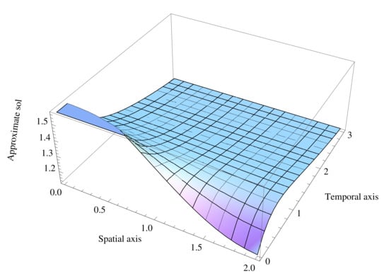
We have tested the proposed method on another well-known nonlinear problem Fisher’s equation [30] which has many applications in chemistry, heat and mass transfer, biology and ecology. Basically, it determines the process of interaction between diffusion and reaction. This nonlinear problem with homogeneous Neumann’s boundary conditions and diffusion coefficient D can be defined as:

$$\begin{array}{cc}\hfill & u_t=D{u}_{xx}+u(1-u)=0,\hfill \\ \hfill & u(x,0)=1.5+0.5cos\left(\pi x\right),0\le x\le 1,\hfill \\ \hfill & u_x(0,t)=0,\forall t\ge 0,\hfill \\ \hfill & u_x(1,t)=0,\forall t\ge 0.\hfill \end{array}$$

(31)

Applying the finite difference discreitization on the Equation (31) leads to a system of nonlinear equations. Suppose $w_{i,j}=u(x_i,t_j)$ is its approximate solution at the grid points of the mesh. Let M and N be the numbers of steps in x and t directions, and h and k be the respective step sizes. Use central difference to approximate the second order partial derivative $u_{xx}(x_i,t_j)=(w_{i+1,j}-2w_{i,j}+w_{i-1,j})/h^2$; backward difference approximation for the first-order derivative with respect to "t" as $u_t(x_i,t_j)=(w_{i,j}-w_{i,j-1})/k$; and forward difference for first order derivative with respect to x as $u_x(x_i,t_j)=(w_{i+1,j}-w_{i,j})/\left(h\right)$. The solution of the system is obtained by taking steps along x-axis, $M=21$, and t-axis, $N=21$, which form a nonlinear system of size 400, with the initial vector $x^{\left(0\right)}={(i/{(M-1)}^2)}^T,i=1,2,\dots ,M-1$. The results have been computed by different methods and are shown in Table 4. It can be noticed that the lowest execution time and residual error at the third iteration correspond to the proposed method $P{M}_6$. Moreover, the approximate solution has been plotted in Figure 6.

Table 4. Convergence behavior of schemes for Example 4.

$\mathbf{Schemes}$	$\left|\right|{\mathit{x}}^{\left(1\right)}-{\mathit{x}}^{\left(0\right)}\left|\right|$	$\left|\right|{\mathit{x}}^{\left(2\right)}-{\mathit{x}}^{\left(1\right)}\left|\right|$	$\left|\right|{\mathit{x}}^{\left(3\right)}-{\mathit{x}}^{\left(2\right)}\left|\right|$	$\left|\right|\mathit{F}\left({\mathit{x}}^{\left(1\right)}\right)\left|\right|$	$\left|\right|\mathit{F}\left({\mathit{x}}^{\left(2\right)}\right)\left|\right|$	$\left|\right|\mathit{F}\left({\mathit{x}}^{\left(3\right)}\right)\left|\right|$	$\mathit{\rho }$	$\mathbf{CPU}-\mathbf{Time}$
$P{M}_6$	$2.8$	$1.5(-7)$	$1.9(-51)$	$2.4\left(2\right)$	$3.9(-5)$	$8.9(-49)$	$6.0413$	$1333.85$
$A{M}_5$	$2.7$	$5.0(-6)$	$3.0(-35)$	$1.9\left(2\right)$	$9.2(-5)$	$1.3(-32)$	$5.0929$	$1415.90$
$S{M}_{4.45}$	$4.9$	$5.0(-5)$	$5.3(-27)$	$5.7\left(2\right)$	$1.5(-2)$	$2.6(-24)$	$4.3948$	$3606.19$

Figure 6. Approximated Solution for Fisher’s Equation $t\in [0,3]$.

6. Conclusions

The number of iterative schemes with memory for solving multidimensional problems is low, in part due to the difficulty of the task. Additionally, it is in part due to the lack of efficiency of the resulting method, if the usual techniques employed in the design of scalar methods with memory are employed as high-degree interpolation polynomials. With the procedure used, the iterative expression of the scheme with memory remains simple, and the order of the original method is increased by $50\%$. Thus, the efficiency is highly improved. Moreover it has been proven, by means of the associated multidimensional discrete dynamical system, that it is a very stable scheme with wide basins of attraction and global convergence on quadratic polynomials. Its performance on other nonlinear functions was also found to be very stable in comparison with other known schemes. The numerical tests confirmed these results, even for large nonlinear systems and applied problems, such as Fisher’s partial differential equation.

References

- Burden, R.L.; Faires, J.D. Numerical Analysis; PWS Publishing Company: Boston, MA, USA, 2001. [Google Scholar]
- Grosan, C.; Abraham, A. A new approach for solving nonlinear equations systems. IEEE Trans. Syst. Man Cybernet Part A Syst. Hum. 2008, 38, 698–714. [Google Scholar] [CrossRef]
- Moré, J.J. A collection of nonlinear model problems. In Computational Solution of Nonlinear Systems of Equations, Lectures in Applied Mathematics; Allgower, E.L., Georg, K., Eds.; American Mathematical Society: Providence, RI, USA, 1990; Volume 26, pp. 723–762. [Google Scholar]
- Tsoulos, I.G.; Stavrakoudis, A. On locating all roots of systems of nonlinear equations inside bounded domain using global optimization methods. Nonlinear Anal. Real World Appl. 2010, 11, 2465–2471. [Google Scholar] [CrossRef]
- Ortega, J.M.; Rheinboldt, W.C. Iterative Solution of Nonlinear Equations in Several Variables; Academic Press: New York, NY, USA, 1970. [Google Scholar]
- Samanskii, V. On a modification of the Newton method. Ukrain. Math. 1967, 19, 133–138. [Google Scholar]
- Traub, J.F. Iterative Methods for the Solution of Equations; Prentice-Hall: Englewood Cliffs, NJ, USA, 1964. [Google Scholar]
- Petković, M.S.; Neta, B.; Petkovixcx, L.D.; Džunixcx, J. Multipoint Methods for the Solution of Nonlinear Equations; Elsevier: Amsterdam, The Netherlands, 2012. [Google Scholar]
- Cordero, A.; Lotfi, T.; Bakhtiari, P.; Torregrosa, J.R. An efficient two-parametric family with memory for nonlinear equations. Numer. Algorithms 2015, 68, 323–335. [Google Scholar] [CrossRef] [Green Version]
- Wang, X.; Zhang, T.; Qin, Y. Efficient two-step derivative-free iterative methods with memory and their dynamics. Int. J. Comput. Math. 2016, 93, 1423–1446. [Google Scholar] [CrossRef]
- Cordero, A.; Lotfi, T.; Torregrosa, J.R.; Assari, P.; Taher-Khani, S. Some new bi-accelerator two-point method for solving nonlinear equations. J. Comput. Appl. Math. 2016, 35, 251–267. [Google Scholar] [CrossRef]
- Bakhtiari, P.; Cordero, A.; Lotfi, T.; Mahdiani, K.; Torregrosa, J.R. Widening basins of attraction of optimal iterative methods for solving nonlinear equations. Nonlinear Dyn. 2017, 87, 913–938. [Google Scholar] [CrossRef]
- Howk, C.L.; Hueso, J.L.; Martínez, E.; Teruel, C. A class of efficient high-order iterative methods with memory for nonlinear equations and their dynamics. Math. Meth. Appl. Sci. 2018, 41, 7263–7282. [Google Scholar] [CrossRef]
- Sharma, J.R.; Arora, H. Efficient higher order derivative-free multipoint methods with and without memory for systems of nonlinear equations. Int. J. Comput. Math. 2018, 95, 920–938. [Google Scholar] [CrossRef]
- Petkovíc, M.S.; Sharma, J.R. On some efficient derivative-free iterative methods with memory for solving systems of nonlinear equations. Numer. Algor. 2016, 71, 457–474. [Google Scholar] [CrossRef]
- Narang, M.; Bathia, S.; Alshomrani, A.S.; Kanwar, V. General efficient class of Steffensen type methods with memory for solving systems on nonlinear equations. Comput. Appl. Math. 2019, 352, 23–39. [Google Scholar] [CrossRef]
- Cordero, A.; Maimó, J.G.; Torregrosa, J.R.; Vassileva, M.P. Iterative methods with memory for solving systems of nonlinear equations using a second order approximation. Mathematics 2019, 7, 1069. [Google Scholar] [CrossRef] [Green Version]
- Chicharro, F.I.; Cordero, A.; Garrido, N.; Torregrosa, J.R. On the improvement of the order of convergence of iterative methods for solving nonlinear systems by means of memory. Appl. Math. Lett. 2020, 104. [Google Scholar] [CrossRef]
- Campos, B.; Cordero, A.; Torregrosa, J.R.; Vindel, P. A multidimensional dynamical approach to iterative methods with memory. Appl. Math. Comput. 2015, 271, 701–715. [Google Scholar] [CrossRef] [Green Version]
- Campos, B.; Cordero, A.; Torregrosa, J.R.; Vindel, P. Stability of King’s family of iterative methods with memory. Comput. Appl. Math. 2017, 318, 504–514. [Google Scholar] [CrossRef] [Green Version]
- Choubey, N.; Cordero, A.; Jaiswal, J.P.; Torregrosa, J.R. Dynamical techniques for analyzing iterative schemes with memory. Complexity 2018, 2018. [Google Scholar] [CrossRef]
- Chicharro, F.I.; Cordero, A.; Garrido, N.; Torregrosa, J.R. Stability and applicability of iterative methods with memory. J. Math. Chem. 2019, 57, 1282–1300. [Google Scholar] [CrossRef]
- Chicharro, F.I.; Cordero, A.; Garrido, N.; Torregrosa, J.R. On the choice of the best members of the Kim family and the improvement of its convergence. Math. Meth. Appl. Sci. 2020, 43, 8051–8066. [Google Scholar] [CrossRef]
- Chicharro, F.I.; Cordero, A.; Garrido, N.; Torregrosa, J.R. Impact on stability by the use of memory in Traub-type schemes. Mathematics 2020, 8, 274. [Google Scholar] [CrossRef] [Green Version]
- Cordero, A.; Hueso, J.L.; Martínez, E.; Torregrosa, J.R. A modified Newton-Jarratt’s composition. Numer. Alg. 2010, 5, 87–99. [Google Scholar] [CrossRef]
- Blanchard, P. Complex Analytic Dynamics on the Riemann Sphere. Bull. AMS 1984, 11, 85–141. [Google Scholar] [CrossRef] [Green Version]
- Robinson, R.C. An Introduction to Dynamical Systems, Continous and Discrete; American Mathematical Society: Providence, RI, USA, 2012. [Google Scholar]
- Chicharro, F.I.; Cordero, A.; Torregrosa, J.R. Drawing dynamical and parameters planes of iterative families and methods. Sci. World 2013, 2013. [Google Scholar] [CrossRef] [PubMed]
- Cordero, A.; Torregrosa, J.R. Variants of Newton’s method using fifth order quadrature formulas. Appl. Math. Comput. 2007, 190, 686–698. [Google Scholar] [CrossRef]
- Sauer, T. Numerical Analysis, 2nd ed.; Pearson: Boston, MA, USA, 2012. [Google Scholar]
Publisher’s Note: MDPI stays neutral with regard to jurisdictional claims in published maps and institutional affiliations. |
© 2021 by the authors. Licensee MDPI, Basel, Switzerland. This article is an open access article distributed under the terms and conditions of the Creative Commons Attribution (CC BY) license (https://creativecommons.org/licenses/by/4.0/).