Feedforward of Measurable Disturbances to Improve Multi-Input Feedback Control

Abstract

The availability of multiple inputs (plants) can improve output performance by conveniently allocating the control bandwidth among them. Beyond that, the intervention of only the useful plants at each frequency implies the minimum control action at each input. Secondly, in single input control, the addition of feedforward loops from measurable external inputs has been demonstrated to reduce the amount of feedback and, subsequently, palliate its sideband effects of noise amplification. Thus, one part of the action calculated by feedback is now provided by feedforward. This paper takes advantage of both facts for the problem of robust rejection of measurable disturbances by employing a set of control inputs; a previous work did the same for the case of robust reference tracking. Then, a control architecture is provided that includes feedforward elements from the measurable disturbance to each control input and feedback control elements that link the output error to each control input. A methodology is developed for the robust design of the named control elements that distribute the control bandwidth among the cheapest inputs and simultaneously assures the prescribed output performance to correct the disturbed output for a set of possible plant cases (model uncertainty). The minimum necessary feedback gains are used to fight plant uncertainties at the control bandwidth, while feedforward gains achieve the nominal output response. Quantitative feedback theory (QFT) principles are employed. An example illustrates the method and its benefits versus a control architecture with only feedback control elements, which have much more gain beyond the control bandwidth than when feedforward is employed.

1. Introduction

Uncertainties such as nonmeasurable disturbances or unavoidable simplifications in plant modelling justify feedback control loops, which, by permanently supervising the output, can correct its deviation from the reference or track reference changes. Better performances of the output response are linked to larger control bandwidths, which are provided by larger gains of feedback controllers (magnitude frequency response). Limited actuator ranges usually constrain the bandwidth and performance. Even for unlimited linear ranges or very powerful actuators, sensor noise amplifications at the control inputs impose an important constraint to the bandwidth to avoid fatigue or even saturation of actuators (Horowitz [1] labelled this fact as ‘the cost of feedback’). With this in mind, Quantitative Feedback Theory (QFT) [1,2,3] proposes incorporating feedforward controllers when external inputs are available (reference or measurable disturbance inputs [4]), reducing feedback gain to only that strictly necessary to compensate for the uncertainties. However, reduction of the feedback gain increases the feedforward gain to maintain a specific performance that is linked with the chosen closed-loop bandwidth. Then, the control action is univocally conditioned by the plant frequency response and the desired performance, but its convenient allocation between feedback and feedforward control actions can prevent excessive sensor noise amplification linked with feedback gain. These facts, which are common knowledge in single-input control, have not yet been fully exploited in multi-input control.

The use of multiple control inputs can undoubtedly improve closed-loop performance. A great variety of control structures and design methods are available in the scientific literature. Some works focused on widening the range of operating points for the output [5,6]. Other works focused on improving the output dynamic performance and simultaneously searched for a profitable combination of control inputs, branding them as input (valve) position control, mid-ranging control [7], or input resetting control [8]—their foundation [9] has inspired a set of works in the robust framework of QFT with the named missions of feedback and feedforward [10,11,12,13]. Thus, the robustly designed control elements determine the intervention or inhibition of plants (one for each input) along the frequency band. Let us consider the following facts: (i) some plants could provide the performance using less control action than others, p.e., those plants of larger magnitude, considering that magnitude dominance can change over the frequency band; (ii) plants that do not significantly contribute to the performance at certain frequencies are advised to be inhibited; (iii) the collaboration of productive plants can reduce the control action that is needed at their inputs—the virtual total control effort is divided among them. The frequency inhibition of unproductive plants is relevant for several reasons. It prevents high-frequency signals from exciting the actuators of plants that are useless at high frequencies [10]. Similarly, it also avoids inconvenient steady-state displacements of the operating point of plants that are useless at low frequencies [11]; applied works such as [14,15] highlight the relevance of resetting the steady-state points of high-frequency intervention plants. Finally, stability issues become critical when plants are out of phase, despite the fact that their magnitude contribution may be large and nearly the same [16,17]; Reference [12] presented an appropriate intervention of the magnitude frequency response of plants that were not minimum phase.

Structures with exclusive feedback controllers to the control inputs are the only possibility for rejection at the output of nonmeasurable disturbances. In [10,11], robust design methods of the feedback controllers distributed the frequency band among the most favourable plants to minimise the control action at each input (any number of inputs were possible) while achieving the desired performance of the output response. The control architecture of [10] allowed the collaboration of plants over the same frequency band while the architecture of [11] required separated work-bands in favour of an easier design method; unstable, nonminimum phase, or delayed plants were investigated in [12].

The reference tracking problem admits feedforward elements that can reduce the gain of feedback controllers to palliate noise amplification at control inputs [13]. Beyond that, the priority of the method in [13] was achieving correct distribution of the bandwidth among the inputs (plants) to obtain the performance using the minimum possible control action at each input.

The fact that disturbances are sometimes measurable variables opens the possibility of connecting feedforward paths to the control inputs, which can be exploited by this work. A control architecture with feedback and feedforward elements will be presented for robust disturbance rejection. The method will distribute the frequency band among the most favourable inputs (those that demand less control action). Finally, a robust design of the control elements will guarantee the prescribed performance and stability for a set of possible plant models. Feedforward will reduce feedback, reporting important benefits with regard to excessive sensor noise amplification at the control inputs that could saturate actuators and spoil the expected performance in feedback-only control structures. Whenever external disturbances are measurable, the contribution of this work can be of importance in a great variety of fields where multi-input control has been successfully applied. Remarkable application fields include bioprocesses [14,15], thermal systems [18], medical systems [19,20], scanner imaging [21,22], massive data storage devices [23,24], fuel engines [25] and electrical vehicles [26], robotics [27,28,29], and unmanned aerial vehicles [30].

2. Control Architecture and Robust Design Method

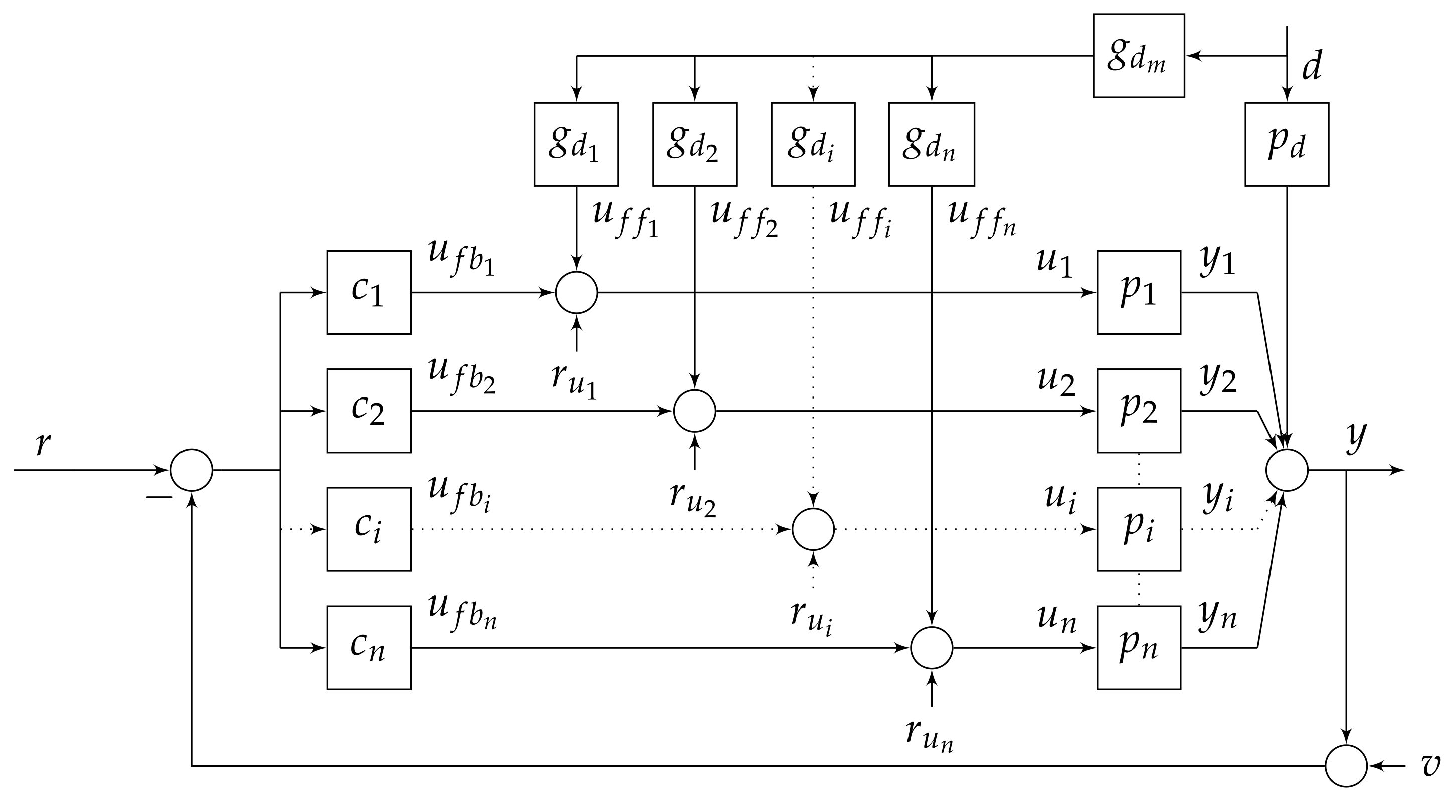
Figure 1 depicts the multiple-input single-output (MISO) system and the proposed control architecture. The y output deviation is modelled by the influence of $u_{i=1,\dots n}$ control inputs and a d disturbance input, achieving a vector of $(n+1)$ transfer functions (plants) $P\left(s\right)=[p_{i=1,\dots n}\left(s\right),p_d\left(s\right)]$. Let us consider a total number z of uncertain parameters in these dynamical models. By defining $q_l$ as a vector of those uncertain parameters in a set of all possible values of $\mathcal{Q}$ in ${\mathbb{R}}^z$, the MISO uncertain system can be formally defined as

$$\mathcal{P}=\{P(s;q_l):q_l\in \mathcal{Q}\}.$$

(1)

Henceforth, labels $p_i$ or $p_d$ denote plant models of delimited uncertainty.

An appropriate control must compensate for the output deviation from the constant reference, $e=r-y$, when a d disturbance occurs; reference tracking problems were discussed in [13]. Measurable disturbances are considered in the new design method. In such a case, the robust control specification is posed in the frequency domain as

$$\left|\frac{e}{d}\right|=\left|\frac{p_d+\left({\sum }_{i=1}^n{p}_i{g}_{d_i}\right)g_{d_m}}{1+{\sum }_{i=1}^n{p}_i{c}_i}\right|\le W_d;\forall P\in \mathcal{P},\forall \omega ,$$

(2)

where $W_d$ is an upper tolerance on the set of $|e/d|$ frequency responses.

As demonstrated in [10], when d is nonmeasurable (i.e., $g_{d_i}=g_{d_m}=0)$, the parallel structure of feedback controllers $c_{i=1,...,n}$ allows any distribution of frequencies for $u_{i=1,\dots n}$ participation to fulfil $|e/d|\le W_d$. Several $p_i$ plants could even collaborate over the same frequencies to reduce each $u_i$. On the other hand, a series structure of feedback controllers [11] obliges to a predefined location of plants inside the structure and requires separated frequency work-bands for the $u_i$ inputs. In spite of this, a method was provided to sort the plants and assign a convenient frequency band to each input to use the least $u_i$ possible.

Beyond those solutions, feedforward loops from the external input d to the control inputs $u_i$ are now being added. Individual elements $g_{d_i}$ allow the frequency band distribution for $u_i$ inputs with regard to feedforward tasks, while the feedforward master $g_{d_m}$ locates the responses e, taking advantage of the measurable information d; as long as there is a set of possible plants (1), there is a bunch of responses. The dispersion of frequency responses is constrained by feedback, which can be freely distributed among $u_i$ by controllers $c_i$. In summary, a total feedforward

$$l_{g_d}=\sum _{i=1}^n{l}_{g_{d_i}}=\left(\sum _{i=1}^n{p}_i{g}_{d_i}\right)g_{d_m}=p_{d_m}{g}_{d_m}$$

(3)

is contributed by individual feedforward channels $l_{g_{d_i}}$, which supply $u_{f{f}_i}$, and a total feedback

$$l_t=\sum _{i=1}^n{l}_i=\sum _{i=1}^n{p}_i{c}_i$$

(4)

is contributed by individual feedback loops $l_i$, which supply $u_{f{b}_i}$. Both components $u_{f{f}_i}$ and $u_{f{b}_i}$ build the control action $u_i$, which, for d handling, can be written and overbounded as

$$\left|\frac{u_i}{d}\right|=\left|\frac{u_{f{b}_i}}{d}+\frac{u_{f{f}_i}}{d}\right|=\left|-\frac{p_d+l_{g_d}}{1+l_t}{c}_i+g_{d_i}{g}_{d_m}\right|\le W_d|c_i|+|g_{d_i}{g}_{d_m}|;\forall P\in \mathcal{P},\forall \omega .$$

(5)

In SISO control ($i=n=1$), the desired performance for $e/d$ univocally fixes the only control action $u_1/d$, which can be distributed as desired between feedback and feedforward components. QFT prioritises feedforward to reduce as much feedback as possible and its said drawbacks; [4] provided a design solution inside a tracking error structure such as ours, which pursues the smallest $p_1{c}_1$ gain that guarantees the existence of $p_1{g}_d$ to meet (2); in this way, the amplification of sensor noise v at the control input $u_1$ that depends on $c_1$ gain is also reduced as much as possible. However, evaluating (5), a reduction of $u_{f{b}_1}/d$ occurs at the expense of an increase in $u_{f{f}_1}/d$, since $u_1$ is unique to provide the performance, i.e., the gain of $g_d=g_{d_1}{g}_{d_m}$ increases.

On the other hand, a multi-input availability offers many more possibilities. Let us note that despite the distribution between $l_t$ and $l_{g_d}$ that was selected to achieve the performance (2), infinite combinations of $l_i$ (4) and $l_{g{d}_i}$ (3) could build them. The goal is to find the solution that uses the set of smaller control inputs $u_i/d$. The authors of [13] provided a method for the problem of robust reference tracking ($r\ne \mathrm{constant}$). The key point was the more the gain of a plant, the less the need of control action to contribute to the performance, which foresaw the use of inputs towards plants with higher gains at each frequency.

In the current case, let us suppose a single input $u_i$ (plant $p_i$) participates in the disturbance rejection. If plant models are perfectly known, the control action $u_i=-p_d/p_i$ would cancel the d disturbance influence on the y output. Here, the whole set of plant uncertainties is being considered in the robust design. Then, the frequency response

$$k_i=\frac{p_{d,max}}{p_{i,min}},\forall P\in \mathcal{P},\forall \omega$$

(6)

is a rough approximation of the less favourable $u_i$ if only $p_i$ participates in the d disturbance rejection; $p_{i,min}$ is the plant $p_i$ of least magnitude at a particular $\omega$ inside the uncertain set $|p_i\left(j\omega \right)|$; and $p_{d,max}$ is the plant $p_d$ of largest magnitude at $\omega$ inside $|p_d\left(j\omega \right)|$.

Next, the $k_i$ frequency responses of all inputs $i=1,\dots ,n$ are compared at each frequency to decide which inputs are of sufficient interest for participation; those that yield the smallest $k_i$ magnitude are considered. At any frequency, the contribution of as many inputs as possible is desired, if it yields a total plant

$$p_{d_m}=\sum _{i=1}^n{p}_i{g}_{d_i},$$

(7)

with significantly greater magnitude than the individuals $p_i$ (let us advance that $g_{d_i}$ will be designed as filters with unitary gain at the pass band). Thus, the potential collaboration of plants would reduce individual feedforward actuations $|u_{f{f}_i}/d|$ because the virtual need of total feedforward $|\sum u_{f{f}_i}/d|\approx |p_d/p_{d_m}|$ would be significantly reduced. A two-in-two comparison of $k_i$ is advised. As a rule of thumb, a difference in $k_i\left(j\omega \right)$ magnitude greater than $20\log 2=6$ dB makes the plant associated with larger $k_i\left(j\omega \right)$ magnitude useless. When a plant cannot report benefits at a certain frequency, its disconnection is recommended to avoid useless signals reaching the actuators. A second relevant point is to check that the $k_i\left(j\omega \right)$ phase-shift of those plants that are likely to collaborate is less than ${90}^{\circ }$, since the vector sum of plants in the counter-phase would reduce the total magnitude of $p_{d_m}$ (7). The disconnection of useless plans in the counter-phase is a priority for stability issues [12].

The $k_i$ comparisons decide the smallest $u_i$ input at each frequency, i.e., the desired frequency band allocation among inputs. Then, the design of $g_{d_i}$ and $c_i$ must attain the planned distribution and, simultaneously, $g_{d_i}$, $c_i$, and $g_{d_m}$ must achieve the specification (2). The design method is described as follows: First, $g_{d_i}$ are designed as filters with unitary gain over the pass-band. This yields a convenient plant $p_{d_m}$ (7) that selects the most powerful $p_i$ plants at each frequency for feedforward tasks. Subsequently, feedback $l_t$ must reduce the influence of $p_{d_m}$ uncertainty in $|e/d|$ deviations around zero only to the extent that a master feedforward $g_{d_m}$ can further position the magnitude frequency responses inside tolerance $\pm W_d$. The required amount of feedback $l_t$ could be provided with several combinations of $c_i$, but the one according to the planned distribution will save the control action by using the most powerful plants at each frequency for feedback tasks too. The set of controllers $c_i$ are designed via loop-shaping of $l_i\left(j\omega \right)$ to satisfy the bounds ${\beta }_{l_i}\left(\omega \right)$ at a discrete set of frequencies $\Omega =\left\{\omega \right\}$. The QFT bounds ${\beta }_{l_i}$ translate the closed loop specification into terms of restrictions for $l_i=c_i{p}_i$ nominal at specific frequencies $\omega$ that are conveniently selected according to the plant and specifications; the bounds are depicted on a mod-arg plot [2,3]. During $l_i\left(j\omega \right)$ shaping, when it lies exactly on the bounds, it guarantees the minimum gain of the $c_i$ controller to achieve the specification by the whole set of plant cases. A sequential process between the $i=1,...,n$ loops is arbitrated. Thus, if at some point the controller $c_i$ is to be adjusted and the other controllers $c_{k\ne i}$ take known values in the sequence, the robust disturbance rejection specification (2) can be rewritten as

$$\left|\frac{e}{d}\right|=\left|\frac{p_d+g_{d_m}{p}_{d_m}}{1+{\sum }_{k\ne i}{p}_k{c}_k+p_i{c}_i}\right|\le W_d;\forall P\in \mathcal{P},\forall \omega ,$$

(8)

and their representative ${\beta }_{l_i}$ bounds can be computed by choosing $A=p_{d_m}$, $B=p_d$, $C=1+{\sum }_{k\ne i}{p}_k{c}_k$, $D=p_i$, $G=c_i$, $G_f=g_{d_m}$, and $W=W_d$ in the solution given to

$$\left|\frac{A{G}_f+B}{C+DG}\right|\le W$$

(9)

in [13]; this work provided the formulation to make the design of $c_i$ and $g_{d_m}$ independent. After the bound computation, the essence of loop-shaping is that $c_i$ reaches the necessary gain at the frequencies where the $p_i$ plant must work and filters (gain below 0 dB) those frequencies where $p_i$ must not work. Special attention must be paid to the frequencies where several inputs must collaborate. A detailed explanation of the global procedure is given in [10].

The full achievement of (2) ends with the design of the master feedforward $g_{d_m}$. The specification format can now be adapted to $\left|(A+BG)/(C+DG)\right|\le W$ of function gndbnds in the QFT toolbox [31]. By choosing $A=p_d$, $B=p_{d_m}$, $C=1+l_t$, $D=0$, $G=g_{d_m}$, and $W=W_d$, the regions that are permitted for $g_{d_m}$ on a mod-arg plot are determined; the loop-shaping of $g_{d_m}\left(j\omega \right)$ is conducted on these bounds.

Considering the whole set of external inputs, the output error responds to

$$e=-\frac{p_d+l_{g_d}}{1+l_t}d+\frac{1}{1+l_t}(r-v)-\sum _{i=1}^n\frac{p_i}{1+l_t}{r}_{u_i},$$

(10)

and the control inputs are

$$u_i=\left[-\frac{p_d+l_{g_d}}{1+l_t}{c}_i+g_{d_i}{g}_{d_m}\right]d+\frac{c_i}{1+l_t}(r-v)+\frac{(1+l_{-i})}{1+l_t}{r}_{u_i}-\sum _{k\ne i}\frac{c_i{p}_k}{1+l_t}{r}_{u_k},$$

(11)

where $l_{-i}=l_t-l_i$. Two benefits are mentioned. The availability of multiple inputs made it possible to select the intervention of the more favourable plants $p_i$ at each frequency to achieve $|e/d|<W_d$ using the minimum $|u_i/d|$. Individual feedforward $g_{d_i}$ and individual feedback $c_i$ either disconnected or not the commanded inputs at each frequency; integrators or derivators are recommended to connect or disconnect plants at low frequency to fully eliminate steady-state errors [13]. Further, $c_i$ and $g_{d_m}$ were in charge of providing $|e/d|<W_d$; let us recall that $g_{d_i}$ were filters of unitary gain at the pass-band. The use of feedforward $g_{d_m}$ allows reducing the amount of feedback $|c_i|$; in fact, the formal QFT method pursues the minimum set of $|c_i|$ for the existence of $g_{d_m}$. As $|c_i|$ reduces, $|u_i/v|$ (11) also reduces in comparison with $g_{d_m}=0$ solutions (feedback-only control structures are the only option when disturbances are nonmeasurable, as in [10,12]).

An additional flexibility of multi-input systems is the possibility of moving the system operating point $u_i(t=\infty )$ by changing the input resetting point $r_{u_i}\left(t\right)$ of the plants that do not work at low frequencies [9,12,32].

The output reference $r\left(t\right)$ is considered constant in the present work. For tracking control problems, feedforwarding $r\left(t\right)$ can achieve important benefits; a control architecture and design method were provided in [13].

3. Example

The following theoretical example illustrates the new method of designing feedback and feedforward elements. In addition to analysing how the specification of robust disturbance rejection is achieved with the minimum set of control actions, a comparison with a control structure with only feedback elements is conducted, proving the superiority of the feedback–feedforward structure. References [10,12] collected other examples with only feedback elements.

A system with two control inputs obeys the following models $y/u_i$, $i=1,2$, with parametric uncertainty:

$$\begin{array}{cccc}\hfill & p_1\left(s\right)=\frac{a_1}{{\left(\frac{a_2}{a_1}s+1\right)}^2},\hfill & \hfill a_1\in [1.60,2.40],& a_2\in [0.17,18.00];\hfill \\ \hfill & p_2\left(s\right)=\frac{b_1}{b_{2}s+1},\hfill & \hfill b_1\in [0.98,1.02],& b_2\in [0.33,1.00].\hfill \end{array}$$

(12)

The d disturbance input influence follows the uncertain parametric model $y/d$:

$$p_d\left(s\right)=\frac{c_1}{s+c_2},c_1\in [2.00,3.00],c_2\in [1.00,2.00].$$

(13)

Robust stability specifications

$$\left|T_i\left(j\omega \right)\right|=\left|\frac{l_i\left(j\omega \right)}{1+l_t\left(j\omega \right)}\right|\le W_{s_i},i=1,2;\forall P\in \mathcal{P},\forall \omega ,$$

(14)

seek minimum phase margins of ${40}^{\circ }$ for both feedback loops $i=1,2$ by taking

$$W_{s_i}=\left|\frac{0.5}{cos\left(\pi \right(180-PM)/360)}\right|,PM={40}^{\circ }.$$

(15)

Their representative bounds will delimit forbidden regions around the critical point that cannot be violated by $l_i=c_i{p}_i/(1+{\sum }_{j\ne i}{l}_j)$ at any $\omega$-frequency during loop-shaping [11,12,32]. These bounds can be computed with traditional CAD tools in the QFT toolbox [31].

The specification for the robust rejection of measurable d-disturbances (2) adopts the tolerance

$$W_d\left(\omega \right)={\left|\frac{0.2s}{{(0.5s+1)}^2}\right|}_{s=j\omega },$$

(16)

whose magnitude frequency response is plotted together with the magnitude frequency responses of plants in Figure 2a. The error tolerance $W_d\left(\omega \right)$ will allow reducing the feedback to zero as soon as possible over $\omega >4$. However, as $W_d\left(\omega \right)<\left|p_d\left(j\omega \right)\right|$, a small feedforward action will be needed at those frequencies. The problem arises when only feedback action is used, since feedback can never be neglected at high frequencies. Thus, a new specification

$$W_{dfb}\left(\omega \right)={\left|\frac{0.2s(0.1s+1)}{{(0.5s+1)}^2}\right|}_{s=j\omega }$$

(17)

is defined for the comparison of the new control architecture with the feedback-only architecture. Let us remark that time-domain performance will not be appreciatively altered between the use of (16) or (17) since their differences occur after the control bandwidth (see Figure 2a).

The set of discrete frequencies

$$\Omega =\{0.01,0.1,0.2,0.4,0.8,1,4,8,10,20\}\left[\mathrm{rad}/\mathrm{s}\right]$$

(18)

will be used for the assignment of working frequencies to inputs (plants) for bound calculations and to guide loop-shaping in the QFT framework. These have been selected considering the frequency response of plants and of the open-loop and closed-loop transfer functions.

3.1. Design Methodology

The frequency band allocation that minimises $u_i$ is founded on the $k_i$ frequency responses (6), which are depicted in Figure 3. The criteria argued in Section 2 advise that $p_1$ works over $\omega <0.2$ and $p_2$ works over $\omega >1.0$ since their respective $k_i$ magnitudes are the lesser over those frequencies. Additionally, the collaboration of both plants over $0.2\le \omega \le 1.0$ is advised since the difference between $k_i$-magnitudes is less than 6 dB, and the difference between $k_i$-phases is less than 90${}^{\circ }$.

Table 1. Frequency-band allocation that minimises $u_i$.

$\mathit{\omega }$	0.01	0.1	0.2	0.4	0.8	1	4	8	10	20
$p_1$	×	×	×	×	×	×
$p_2$			×	×	×	×	×	×	×	×

summarises all these conclusions.

According to the desired frequency band allocation (Table 1), the design of the individual feedforward elements yields

$$g_{d_1}\left(s\right)=\frac{1}{s+1},g_{d_2}\left(s\right)=\frac{s}{s+0.2}.$$

(19)

The low-pass filter $g_{d_1}$ attains a cut-off frequency of ${\omega }_c=1$, and the high-pass filter $g_{d_2}$ attains a cut-off frequency of ${\omega }_c=0.2$. The use of individual filters $g_{d_{i=1,2}}$ modifies the outcome plant $p_{d_m}$ (7) to be handled by feedback $c_{i=1,2}$ and the remaining feedforward $g_{d_m}$. Figure 2b proves how $p_{d_m}$ selects the more powerful part of plants $p_{i=1,2}$, which will minimise $u_{f{f}_i}$ to satisfy the performance specification (2) and (16).

For the design of feedback controllers $c_i$, the bounds ${\beta }_{l_i}$ that represent performance (2) and (16) and stability (14) and (15) specifications are computed. Then, each $l_i$ nominal, $l_{i_o}=p_{i_o}{c}_i$, is shaped to meet the bounds considering the frequency band allocation that minimises $u_{f{b}_i}$ (see Table 1). Figure 4 depicts the bounds and loop-shapings; nominal plants $p_{i_o}$ correspond to parameters $a=0.16,b=1.36,c=0.98,d=1.00$ in (12). The resulting controllers are

$$c_1\left(s\right)=\frac{1.575(s+0.08)}{s(s+0.12)(s+1.5)},c_2\left(s\right)=\frac{1.5(s+0.6)}{{(s+0.3)}^2}.$$

(20)

Finally, the bounds on the feedforward master are computed, and the loop-shaping (see Figure 4) yields

$$g_{d_m}\left(s\right)=\frac{-1.1849(s+0.1)(s+0.175)(s+2)}{(s+0.052)(s^2+0.8563s+0.2072)}.$$

(21)

If no feedforward loops are employed ($g_{d_1}=g_{d_2}=g_{d_m}=0$), feedback controllers $c_{i=1,2}$ should complete the whole job. In such a case, after computing the bounds that represent the specifications of robust disturbance rejection (2) and (17) and robust stability (14) and (15), the shaping of $l_{i_o}$, $i=1,2$, yields

$$c_1=\frac{108(s+0.1)}{s(s+10)(s+0.4)},c_2=\frac{964.49{(s+2.5)}^2(s+0.2)}{(s+74)(s+7.8)(s^2+0.45s+0.0625)}.$$

(22)

3.2. Analysis and Comparatives

Figure 5 shows several magnitude frequency responses of interest; the feedback-feedforward solution is depicted in blue and the feedback-only solution is in red; where applicable, several plant cases (12) are depicted.

In particular, closed-loop frequency responses of subplots (a) and (b) in Figure 5 prove the fulfilment of robust specifications on disturbance rejection and stability, respectively. A tight achievement of performance tolerance in the control bandwidth ($\omega \le 4$) can be noticed because some plant cases are close to or on the tolerance $W_d\left(\omega \right)$; to achieve it, observe how $l_{1_o}$ is onto ${\beta }_{l_1}$ at $\omega =\{0.01,0.1,0.2\}$ and $l_{2_o}$ onto ${\beta }_{l_2}$ at $\omega =\{0.2,0.4,0.8,1\}$ in Figure 4, which requires a relatively high order of the controllers (20) and (22). In addition, Table 1 planning has been executed successfully: $l_1$-$l_{g_1}$ of the feedback–feedforward solution and $l_1$ of the feedback-only solution work alongside the low-frequency band, and $l_2$-$l_{g_2}$ of feedback–feedforward and $l_2$ of feedback-only work alongside the high-frequency band (see subplots (e) and (f) in Figure 5).

The expected benefits of the above are using the minimum $|u_i/d|$ over $\omega \le 4$ (see subplot (g) in Figure 5). Regarding the frequency band distribution among plants, let us note, p.e., that if $p_2$ were forced to work at low frequency instead of $p_1$, $|u_2/d\left(j0\right)|$ would be $|p_1/p_2\left(j0\right)|$ larger than the current $|u_1/d\left(j0\right)|$. Regarding the tight achievement of bounds for each input design, it seeks the strictly necessary $|u_i/d|$ to achieve the specification; observe how $|u_1/d|$ along $\omega \le 1$ and $|u_2/d|$ along $0.2\le \omega \le 4$ are very similar for both solutions. The minimum effort in the control bandwidth pursues that $|u_i/v|$ can be reduced as soon as possible at high frequencies (see subplot (h) in Figure 5). However, the collaboration of feedback $l_i$ and feedforward $l_{g_i}$ to build $u_i/d$ yields smaller magnitudes $|l_i|$ than when only feedback intervenes (see subplot (e) in Figure 5). Then, feedback gains $|c_i|$ are smaller not only in the control bandwidth but also beyond the work-band of each input (see subplot (c) in Figure 5). The end effect $|u_1/v|$ over $\omega >1$ is smaller for the feedback–feedforward solution than for the feedback-only solution, and the same occurs for $|u_2/v|$ over $\omega >4$ (see subplot (h) in Figure 5). In fact, a huge noise amplification is expected at the second control input in the feedback-only solution.

Figure 6 shows the time-domain behaviour. External inputs are a unit step change of disturbance $d\left(t\right)$ at $t=1$ s and a sensor noise $v\left(t\right)$ that is built with a band-limited, white-noise source of Simulink® (power of 0.00005 and sample time of 0.01 s); the reference input $r\left(t\right)$ is constant and equal to zero. Blue and red colours distinguish the responses of feedback–feedforward and feedback-only solutions, respectively. Several plant cases are represented.

As expected, the output response $y\left(t\right)$ is built by the faster response $y_2\left(t\right)$ of the plant $p_2$, which works at high frequencies, and by the slower response $y_1\left(t\right)$ of the plant $p_1$, which progressively takes control of the steady-state. Ignoring the noise, the control actions $u_1\left(t\right)$ and $u_2\left(t\right)$, which command the plants $p_1$ and $p_2$, corroborate the same. Let us also remark how the input $u_2$, which does not work at steady-state, recovers the initial operating point $r_{u_2}=0$. Further, observe that $y\left(t\right)$ finally recovers the initial steady-state of zero. Both steady-state conditions $y=r$ and $u_2=r_{u_2}$ require an integrator in $c_1$ (20) and (22) and a differentiator in $g_{d_2}$ (19). Regarding the control actions, $u_i\left(t\right)$ is built with $u_{f{f}_i}\left(t\right)$ and $u_{f{b}_i}\left(t\right)$ in the feedback–feedforward solution, while $u_i\left(t\right)=u_{f{b}_i}\left(t\right)$ is built in the feedback-only solution. The main difference between both solutions is the $v\left(t\right)$ noise amplification at the output and, mainly, at the control inputs. The huge noise amplification at $u_2\left(t\right)$ of the feedback-only solution would cause fatigue of the actuator or might saturate it and spoil the theoretical performance. In such a case, a more conservative specification for disturbance rejection $e/d$ would be indicated in true-life control (higher tolerance $W_d$ in the control bandwidth). All these corroborate the superiority of feedback–feedforward schemes.

4. Conclusions

A new control architecture and design methodology has been proposed for the robust rejection of measurable disturbances when multiple control inputs are available to correct the output deviation. The multi-input character allowed selecting the most favourable plants (inputs) at each frequency to provide the performance. Thus, individual feedback and feedforward controllers to each input allowed distributing the control bandwidth as desired among the inputs; the allocation criterion was minimising the control action to provide the performance. Beyond that, the main benefit of the new structure is the presence of feedforward loops. This allowed reducing the amount of feedback and, consequently, the sensor noise amplification at the output and, mainly, at the control inputs. The advantages would be notorious in real-life systems, since excessive noise at actuators could sacrifice the achievement of the aggressive performance of the output. Finally, it is important to recall the robust character of the control system, which guaranteed the expected performance for a set of possible plant models.

References

1. Horowitz, I. Survey of quantitative feedback theory (QFT). Int. J. Robust Nonlinear Control. 2001, 11, 887–921. [Google Scholar] [CrossRef]
2. Houpis, C.; Rasmussen, S.; Garcia-Sanz, M. Quantitative Feedback Theory. Fundamentals and Applications; CRC Press Book: Boca Raton, FL, USA, 2006. [Google Scholar]
3. García-Sanz, M. Robust Control Engineering: Practical QFT Solutions; CRC Press: Boca Raton, FL, USA, 2017; pp. 1–556. [Google Scholar] [CrossRef]
4. Elso, J.; Gil-Martínez, M.; García-Sanz, M. Quantitative feedback-feedforward control for model matching and disturbance rejection. IET Control. Theory Appl. 2013, 7, 894–900. [Google Scholar] [CrossRef]
5. Reyes-Lúa, A.; Skogestad, S. Multiple-input single-output control for extending the steady-state operating range-use of controllers with different setpoints. Processes 2019, 7, 941. [Google Scholar] [CrossRef] [Green Version]
6. Reyes-Lúa, A.; Skogestad, S. Multi-input single-output control for extending the operating range: Generalized split range control using the baton strategy. J. Process. Control 2020, 91, 1–11. [Google Scholar] [CrossRef]
7. Hägglund, T. A feedforward approach to mid-ranging control. Control. Eng. Pract. 2021, 108, 104713. [Google Scholar] [CrossRef]
8. Sun, B.; Skogestad, S.; Lu, J.; Zhang, W. Dual SIMC-PI Controller Design for Cascade Implement of Input Resetting Control with Application. Ind. Eng. Chem. Res. 2018, 57, 6947–6955. [Google Scholar] [CrossRef]
9. Allison, B.J.; Ogawa, S. Design and tuning of valve position controllers with industrial applications. Trans. Inst. Meas. Control. 2003, 25, 3–16. [Google Scholar] [CrossRef]
10. Rico-Azagra, J.; Gil-Martínez, M.; Elso, J. Quantitative feedback control of multiple input single output systems. Math. Probl. Eng. 2014, 2014, 1–17. [Google Scholar] [CrossRef] [Green Version]
11. Gil-Martínez, M.; Rico-Azagra, J.; Elso, J. Frequency domain design of a series structure of robust controllers for multi-input single-output systems. Math. Probl. Eng. 2018, 2018. [Google Scholar] [CrossRef]
12. Gil-Martínez, M.; Rico-Azagra, J. Robust Feedback Control for Nonminimum Phase, Delayed, or Unstable Systems with Multiple Inputs. Math. Probl. Eng. 2020, 2020. [Google Scholar] [CrossRef]
13. Rico-Azagra, J.; Gil-Martínez, M. Feedforward for robust reference tracking in multi-input feedback control. IEEE Access 2021, 9, 92553–92567. [Google Scholar] [CrossRef]
14. Johnsson, O.; Sahlin, D.; Linde, J.; Lidén, G.; Hägglund, T. A mid-ranging control strategy for non-stationary processes and its application to dissolved oxygen control in a bioprocess. Control. Eng. Pract. 2015, 42, 89–94. [Google Scholar] [CrossRef]
15. Nájera, S.; Gil-Martínez, M.; Rico-Azagra, J. Dual-control of autothermal thermophilic aerobic digestion using aeration and solid retention time. Water 2017, 9, 426. [Google Scholar] [CrossRef] [Green Version]
16. Schroeck, S.J.; Messner, W.C.; McNab, R.J. On compensator design for linear time-invariant dual-input single-output systems. IEEE/ASME Trans. Mechatron. 2001, 6, 50–57. [Google Scholar] [CrossRef]
17. Alvarez-Ramirez, J.; Velasco, A.; Fernandez-Anaya, G. A note on the stability of habituating process control. J. Process. Control. 2004, 14, 939–945. [Google Scholar] [CrossRef]
18. Zotică, C.; Pérez-Piñeiro, D.; Skogestad, S. Supervisory control design for balancing supply and demand in a district heating system with thermal energy storage. Comput. Chem. Eng. 2021, 149, 107306. [Google Scholar] [CrossRef]
19. Van Heusden, K.; Ansermino, J.M.; Dumont, G.A. Robust MISO control of propofol-remifentanil anesthesia guided by the neurosense Monitor. IEEE Trans. Control. Syst. Technol. 2018, 26, 1758–1770. [Google Scholar] [CrossRef]
20. Eskandari, N.; van Heusden, K.; Dumont, G.A. Extended habituating model predictive control of propofol and remifentanil anesthesia. Biomed. Signal Process. Control 2020, 55, 101656. [Google Scholar] [CrossRef]
21. Soltani Bozchalooi, I.; Youcef-Toumi, K. Multi-actuation and PI control: A simple recipe for high-speed and large-range atomic force microscopy. Ultramicroscopy 2014, 146, 117–124. [Google Scholar] [CrossRef]
22. Soltani Bozchalooi, I.; Careaga Houck, A.; AlGhamdi, J.; Youcef-Toumi, K. Design and control of multi-actuated atomic force microscope for large-range and high-speed imaging. Ultramicroscopy 2016, 160, 213–224. [Google Scholar] [CrossRef]
23. Li, H.; Du, C.; Wang, Y. Optimal reset control for a dual-stage actuator system in HDDs. IEEE/ASME Trans. Mechatron. 2011, 16, 480–488. [Google Scholar] [CrossRef]
24. Zheng, J.; Fu, M. A unified dual-stage actuator control scheme for track seeking and following in hard disk drives. IET Control Theory Appl. 2012, 6, 1468–1477. [Google Scholar] [CrossRef]
25. Jade, S.; Larimore, J.; Hellstrom, E.; Jiang, L.; Stefanopoulou, A.G. Enabling large load transitions on multicylinder recompression HCCI engines using fuel governors. In Proceedings of the American Control Conference, Washington, DC, USA, 17–19 June 2013; pp. 4423–4428. [Google Scholar] [CrossRef]
26. Wu, J.; Liang, J.; Ruan, J.; Zhang, N.; Walker, P. A robust energy management strategy for EVs with dual input power-split transmission. Mech. Syst. Signal Process. 2018, 111, 442–455. [Google Scholar] [CrossRef]
27. Ma, Z.; Poo, A.N.; Ang, M.H., Jr.; Hong, G.S.; See, H.H. Design and control of an end-effector for industrial finishing applications. Robot. Comput.-Integr. Manuf. 2018, 53, 240–253. [Google Scholar] [CrossRef]
28. Nainer, C.; Furci, M.; Seuret, A.; Zaccarian, L.; Franchi, A. Hierarchical Control of the Over-Actuated ROSPO Platform via Static Input Allocation. IFAC-PapersOnLine 2017, 50, 12698–12703. [Google Scholar] [CrossRef]
29. Schneider, U.; Olofsson, B.; Sörnmo, O.; Drust, M.; Robertsson, A.; Hägele, M.; Johansson, R. Integrated approach to robotic machining with macro/micro-actuation. Robot. Comput.-Integr. Manuf. 2014, 30, 636–647. [Google Scholar] [CrossRef]
30. Haus, T.; Ivanovic, A.; Car, M.; Orsag, M.; Bogdan, S. Mid-Ranging Control Concept for a Multirotor UAV with Moving Masses. In Proceedings of the MED 2018-26th Mediterranean Conference on Control and Automation, Zadar, Croatia, 19–22 June 2018; pp. 339–344. [Google Scholar] [CrossRef]
31. Borghesani, C.; Chait, Y.; Yaniv, O. Quantitative Feedback Theory Toolbox. For Use with Matlab, 2nd ed.; Terasoft: San Diego, CA, USA, 2002. [Google Scholar]
32. Rico-Azagra, J.; Gil-Martínez, M.; Rico, R.; Maisterra, P. QFT bounds for robust stability specifications defined on the open-loop function. Int. J. Robust Nonlinear Control 2018, 28, 1116–1125. [Google Scholar] [CrossRef]
Figure 1. Feedback–feedforward control structure for robust rejection of measurable disturbances in multi-input systems.
Mathematics 09 02114 g001
Figure 2. Magnitude frequency responses of plants: (a) performance specifications; (b) outcome plant after individual feedforward prefiltering.
Mathematics 09 02114 g002
Figure 3. Frequency responses of k 1 , 2 (6).
Mathematics 09 02114 g003
Figure 4. Bounds and loop-shaping for (north west) c 1 , (north east) c 2 , and (south west) g d m .
Mathematics 09 02114 g004
Figure 5. Magnitude frequency responses: (a) Output error, (b) stability, (c) feedback controllers, (d) feedforward elements, (e) feedback open-loops, (f) feedforward open-loops, (g) control inputs for disturbance rejection, (h) sensor noise at the control inputs.
Mathematics 09 02114 g005
Figure 6. Time-domain responses.
Mathematics 09 02114 g006