
Analytical Model and Feedback Predictor Optimization for Combined Early-HARQ and HARQ

 , , ,
, , ,  and
and
Abstract
:1. Introduction
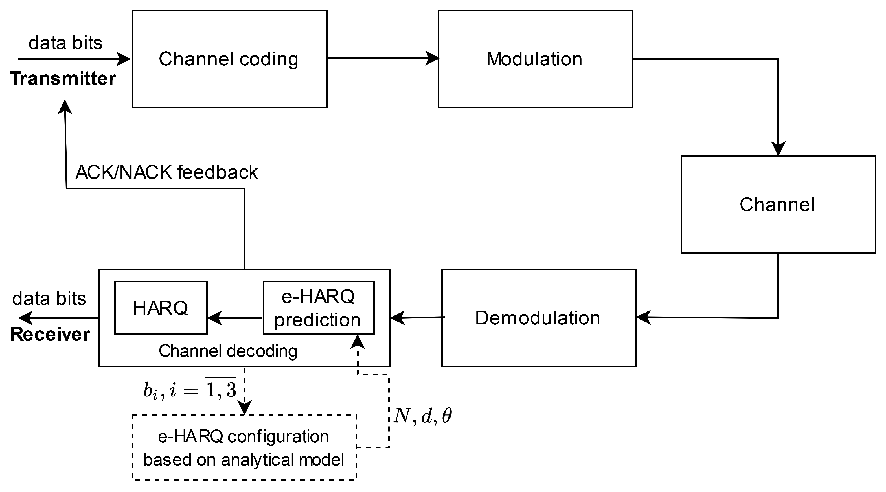
2. System Model
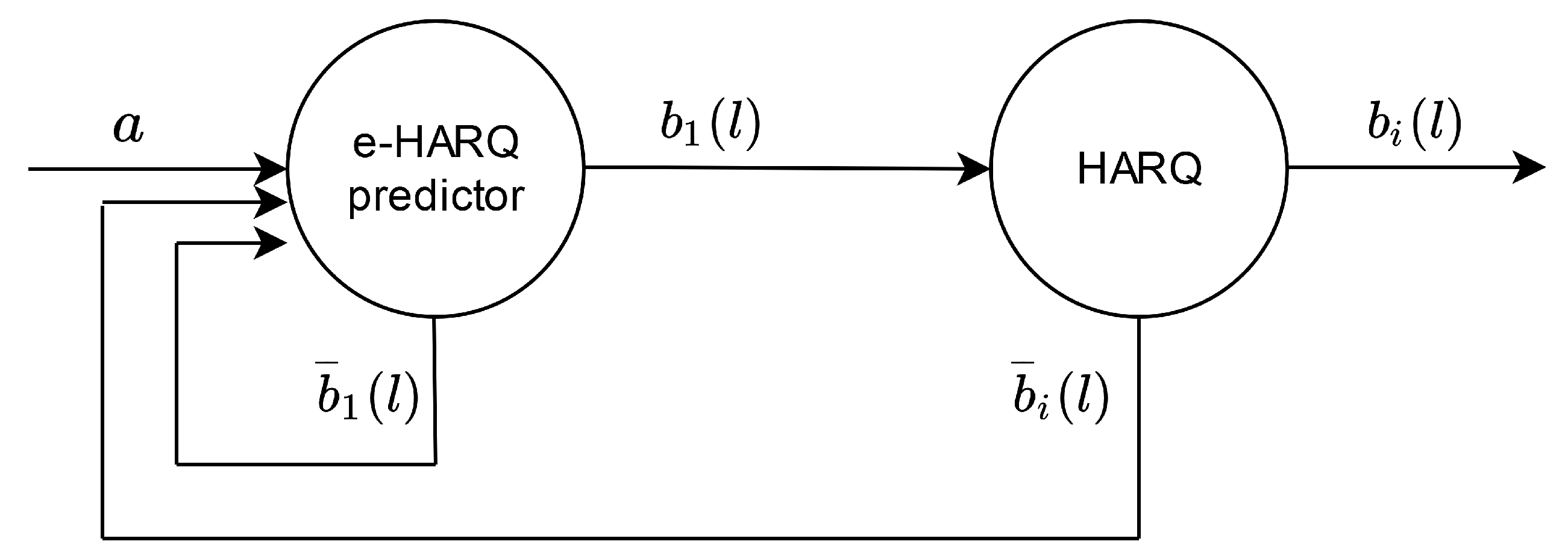
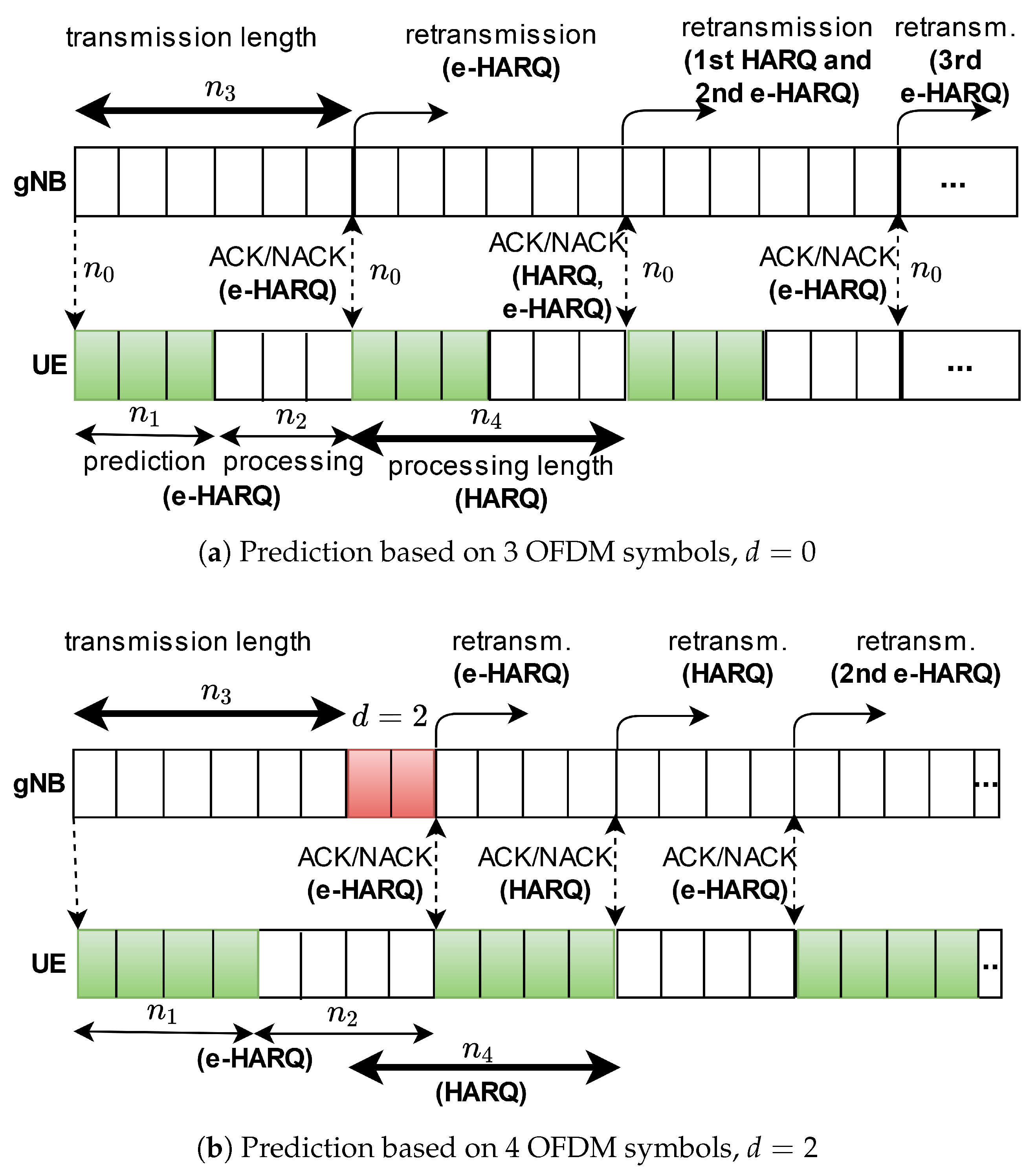
2.1. e-HARQ and HARQ Schemes
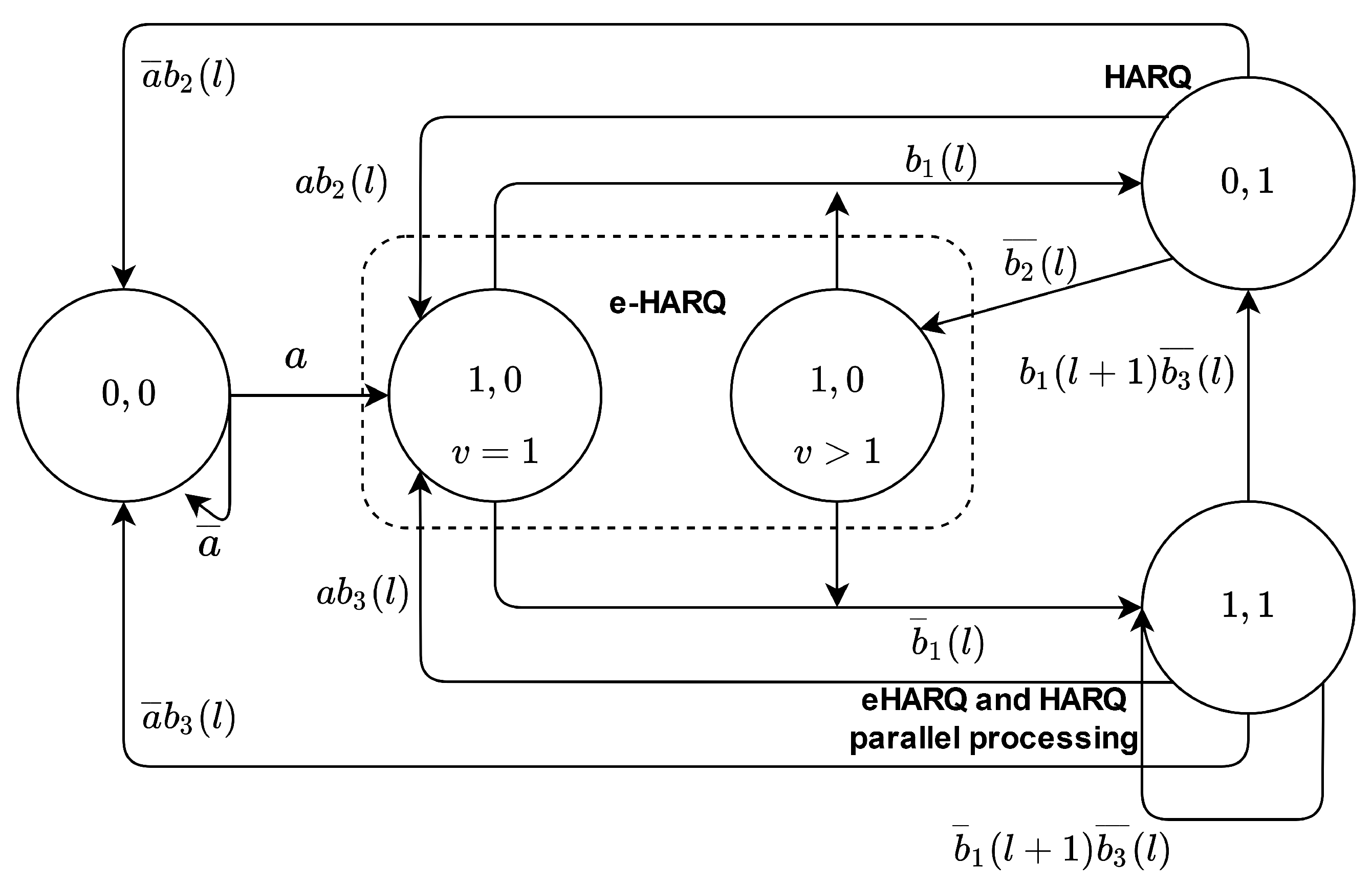
2.2. Model Description
2.3. Balance Equations
2.4. Performance Measures
3. Experimental Analysis
3.1. Link-Level Simulation Setup
3.2. Validation of the Model
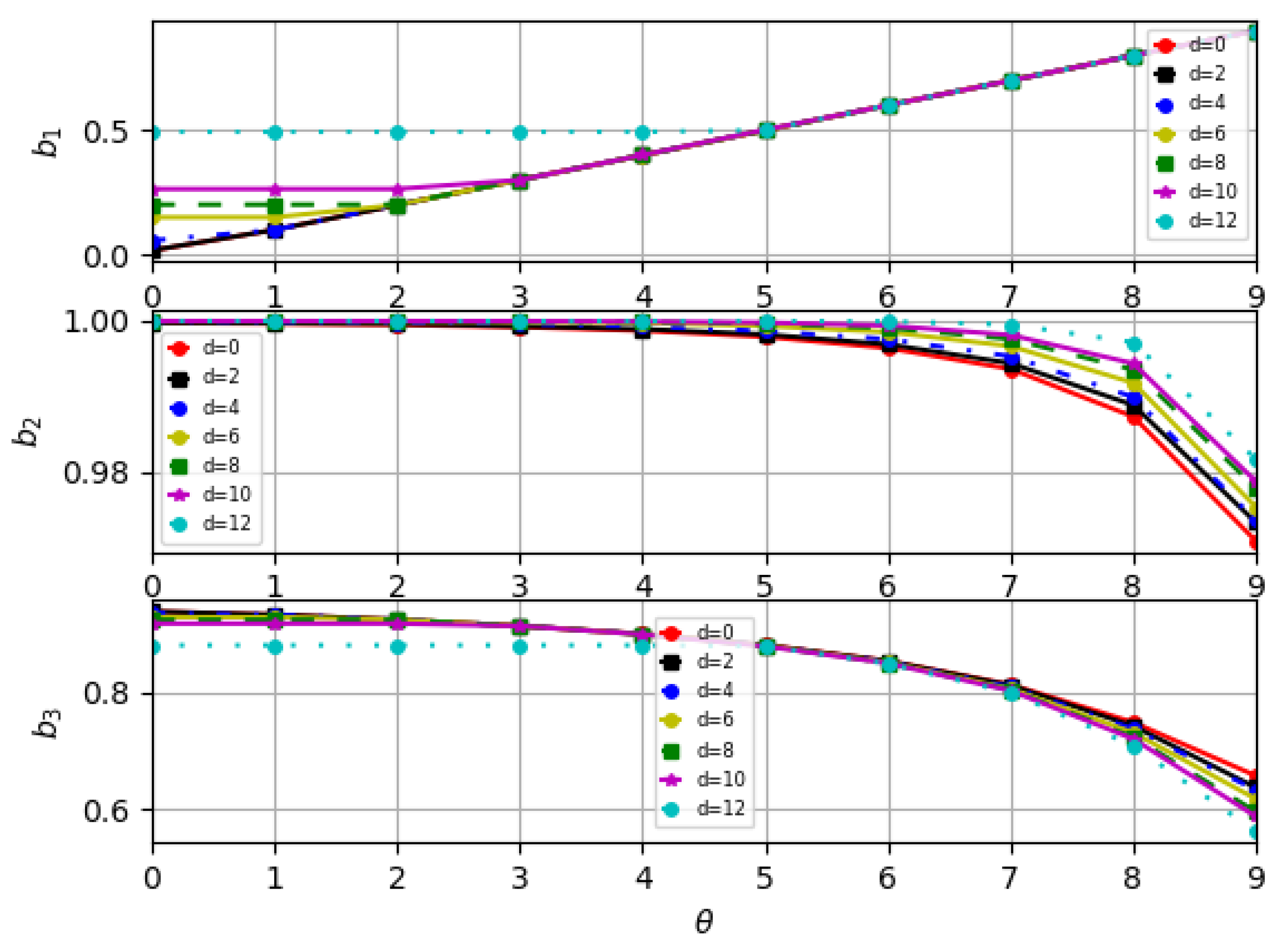
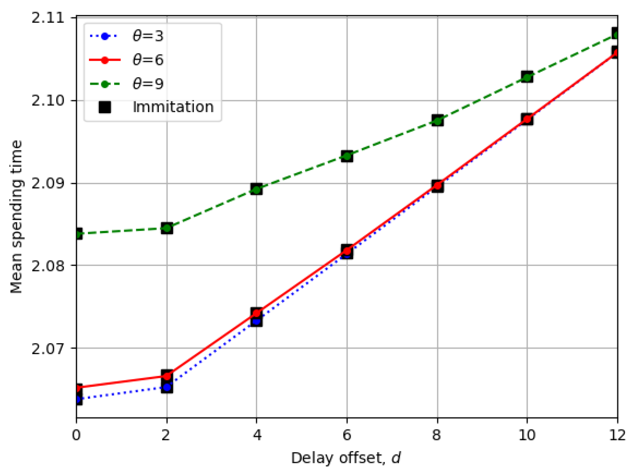
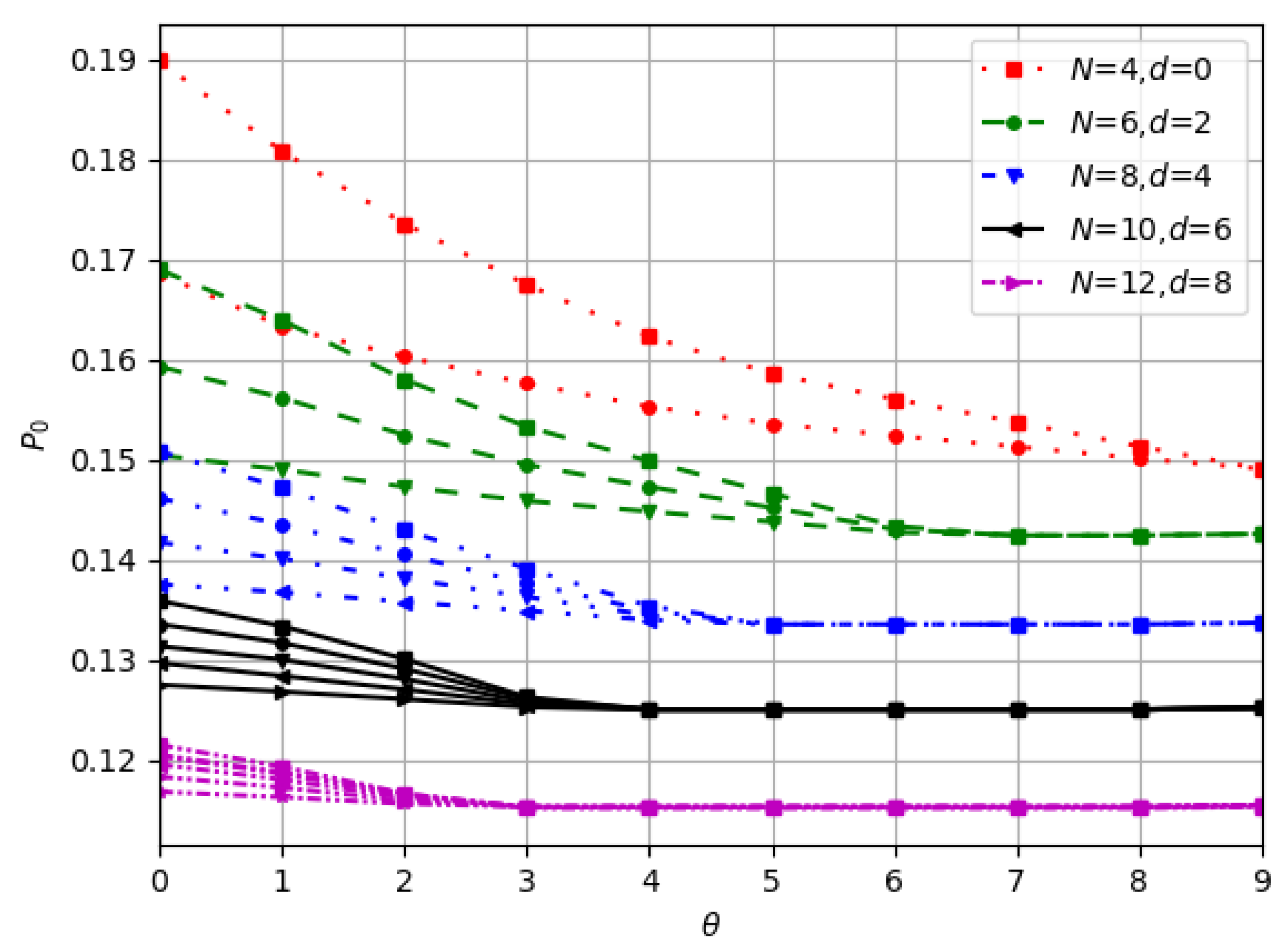
3.3. Analysis of Model’s Tendencies
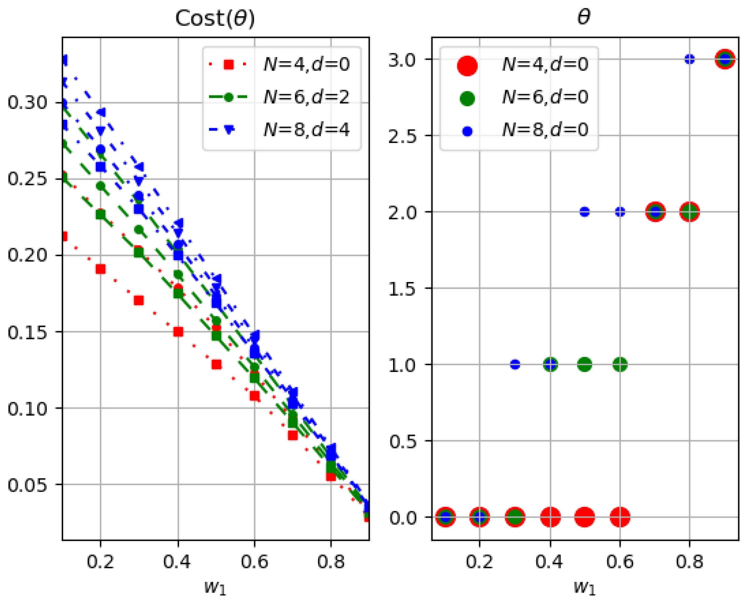
3.4. Optimization Analysis
4. Discussion
Author Contributions
Funding
Acknowledgments
Conflicts of Interest
References
- Tullberg, H.; Popovski, P.; Li, Z.; Uusitalo, M.A.; Hoglund, A.; Bulakci, O.; Fallgren, M.; Monserrat, J.F. The METIS 5G System Concept: Meeting the 5G Requirements. IEEE Commun. Mag. 2016, 54, 132–139. [Google Scholar] [CrossRef]
- Bertenyi, B.; Nagata, S.; Kooropaty, H.; Zhou, X.; Chen, W.; Kim, Y.; Dai, X.; Xu, X. 5G NR Radio Interface. J. ICT Stand. 2018, 6, 31–58. [Google Scholar] [CrossRef]
- 3GPP. 3GPP Release 16. Technical Report. 2020. Available online: https://www.3gpp.org/release-16 (accessed on 20 June 2021).
- Xu, D.; Zhou, A.; Zhang, X.; Wang, G.; Liu, X.; An, C.; Shi, Y.; Liu, L.; Ma, H. Understanding Operational 5G: A First Measurement Study on Its Coverage, Performance and Energy Consumption. In Proceedings of the Annual Conference of the ACM Special Interest Group on Data Communication on the Applications, Technologies, Architectures, and Protocols for Computer Communication, Online, 10–14 August 2020; ACM: New York, NY, USA, 2020; pp. 479–494. [Google Scholar] [CrossRef]
- 3GPP TS 38.211. Physical Channels and Modulation. v15.7.0. Available online: https://www.3gpp.org/ftp//Specs/archive/38_series/38.211/38211-f70.zip (accessed on 20 June 2021).
- 3GPP TS 38.214. Physical Layer Procedures for Data. v15.7.0. Available online: https://www.3gpp.org/ftp//Specs/archive/38_series/38.214/38214-f70.zip (accessed on 20 June 2021).
- Nokia Shanghai Bell. Enhanced Industrial Internet of Things (IoT) and URLLC Support. Technical Report RP-193233, 3GPP. 2019. Available online: https://www.3gpp.org/ftp/TSG_RAN/TSG_RAN/TSGR_86/Docs/RP-193233.zip (accessed on 18 June 2021).
- Frederiksen, F.; Kolding, T.E. Performance and modeling of WCDMA/HSDPA transmission/H-ARQ schemes. In Proceedings of the IEEE 56th Vehicular Technology Conference, Vancouver, BC, Canada, 24–28 September 2002; Volume 1, pp. 472–476. [Google Scholar] [CrossRef]
- Mahmood, N.H.; Abreu, R.; Bohnke, R.; Schubert, M.; Berardinelli, G.; Jacobsen, T.H. Uplink Grant-Free Access Solutions for URLLC services in 5G New Radio. In Proceedings of the 2019 16th International Symposium on Wireless Communication Systems (ISWCS), Oulu, Finland, 27–30 August 2019; pp. 607–612. [Google Scholar] [CrossRef] [Green Version]
- Liu, Y.; Deng, Y.; Elkashlan, M.; Nallanathan, A.; Karagiannidis, G.K. Analyzing Grant-Free Access for URLLC Service. arXiv 2020, arXiv:2002.07842. [Google Scholar] [CrossRef]
- Shariatmadari, H.; Duan, R.; Iraji, S.; Li, Z.; Uusitalo, M.; Jäntti, R. Resource Allocations for Ultra-Reliable Low-Latency Communications. Int. J. Wirel. Inf. Netw. 2017, 24, 317–327. [Google Scholar] [CrossRef]
- Shariatmadari, H.; Duan, R.; Iraji, S.; Jäntti, R.; Li, Z.; Uusitalo, M.A. Asymmetric ACK/NACK Detection for Ultra—Reliable Low—Latency Communications. In Proceedings of the 2018 European Conference on Networks and Communications (EuCNC), Ljubljana, Slovenia, 18–21 June 2018; pp. 1–166. [Google Scholar] [CrossRef] [Green Version]
- Letzepis, N.; Grant, A. Bit Error Estimation for Turbo Decoding. In Proceedings of the IEEE International Symposium on Information Theory, Yokohama, Japan, 29 June–4 July 2003. [Google Scholar] [CrossRef]
- Berardinelli, G.; Khosravirad, S.R.; Pedersen, K.I.; Frederiksen, F.; Mogensen, P. Enabling Early HARQ Feedback in 5G Networks. In Proceedings of the 83rd IEEE Vehicular Technology Conference (VTC Spring), Nanjing, China, 15–18 May 2016; pp. 1–5. [Google Scholar] [CrossRef]
- Berardinelli, G.; Khosravirad, S.R.; Pedersen, K.I.; Frederiksen, F.; Mogensen, P. On the benefits of early HARQ feedback with non-ideal prediction in 5G networks. In Proceedings of the International Symposium on Wireless Communication Systems (ISWCS), Poznan, Poland, 20–23 September 2016; pp. 11–15. [Google Scholar]
- Göktepe, B.; Fähse, S.; Thiele, L.; Schierl, T.; Hellge, C. Subcode-based Early HARQ for 5G. In Proceedings of the IEEE International Conference on Communications (ICC) Workshops, Kansas City, MO, USA, 20–24 May 2018. [Google Scholar] [CrossRef]
- Rykova, T.; Göktepe, B.; Schierl, T.; Hellge, C. Analytical Model of Early HARQ Feedback Prediction. In Internet of Things, Smart Spaces, and Next Generation Networks and Systems; Springer International Publishing: New York, NY, USA, 2020; pp. 222–239. [Google Scholar]
- Makki, B.; Svensson, T.; Caire, G.; Zorzi, M. Fast HARQ Over Finite Blocklength Codes: A Technique for Low-Latency Reliable Communication. IEEE Trans. Wirel. Commun. 2019, 18, 194–209. [Google Scholar] [CrossRef] [Green Version]
- Hou, Z.; She, C.; Li, Y.; Zhuo, L.; Vucetic, B. Prediction and Communication Co-Design for Ultra-Reliable and Low-Latency Communications. IEEE Trans. Wirel. Commun. 2020, 19, 1196–1209. [Google Scholar] [CrossRef]
- Ericsson. Way Forward on Processing Timing Reduction for sTTI. Technical Report R1-165854; 3GPP. 2016. Available online: https://www.3gpp.org/ftp/TSG_RAN/WG1_RL1/TSGR1_85/Docs/R1-165854.zip (accessed on 18 June 2021).
- Hastie, T.; Tibshirani, R.; Friedman, J. The Elements of Statistical Learning; Springer Series in Statistics; Springer: New York, NY, USA, 2001. [Google Scholar]
- MCC Support. 3GPP TS 38.212 v16.0.0. Technical Report, 3GPP. 2020, pp. 19–30. Available online: https://www.3gpp.org/ftp//Specs/archive/38_series/38.212/38212-g00.zip (accessed on 20 June 2021).
- Strodthoff, N.; Göktepe, B.; Schierl, T.; Hellge, C.; Samek, W. Enhanced Machine Learning Techniques for Early HARQ Feedback Prediction in 5G. IEEE J. Sel. Areas Commun. 2019, 37, 2573–2587. [Google Scholar] [CrossRef] [Green Version]


| s | Description | States Path |
|---|---|---|
| 0 | Empty system | |
| (0,0) | ||
| 1 | The partial codeword is being processed at phase 1 | 0() |
| (1,0) | ||
| 2 | The packet is processed at phase 2 due to ACK at phase 1 | 2(), |
| (0,1) | 4() | |
| 3 | The packet is being retransm. At phase 1 because of NACK, and previous negatively acknowledged packet is being processed at phase 2 | 3() |
| (1,1) | 5() |
| Transport block size () | 500 |
| Transmission bandwidth | 1.08 MHz (6 RBs) |
| Channel Code | Rate-1/5 LDPC [22] |
| Modulation order and algorithm | 64-QAM, Approx. LLR |
| Power allocation | Constant |
| Waveform | 3GPP OFDM, normal cyclic-prefix, 15 kHz spacing |
| Channel type | 1 Tx 1 Rx, TDL-C 100 ns, 7 GHz, 3 km/h |
| Equalizer | Freq. domain MMSE |
| SNR | 5.0 dB:12.0 dB |
| Decoder type | Min-Sum (50 iter.) |
| Predictor type | Logistic regressions [23] (5 iter.) |
| SNR | ||||||||||||
|---|---|---|---|---|---|---|---|---|---|---|---|---|
| 5 | 1.32 | 4.41 | 5.23 | 6.17 | 1.60 | 5.62 | 8.17 | 40.80 | 2.48 | 9.52 | 28.51 | 40.80 |
| 6 | 1.12 | 2.51 | 5.68 | 6.86 | 1.97 | 3.58 | 7.8 | 39.6 | 3.23 | 9.3 | 26.3 | 39.67 |
| 7 | 1.27 | 3.12 | 5.72 | 6.76 | 1.98 | 4.65 | 15.04 | 39.09 | 4.75 | 9.89 | 23.48 | 39.09 |
| 8 | 0.65 | 2.43 | 4.62 | 5.81 | 2.45 | 5.2 | 21.58 | 37.43 | 5.77 | 8.41 | 26.43 | 37.43 |
| 9 | 0.55 | 1.67 | 3.38 | 6.02 | 2.87 | 8.78 | 18.07 | 32.33 | 6.4 | 18.70 | 23.70 | 32.33 |
| 10 | 0.3 | 1.47 | 2.87 | 2.87 | 3.3 | 7.51 | 21.3 | 27.37 | 12.36 | 16.46 | 21.3 | 27.37 |
| 11 | 0.71 | 1.42 | 2.08 | 9.85 | 4.73 | 8.10 | 18.14 | 22.78 | 9.84 | 13.63 | 18.14 | 22.78 |
| 12 | 0.68 | 2.29 | 7.62 | 7.62 | 5.32 | 7.15 | 15.51 | 19.53 | 8.35 | 11.40 | 15.51 | 19.53 |
Publisher’s Note: MDPI stays neutral with regard to jurisdictional claims in published maps and institutional affiliations. |
© 2021 by the authors. Licensee MDPI, Basel, Switzerland. This article is an open access article distributed under the terms and conditions of the Creative Commons Attribution (CC BY) license (https://creativecommons.org/licenses/by/4.0/).
Share and Cite
Rykova, T.; Göktepe, B.; Schierl, T.; Samouylov, K.; Hellge, C. Analytical Model and Feedback Predictor Optimization for Combined Early-HARQ and HARQ. Mathematics 2021, 9, 2104. https://doi.org/10.3390/math9172104
Rykova T, Göktepe B, Schierl T, Samouylov K, Hellge C. Analytical Model and Feedback Predictor Optimization for Combined Early-HARQ and HARQ. Mathematics. 2021; 9(17):2104. https://doi.org/10.3390/math9172104
Chicago/Turabian StyleRykova, Tatiana, Barış Göktepe, Thomas Schierl, Konstantin Samouylov, and Cornelius Hellge. 2021. "Analytical Model and Feedback Predictor Optimization for Combined Early-HARQ and HARQ" Mathematics 9, no. 17: 2104. https://doi.org/10.3390/math9172104
APA StyleRykova, T., Göktepe, B., Schierl, T., Samouylov, K., & Hellge, C. (2021). Analytical Model and Feedback Predictor Optimization for Combined Early-HARQ and HARQ. Mathematics, 9(17), 2104. https://doi.org/10.3390/math9172104