Article

On the Classification of MR Images Using “ELM-SSA” Coated Hybrid Model

1
Department of Computer Science and Engineering, Siksha ‘O’ Anusandhan Deemed to Be University, Bhubaneswar 751030, Odisha, India
2
Department of Electronics and Tele Communication, C. V. Raman Global University, Bhubaneswar 752054, Odisha, India
3
College of Information Business Systems, National University of Science and Technology, MISIS, Leninsky Prospect 4, 119049 Moscow, Russia
4
Department of Computer Science, South Ural State University, 454080 Chelyabinsk, Russia
*
Authors to whom correspondence should be addressed.
Mathematics 2021, 9(17), 2095; https://doi.org/10.3390/math9172095
Submission received: 15 July 2021 / Revised: 24 August 2021 / Accepted: 26 August 2021 / Published: 30 August 2021
(This article belongs to the Special Issue Intelligent Computing in Industry Applications)

Abstract

:
Computer-aided diagnosis permits biopsy specimen analysis by creating quantitative images of brain diseases which enable the pathologists to examine the data properly. It has been observed from other image classification algorithms that the Extreme Learning Machine (ELM) demonstrates superior performance in terms of computational efforts. In this study, to classify the brain Magnetic Resonance Images as either normal or diseased, a hybridized Salp Swarm Algorithm-based ELM (ELM-SSA) is proposed. The SSA is employed to optimize the parameters associated with ELM model, whereas the Discrete Wavelet Transformation and Principal Component Analysis have been used for the feature extraction and reduction, respectively. The performance of the proposed “ELM-SSA” is evaluated through simulation study and compared with the standard classifiers such as Back-Propagation Neural Network, Functional Link Artificial Neural Network, and Radial Basis Function Network. All experimental validations have been carried out using two different brain disease datasets: Alzheimer’s and Hemorrhage. The simulation results demonstrate that the “ELM-SSA” is potentially superior to other hybrid methods in terms of ROC, AUC, and accuracy. To achieve better performance, reduce randomness, and overfitting, each algorithm has been run multiple times and a k-fold stratified cross-validation strategy has been used.

1. Introduction

To facilitate doctors for diagnosis of brain disease, proper analysis and classification of various types of brain images are required. The conventional images used for this purpose are Computed Tomography, Positron Emanation Tomography, Ultrasonography, X-radiation, and Magnetic Resonance Imaging (MRI). Out of these techniques, the MRI serves as a better source of information for brain study and it helps to recognize tissues with a higher spatial resolution. However, its analysis is complex and time-consuming. Consequently, a computerized framework needs to be developed for automatic diagnosis using appropriate Computer-Aided Diagnosis (CAD) arrangement.
The MRI is a useful asset for imaging of the human cerebrum which uses radiology waves and magnetic fields. For biomedical research and clinical examination, it provides adequate data of the delicate mind tissues [1]. The MRI gives a better quality contrast for various cerebrum tissues and creates fewer antiquities [2,3,4] compared to other imaging processes. The CAD-based analysis from MR pictures has gained increasing importance among researchers [5]. For appropriate classification of MR pictures, the extracted features play an important role.
The Extreme Learning Machine (ELM) is chosen for the classification of brain images as it processes faster. In ELM architecture, the weights and biases are initialized randomly, and the proper weights of the model are obtained using Moore–Penrose (MP) generalized inverse. The ELM model has proven to be useful and reliable classifier for many applications [6]. To further improve the performance of the ELM network, its associated conventional weights have been optimized using bioinspired Salp Swarm Algorithm (SSA) [7]. The major challenge lies is extraction of required features from MR images and subsequent reduction of less important features which assist in reducing the classification complexity.
To achieve better final weights of various Artificial Neural Network (ANN) structures during the training phase, different evolutionary computing techniques have been employed [8,9,10]. The single hidden layer feedforward hidden layer network is a standard ANN structure that trained by the back-propagation (BP) learning utilizing gradient descent strategy which minimizes the cost function. However, BP-based learning is sensitive to initial weights and convergence rate is slower. To improve the learning rate, momentum and step size variation have been introduced [11,12,13,14]. The ELM is a faster model proposed by Huang et al. [15], which used arbitrary initial weights and biases, and final weights are obtained using MP generalized inverse.
In a recent work [3], the Support Vector Machine (SVM) classifier employs Two-Dimensional Discrete Wavelet Transformation (2D-DWT)-based features of MR image and is reported to provide 4% more accuracy than the Self-Organizing Map model. In another study, El-Dahshan et al. [16] have used 2D-DWT and PCA for feature extraction and reduction, and K-Nearest Neighbor (KNN) and Back-Propagation Neural Network (BPNN) for classification of MR images. From the simulation study, it is observed that the average performance of KNN is superior to the BPNN. To improve the accuracy, swarm intelligence techniques are used to tune the model parameters [17,18]. The authors of [19,20] have suggested an ELM training using Differential Evolution (DE) and Particle Swarm Optimization (PSO) optimization. For classification task, the BPNN model have used different filters for preprocessing the images and Feedback Pulse Coupled Neural Network has been used for segmentation technique, and both 2D-DWT and PCA for extraction and reduction of features respectively [21]. Dehuri, S. et al. [22] have proposed an improved particle swarm optimization technique to train Functional Link Artificial Neural Network (FLANN) architecture for classification of brain tumor MRI images as malignant or benign. As the FLANN is a single-layered structure, it requires fewer parameters to be tuned. In this article, the authors have optimized FLANN weights and have achieved good classification accuracy as compared to FLANN with gradient descent learning and SVM model with radial basis function kernel. In another communication, Chao Ma. et al. [23] have applied the Artificial Bee Colony optimization technique to adjust the parameters of the ELM architecture and obtained a better generalization performance in terms of classification accuracy. Eusuff et al. [24] have suggested a Shuffled Frog Leaping Algorithm approach to tune ELM parameters [25]. The authors of [26] have employed the Salp Swarm Algorithm (SSA) [27] in SVM + RBF hybridized model for classification of MR images. They have reported an accuracy of 0.9833, sensitivity of 1, and specificity of 0.9818 which are better than those obtained from SVM classifier.
Different variations of 2D-DWT have been used for feature extraction in classification task, however for obtaining higher accuracy, the authors have used a smaller dataset. The motivation and objective of this work is as follows:
(i)
To develop an automatic biomedical image classification model offering satisfactory and reliable performance using large MR image datasets.
(ii)
To further improve the performance, hybridized models are proposed for tuning the parameters of the models using bioinspired optimization techniques.
(iii)
The lack of salp inspired algorithms in literature is a main motivation of this paper.
In this study, the classification task is carried out using ELM [28,29,30], FLANN, RBFN, and BPNN machine learning models. The SSA, PSO, and DE optimization methods have been utilized for achieving best possible parameters of the models. The main contributions of this paper are listed below.
(i)
Which activation function of ELM network has yielded faster convergence during training?
(ii)
Which bioinspired technique optimized the ELM parameters in a better way?
(iii)
How much performance improvement was achieved using proper classification models?
(iv)
ELM-SSA exhibits superior performance over FLANN, RBFN, and BPNN models hybridized with PSO, DE as well as SSA schemes.
(v)
On average, the ELM-SSA model yields lower execution time compared to other models.
(vi)
In general, the proposed ELM-SSA model outperforms other hybridized classification models such as FLANN-SSA with an improvement in accuracy of 5.31% and 1.02% for Alzheimer’s and Hemorrhage datasets, respectively.
(vii)
The ELM-SSA model has produced 8.79% and 2.06% better accuracy as compared to RBFN-SSA for two datasets.
(viii)
ELM-SSA has also shown 7.6% and 1.02% higher accuracy for the two datasets, respectively, as compared to BPNN-SSA.
The proposed ELM-SSA utilizes the Contrast-Limited Adaptive Histogram Equalization (CLAHE) [31,32] for preprocessing purpose, in addition, the 2D-DWT and PCA are chosen for extraction and reduction of features respectively. A 5 × 5 fold stratified cross-validation scheme is used to preserve the imbalanced class distribution. From the simulation of different datasets, it is observed that the proposed approach demonstrates better accuracy in contrast to other hybridized classifiers.
The rest of the article is organized as follows. Section 2 describe with different methodologies adopted in this work. Concise presentation of various sub-block of the hybrid model is presented in Section 3. Section 4 provides the detail simulation based experiment of the model and finally in Section 5, the conclusion and findings of this work are summarized.

2. Materials and Methods

This section provides a detailed description of the data set and the methodologies adopted in this study. The methodology comprises of five substages: (1) level-3 2D-DWT for extraction of features, (2) feature reduction employ using PCA, (3) overfitting control using stratified k-fold cross-validation, (4) development of ELM classifier, and (5) use of SSA to adjust the parameters of ELM.

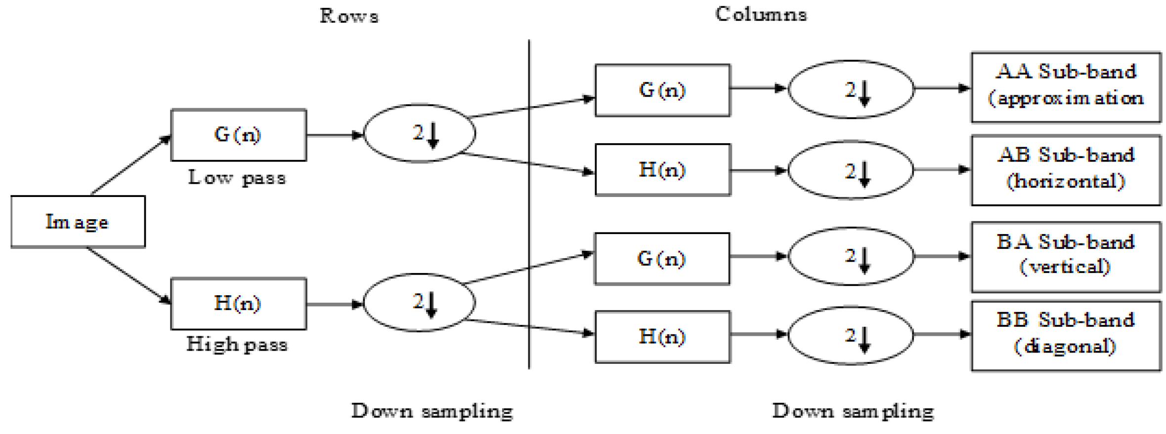
2.1. 2D-DWT for Feature Extraction

The CLAHE [32] preprocessing method based on histogram equalization is used to retain the sharpness of the images and to enhance the edges, the Wavelet Transform (WT) has the potentiality to retain time frequency information and thus is better suited for extracting the features.
The WT of a continuous function like f ( x ) , related to a wavelet function φ ( x ) is described using Equations (1) and (2).
W φ ( s , t ) = + f ( x ) φ s , t ( x ) d x
φ s , t ( x ) = 1 s φ x s t ; s R + , t R +
φ s , t ( x ) is built from the parent wavelet φ ( x ) by utilizing the dilation factor S and translation parameter t. Preventing the parameters s and t with s = 2 J and t = 2 j k . The discrete version of Equation (1) has been mentioned in Equation (3).
D W T f ( n ) = P j , k ( n ) = n f ( n ) G j × n 2 j k Q j , k ( n ) = n f ( n ) H j × n 2 j k
where P j , k ( n ) and Q j , k ( n ) refer to the approximate and detail components, respectively. The parameters j and k represent wavelet scale and translation factors, respectively. The functions G ( n ) and H n represent the low-pass and high-pass filters, respectively. It combines these High-Pass and Low-Pass filters and then downsamplers (DS) by a factor of two. The filter bank approach DWT when applied to MR image, the sub-bands obtained after two stages is shown in Figure 1. Four different sub-bands are AA for (LOW–LOW), AB for (LOW–HIGH), BA for (HIGH–LOW), and BB for (HIGH–HIGH), and they are obtained as shown in Figure 1.
As the Haar wavelet is symmetric and performs better with noisy data, it is chosen in this case. The wavelet coefficients are arranged as a feature vector (FV). If there are M images and N features per image, a Feature Matrix (FM) of size M × N is generated. Algorithm 1 represents the steps required to obtain the FM.
Algorithm 1 Extraction of Feature Matrix (FM)
Input: M: Total number of pictures having size C × C .
Output: FM having size [ 1 : M , 1 : N ] : The coefficients of the L-3 Haar wavelet is calculated by w a v e A p p C o e f f ( ) .
Step 1: Initialize, i = 1 , N C 8 × C 8 (Amount of extracted features)
Step 2: Generate an empty matrix E M [ 1 : C 8 , 1 : C 8 ] and empty vector E V [ 1 , 1 : N ]
Step 3: for n = 1 to M do
Step 4: Obtain M R I n n th MR image
Step 5: E M n 1 : C 8 , C 8 w a v e A p p C o e f f ( )
Step 6: while i N do
Step 7: for s = 1 C 8 do
Step 8: for t = 1 C 8 do
Step 9: F V n [ 1 , i ] E M n [ s , t ]
Step 10: i = i + 1
Step 11: end for
Step 12: end for
Step 13: end while
Step 14: F M [ n , ( 1 : N ) ] F V n [ 1 , ( 1 : N ) ]
Step 15: end for
Before reducing the features by the PCA, the FM needs to be normalized by Z-score normalization which is calculated by subtracting the mean from observed feature value and then dividing the standard deviation

2.2. Principal Component Analysis (PCA) for Reducing Features

Independent component analysis (ICA) and PCA are well-known methods for transforming the higher dimension feature vector into a lower dimension FV [33]. In contrast to ICA, PCA involves less computational complexity and very less complexity also, so most researchers widely used this methodology. The algorithmic steps of PCA are explained in Algorithm 2.
Algorithm 2 Feature reduction using PCA [34]
Input: Primary feature vector.
Output: Reduced feature vector. Let X be an input data set of N points and each having p dimensions, which is represented by Equation (4) .
X = X 1 , 1 X 1 , p X N , 1 X N , p

Step1: Compute the mean of X ( X ¯ : ) which is represented by Equation (5)
X ¯ = 1 N i = 1 N X i

Step 2: Find out the deviation from mean: Q = X X ¯
Step 3: Calculate the covariance matrix C Q which is mentioned in Equation (6)
C Q = i = 1 N X i X i ¯ T × X i X i ¯ N 1
where the correlation between these two dimensions such as i and j are represented by Equation (7):
C Q ( i , j ) = C Q ( j , i ) = k = 1 N ( Q ( k , i ) × Q ( k , j ) ) N 1

If C Q ( i , j ) > 0 , then both ( i , j ) are similar. if C Q ( i , j ) = 0 , then both ( i , j ) are independent. if C Q ( i , j ) 0 , then i and j are opposite.
Step 4: Compute the Eigen Vectors and Eigen Values of C Q .
Step 5: Rearrange the Eigen Vectors and Eigen Values: λ 1 22 . λ n
Step 6: The Eigenvectors having the biggest Eigenvalues come to a new space which consists of the essential coefficients, is represented through Equation (8).
Feature Vector = e g 1 , e g 2 , , e g n

2.3. k-Fold Cross-Validation

During the training of the classifier, the overfitting problem may occur by generating less error value but while testing with new data, the error produced is high. Therefore, to avoid such overfitting problem k-fold cross-validation scheme is used. In this scheme, the whole dataset is divided randomly into a k-fold partition where one fold is required for testing and the remaining folds are used for training. Finally, the mean of the error generated in all sets are calculated. This process is repeated until each fold data is tested.

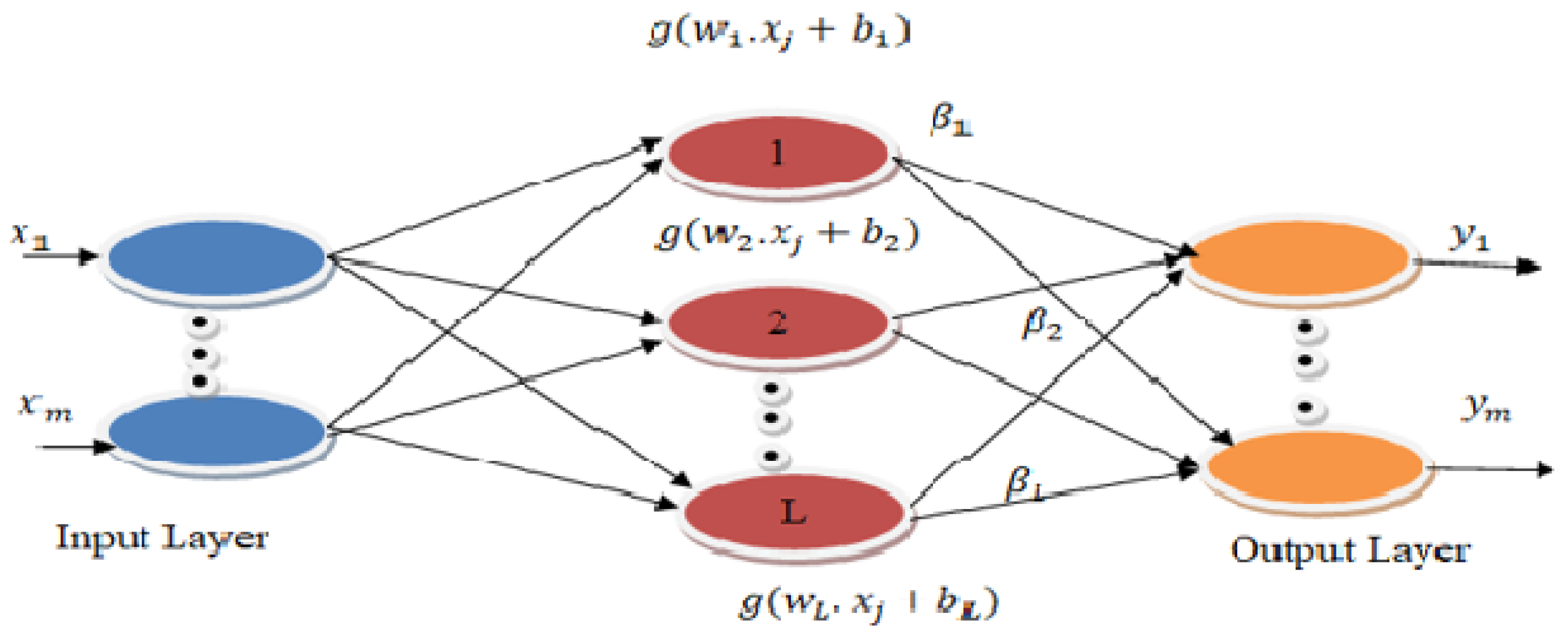
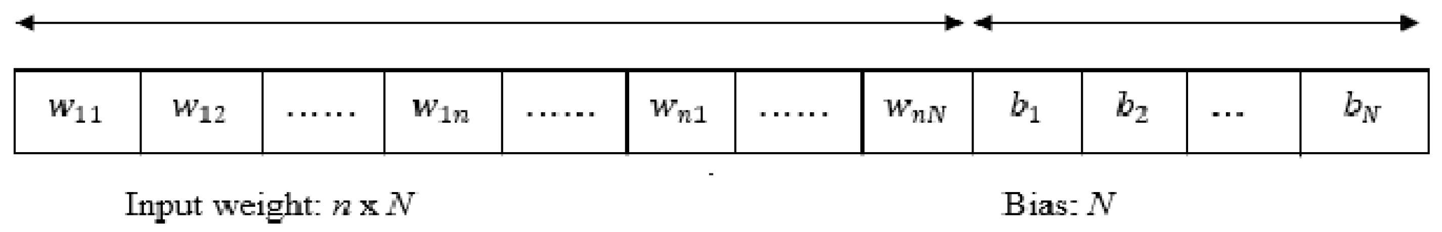
2.4. Classification Using ELM

The ELM-SSA classifier is employed in the brain MR images for binary classification. The ELM is one of the best learning frameworks which was proposed by Huang in 2006 [15]. It has a good generalization performance along with a faster learning rate as compared to traditional learning techniques such as the SVM, Back-Propagation, ANN, Least Square-SVM, etc. It contains only one hidden layer of which the weights and bias values are adjusted. Instead of gradient descent based back propagation learning, it uses MP generalized inverse technique to find output weights. Figure 2 represents the schematic diagram of the ELM model.
The expression of actual output of the above schematic structure is represented by Equation (9).
O j = i = 1 L β i g w i · x j + b i , i = 1 , 2 , L , j = 1 , 2 , m
where x and y are input and output vectors, respectively; b i is a bias of i t h hidden neurons; the weight vector between input and hidden layer is represented by w i = [ w i 1 , w i 2 ] ; and m and L denote the number of the training sample and hidden nodes, respectively. O j represents the output vector of the jth input vector. The output weight matrix ( β ) joins ith hidden nodes with output neurons and g ( x ) is an activation function.
The ELM starts with arbitrary m distinct samples with zero error, which is represented through Equation (10).
j = 1 m O j y j = 0
Given a training set as ( x j , y j ) , here x j = x i 1 , x i 2 , x i N T , y j = y 1 , y 2 , y Q T , where Q and N are target values and number of variables, respectively. The relationship between Hidden layer output matrix ( H ) , output weight ( β ) , and target training matrix ( Y ) is expressed by Equation (11). The target training matrix ( Y ) and output weight ( β ) matrix is represented by Equation (12).
H × β = Y
β = β 1 T β 2 T β L T L × Q , Y = Y 1 T Y 2 T Y m T m × Q
H w 1 , , w m , b 1 , , b L , x 1 , x m = g w 1 · x 1 + b 1 g w m · x 1 + b L g w 1 · x m + b 1 g w m · x m + b L m × L
where Equation (13) represents the hidden layer output matrix H and β can be calculated using MP generalized inverse of H which is represented by Equation (14).
β = H + T
where H + denotes MP generalized inverse of H.
As the input weights and biases of ELM are randomly selected, two issues may arise: (i) During the testing phase, it responds slowly, and (ii) in the presence of maximum hidden neurons, it produces a poor generalization performance. Therefore, nature and bioinspired learning strategies are better candidates to tackle these issues. Thus, SSA is chosen for optimizing the weights and bias values of the ELM model.

2.5. Salp Swarm Algorithm (SSA)

Recently, Mirjalili et al. [7] have proposed the SSA in 2017 which is based on the swarming behavior of salps in the ocean. The position vectors of salps are considered as the weights and bias vector. Each salp updates its position vector including leader and followers.
Let X represents salp population dimension of N × d , where N denotes the number of salps with d-dimensions. It is expressed as a matrix, which is shown in Equation (15).
X i = x 1 1 x 1 d x N 1 x N d N × d
The leader’s position ( X j 1 ) is calculated as
X j 1 = F j + C 1 U j L j C 2 + l b j , C 3 0.5 F j C 1 U j L j C 2 + l b j , C 3 < 0.5
where
  • F j : position vector of food source in j t h dimension.
  • U and L: superior and inferior limit, respectively.
  • C 2 , C 3 : are random numbers between 0 and 1.
C 1 is expressed as
C 1 = 2 . e 4 M M 2
where M is the highest value of iterations and C 1 value decreases as iteration count increases. Thus, it figures out how to put more underscore on the expansion tendency in the beginning stages. The locations of followers are updated as
x j i = x j i + x j i 1 2 where ( i 2 )
where X j i represents the position of ith follower at jth direction. Algorithm 3 represents the pseudocode of SSA.
Algorithm 3 Salp Swarm Algorithm pseudocode
Set the population of salp and their upper and lower bound
While (not equal terminate condition) do
Calculate the RMSE for every salp
Consider Leader ( F ) salp having lowest RMSE
Randomly initialize C 2 and C 3 between [0, 1]
Update C 1 by Equation (17)
For (each salp ( x i ) ) do
if ( i = = 1 ) then
Leader salp location updated by Equation (16)
else
Follower salp location updated by Equation (18)
Use upper and lower limit of variables to update the population
Return F
end for loop
end while loop

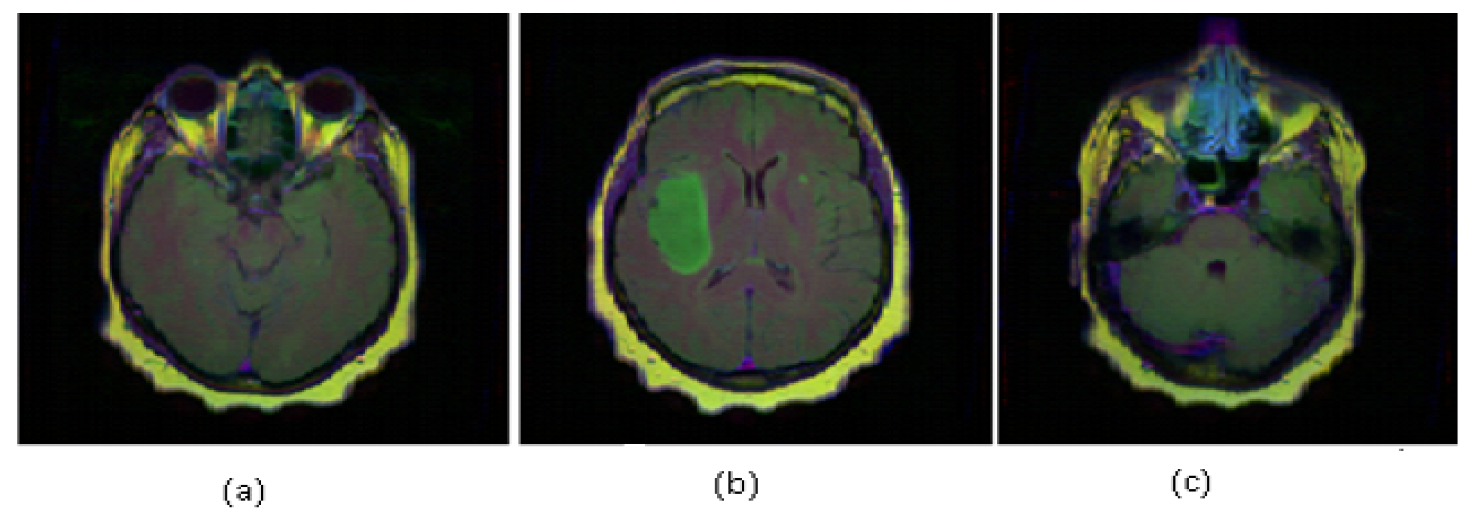
2.6. Data Set Description

In this study, two standard MR image datasets, i.e., Alzheimer’s and Hemorrhage, having 100 and 200 images, respectively, have been used. Each image on the two data sets has a resolution of 256 × 256 . The Kaggle website is the source of images which are of two categories, i.e., normal brain images and abnormal brain images. Table 1 provides the details of the datasets. Each of the dataset contains 1296 number of features and two class labels.
In this article, a 5 × 5 -fold stratified cross-validation technique has been used. Table 2 represents the ratio of number of training and testing images used in Alzheimer’s and Hemorrhage datasets. Therefore, 5 trials have been taken in two datasets from which 80 images (40 for normal images and another 40 for abnormal images) are used in the training phase and the remaining 20 images (10 for normal images and another 10 for abnormal images) are utilized for testing in Alzheimer’s dataset similarly 160 images (80 for normal images and another 80 for abnormal images) have been used in training and remaining 40 images (20 for normal images and another 20 for abnormal images) are employed for testing in Hemorrhage dataset. Each category of brain MR image sample such as normal brain MR image, Alzheimer’s brain MRI, and Hemorrhage brain MRI are represented in Figure 3a–c, respectively .
In this study, a comparative performance has been carried out between the proposed hybrid model, i.e., ELM-based SSA (ELM-SSA) with other existing models such as BPNN, FLANN, and RBFN with other optimization algorithms such as PSO and DE. The performance indices used are accuracy, ROC (Receiver Operating Characteristic Curve), and AUC (Area Under the ROC Curve).

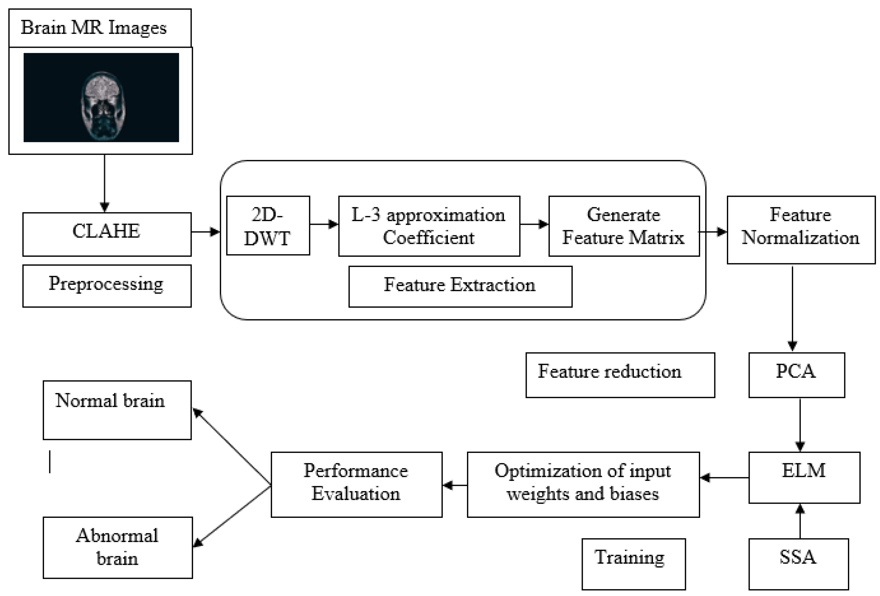
3. Proposed Methodology

The overall scheme of the proposed hybrid technique (ELM-SSA) for the classification of brain MRI is shown in Figure 4.
The methodology SSA based ELM classifier is deal in this section. Each salp of SSA denotes a candidate in the ELM model. Each salp consists of weights and biases of the ELM network where n × N + N represents the salp length. Figure 5 denotes the structure vector of a salp of SSA [35].
In this work, SSA is employed for minimization of misclassification rate which is considered as cost function defined in Equation (19).
f = min ( 1 A c c u r a c y )
Here, A c c u r a c y is computed as
A c c u r a c y = i = 1 n j = 1 c f ( i , j ) c ( i , j ) n
where c represents the total number of classes and n denotes the total number of instances.
f i , j = 1 , if an instance i is of class j else 0.
c i , j = 1 , if the predicted class of instance i is j else 0.

4. Experimental Results and Discussion

This section discusses the experimentation details of the proposed model along with systems configuration, datasets used, parameters setting, validation strategies, and result analysis.

4.1. System Configuration

The simulation-based experiments of the proposed classification model are carried out in this section. The configuration of the computing system used is presented in Table 3.
An Intel(R) Core(TM) i3-6006U with 2 GHz frequency, 8 GB main memory, Windows 7 operating system and the statistical toolbox of Mat lab R2015a platform have been used for our experiment.

4.2. Performance Evaluation

The various performance measures used are given below.
  • Accuracy: It finds how many brain images are classified correctly from the total image sets tested.
    A c c u r a c y = t p e + t n e t p e + t n e + f p e + f n e
    where t p e = True Positive, t n e = True Negative, f p e = False Positive, f n e = False Negative.
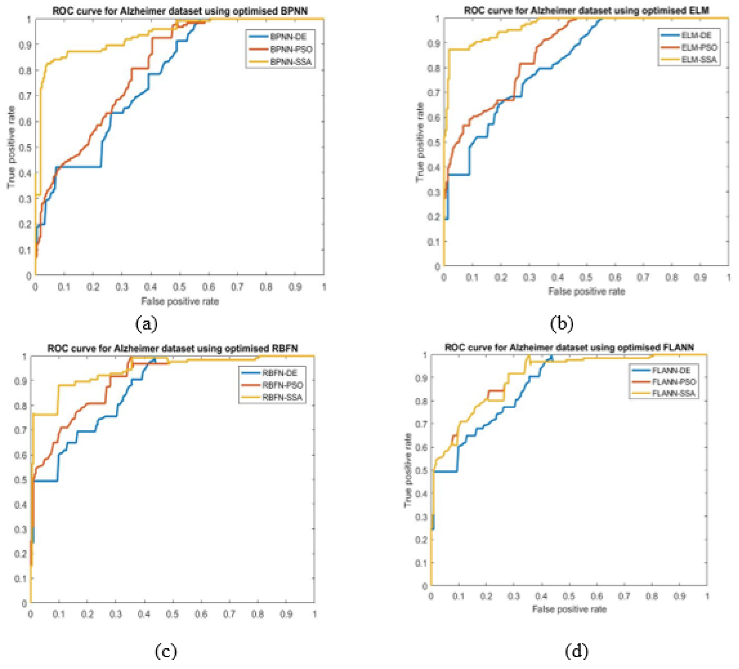
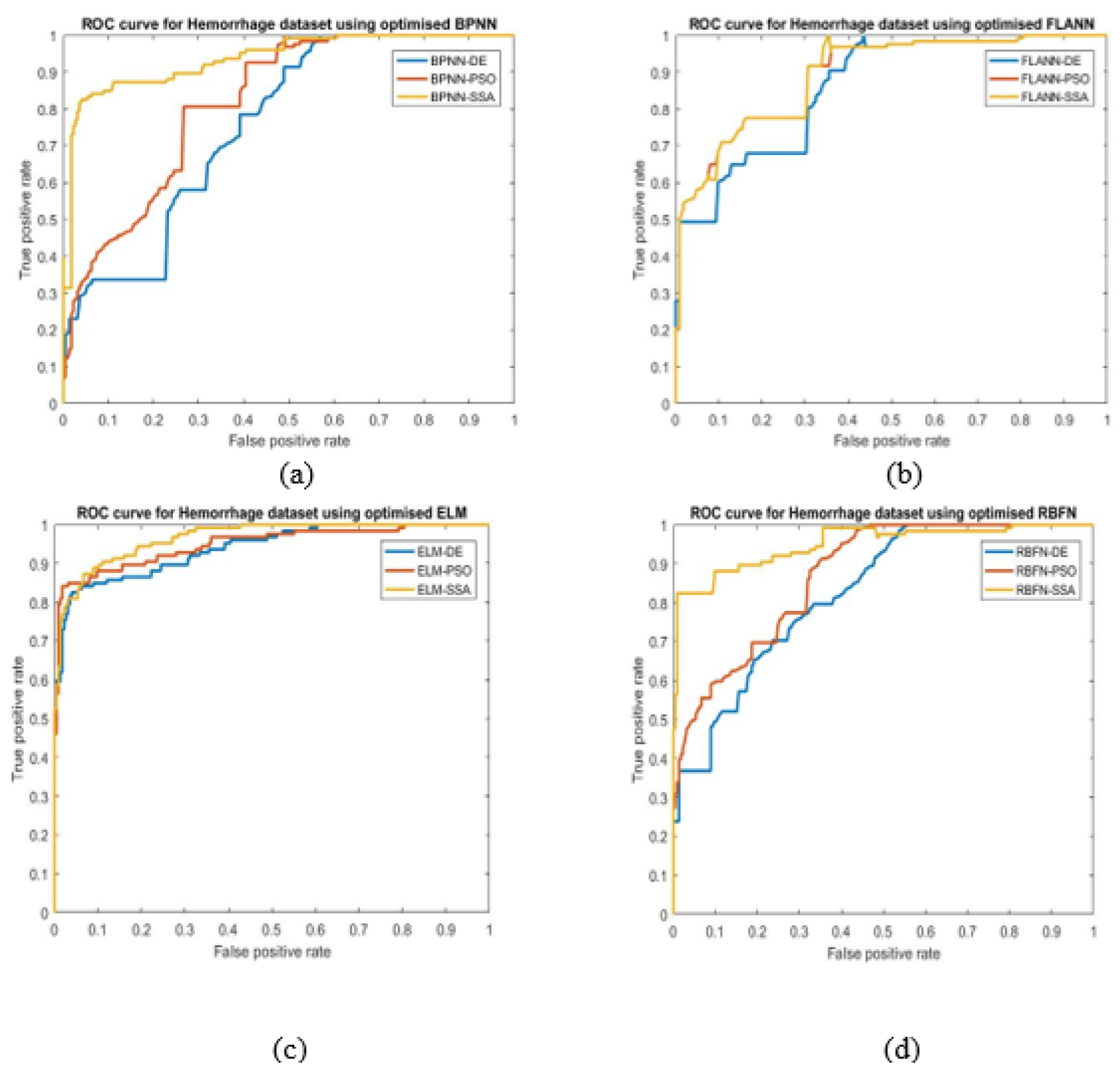
  • ROC: It is an evaluation measure of binary classification and indicate diagnostic ability of classifier. It is a probabilistic plot between true positive rate (TPR) and false positive rate (FPR).
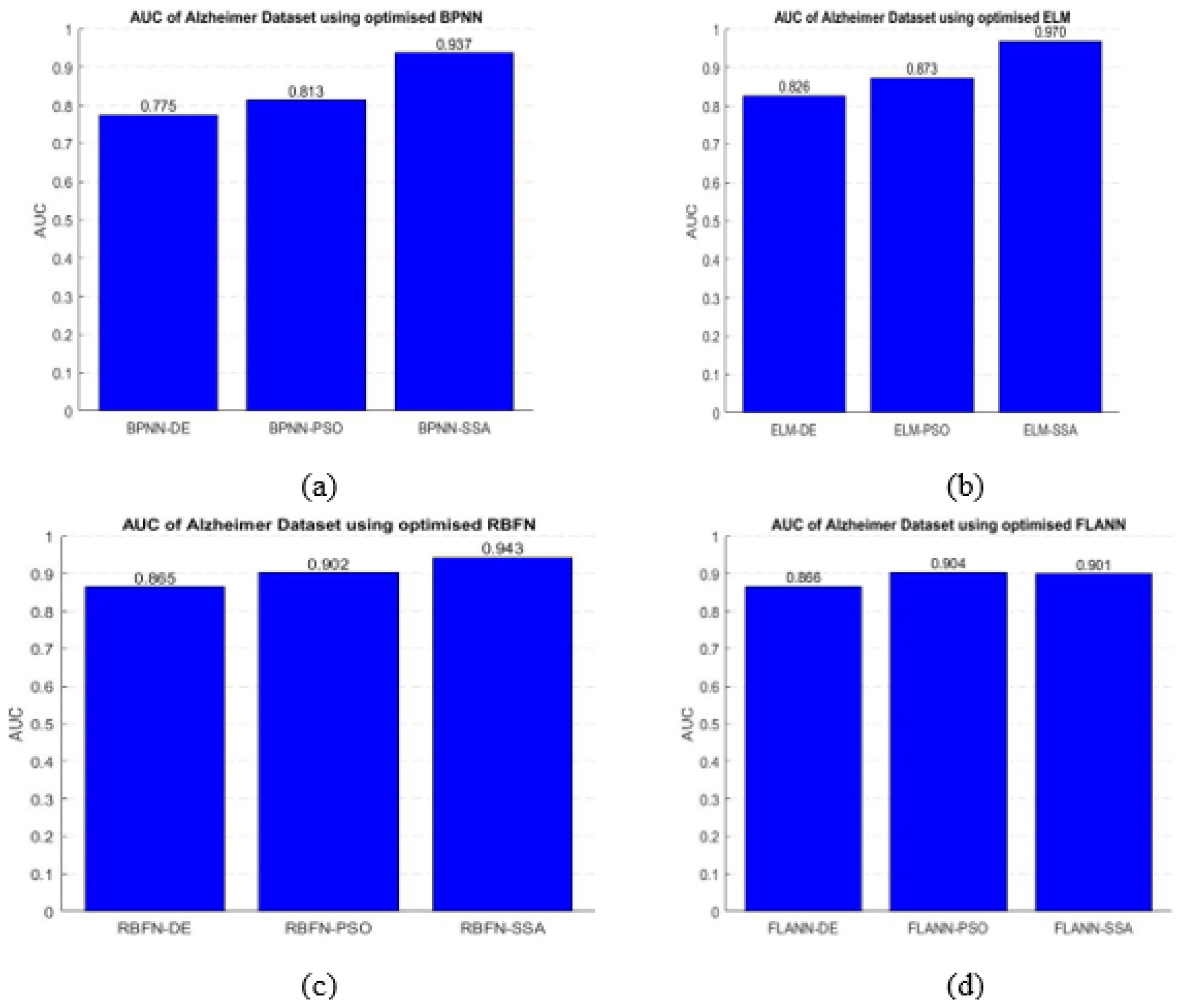
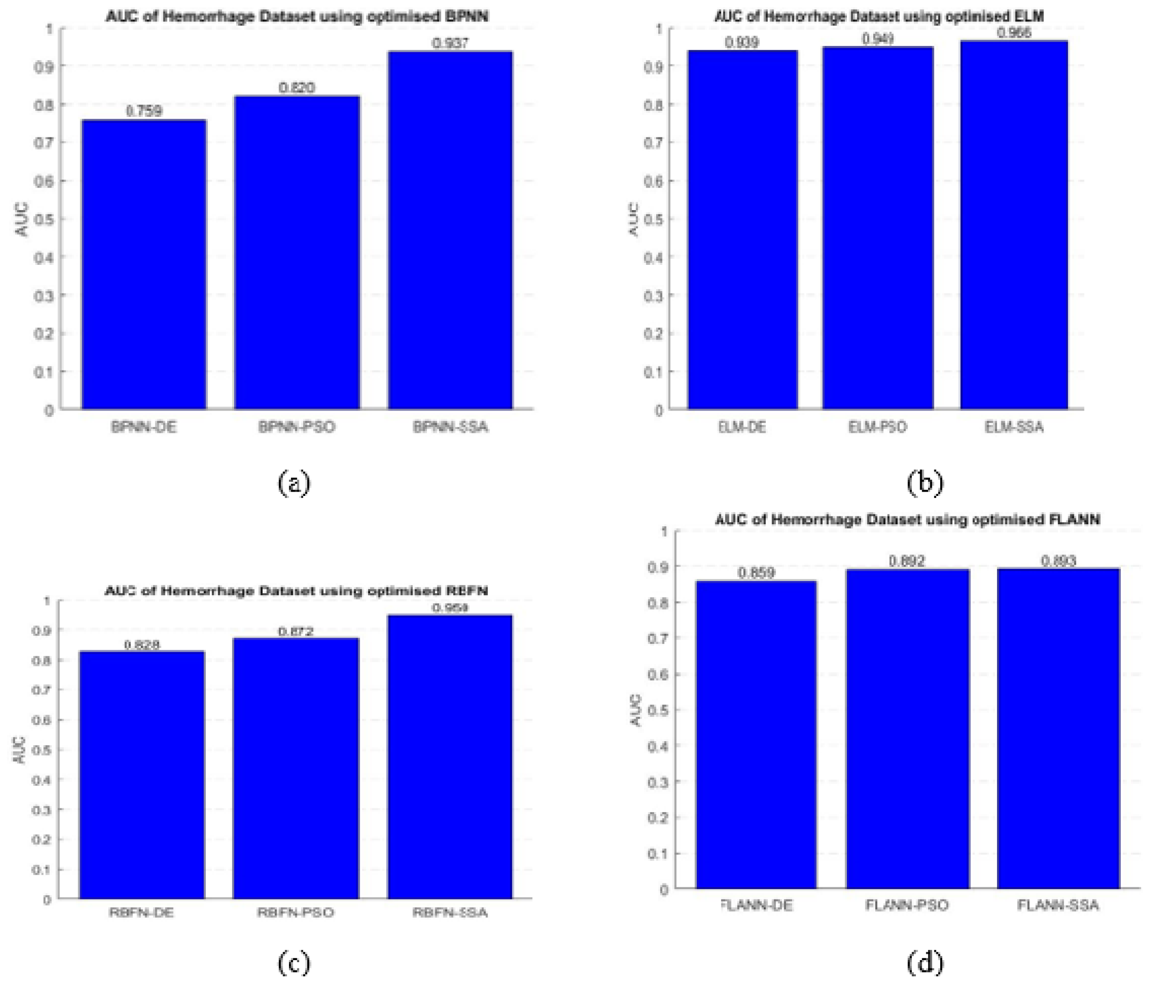
  • AUC: It measures the ability of a classifier to differentiate between classes and represents the summary of the ROC curve. A higher AUC exhibits better between two classes.
  • Overall improvement: It represents the percentage of improvement of the proposed classifier over other classification models in terms of accuracy, AUC, and ROC.
  • Speedup: It measures the relative comparison of execution time without of any standard classifier, which is represented as
    S l a t e n c y = S o l d S n e w
    where S o l d is the execution time of standard classifier, and S n e w is the execution time of proposed hybrid classier.

4.3. Parameters Setting

Each bioinspired algorithm and classifier structure has various parameters which need to be adjusted suitably during training phase. Table 4 represents the parameters used for training. In this study, Gaussian activation function and 10 numbers of hidden nodes have been considered for both RBFN and BPNN, respectively. As FLANN has single-layer architecture, the hidden layer concept is eliminated and the expansion size of this classifier have been considered as 8 for giving better result. There are two common controlling parameters such as crossover and mutation in DE optimization algorithm having values of 0.2 and 0.4, respectively. In case of PSO, the value of first acceleration coefficient is considered as 1.5 and second acceleration coefficient is considered as 2.
In this simulation study, to have a uniform comparison population size of 50, 100 maximum iterations have been considered for all bioinspired algorithms. The first experiment was conducted to decide the appropriate activation function and number of hidden nodes of LSTM structure. Five activation functions—sine, sigmoid, tribas, radbas, and hardlimit—along with 10 to 50 hidden nodes having 5 nodes per increment have been considered in this work. The simulation results reveals that, the best performance is achieved in sigmoid activation function along with 50 numbers of hidden nodes in both the datasets which is shown in Figure 6. To discard the effect of arbitrary inputs to ELM architecture, each experiment was comprised of 20 trials per fold while keeping same hidden nodes and activation functions.

4.4. Features Extraction and Reduction

The initial dimension of each image is 256 × 256 = 65,536. In this work, a 3-level DWT is used for extracting the feature which produces 36 × 36 = 1296 number of features. To further reduce the number of features, PCA has been used to reduce the dimension to 39 and 70 in case of Alzheimer’s and Hemorrhage datasets respectively. The reduced feature is nearly (3%, 5.4%) and (0.05%, 0.1%) of the original dimension for Alzheimer’s and Hemorrhage datasets, respectively. Figure 7 shows the variance concerning the number of Principal Components (PCs). The simulation results of both the datasets demonstrate that, only 39 and 70 PCs maintain more than 95% of the total variance.

4.5. Performance Comparison

The reduced 39 and 70 number of features have been applied four different classifiers such as; ELM, FLANN, RBFN and BPNN. The testing accuracy of base classifiers with conventional learning models has been obtained and shown in Figure 8.
From the above figure, it is observed that the conventional ELM achieves 87% of accuracy in case of Alzheimer’s dataset and 88% of accuracy in case of Hemorrhage dataset, which are superior to accuracy values of other classifiers. To further improve the accuracy, the parameters of four models have been learned using PSO, DE and SSA.
The comparison of accuracy of the hybrid models has been made in Figure 9 and Figure 10 for the two datasets, respectively. By comparing the classification performance of the proposed ELM-SSA (Figure 9b) with others (Figure 9a,c,d) using Alzheimer’s dataset, it is learnt that the ELM-SSA has highest accuracy than other classifiers. It is also observed that ELM-SSA model provide fastest convergence. The SSA based ELM model offers the best convergence speed. Similarly, by comparing the ELM-SSA (Figure 10c) with other classification results (Figure 10a,b,d) for Hemorrhage’s dataset, it can be observed that the ELM-SSA model yields higher accuracy and faster convergence speed. Table 5 presents the comparison of accuracy and AUC of all models. The classification accuracy of the ELM-SSA model obtained for Alzheimer’s and Hemorrhage datasets are found to be 99%. Figure 11 and Figure 12 show the comparison of ROC plots for two datasets using hybrid classifiers. It is observed from the plot that the ROC of ELM-SSA lies closer to y-axis which is true positive rate. Figure 13 and Figure 14 display the comparison plots of AUC for two datasets using hybrid classifiers. From this plot, it is found that the ELM-SSA model provides highest AUCs of 0.9695 and 0.9659 , respectively, for two datasets which are superior to other hybridized models. The performance improvement of ELM-SSA model over other classification models is listed in Table 6.
From Table 6, it is observed that the hybrid classification models which employ optimization techniques provide better accuracy as compared to basic classification models without optimization. Further, ELM-SSA model provides 13.79% and 12.5% better accuracy as compared to basic ELM in case of Alzheimer’s and Hemorrhage datasets, respectively. Similarly, it is demonstrated that the ELM-SSA model outperforms other hybrid ELM models with an improved accuracy of 10%, 3.12% and 8.79%, 3.12% in case of Alzheimer’s and Hemorrhage datasets over the ELM-DE and ELM-PSO models, respectively. The ELM-SSA also exhibits superior classification compared to FLANN, RBFN, and BPNN with enhanced accuracy of 22.22%, 30.26% and 26.92% for Alzheimer’s dataset and 22.22%, 23.75%, and 25.31% for Hemorrhage dataset, respectively. The results of Table 6 also show that ELM-SSA outperforms other hybridized classification models such as FLANN-SSA with increased accuracy of 5.31% and 1.02% for Alzheimer’s and Hemorrhage datasets respectively. Similarly, the ELM-SSA has produced 8.79% and 2.06% better accuracy as compared to RBFN-SSA. ELM-SSA model with 7.6% and 1.02% higher accuracy for Alzheimer’s and Hemorrhage datasets respectively as compared to the BPNN-SSA.
From the analysis of all results, the ELM model with SSA based parameters tuning outperforms the basic ELM, FLANN, RBFN, and BPNN classification models. Further, ELM-SSA also exhibits superior performance over FLANN, RBFN, and BPNN models hybridized with PSO, DE, as well as SSA schemes.
In Table 7, the accuracy of the proposed model has been compared with that obtained from other models in the field for Alzheimer’s and Hemorrhage disease classification. The reported results are 93.18%, 98.01%, 96.36% and 96.50% of accuracy in case of Alzheimer’s dataset [36,37,38,39] and 95.73%, 94.26%, and 95.5% of accuracy in case of Hemorrhage dataset [40,41,42]. In essence, the proposed model have achieved an average improvement accuracy of 4% than previously hybrid classification models.
Table 8 shows the comparison of the overall execution time of the proposed and other hybridized models. It is seen that on an average, the ELM-SSA model yields lower execution time compared to other models.

4.6. Analysis of Computational Time

The computational time of each phase of proposed hybrid classifier (DWT + PCA + ELM-SSA) has been calculated for both the datasets. Figure 15 represents the comparison of the average time required for feature extraction, feature reduction, and classification over both the datasets in seconds (s) for a single brain image having a size of 256 × 256 .
For the Alzheimer’s dataset, each brain MR image takes 0.015 s, 0.004 s, and 0.001 s for feature extraction, feature reduction and in classification, respectively, whereas the corresponding times are 0.014 s, 0.005 s, and 0.0018 s for the Hemorrhage dataset. It has been also found from the above analysis that the overall computational time for processing each MR image of Alzheimer’s and Hemorrhage datasets are 0.0202 s and 0.0205 s, respectively. It is also observed that feature extraction phase consumes more time than either feature reduction and classification steps.
The summary of the investigated is listed in steps:
  • In this work, Alzheimer’s and Hemorrhage brain MRI datasets has been considered and are used for classification with RBFN, FLANN, BPNN, and ELM models.
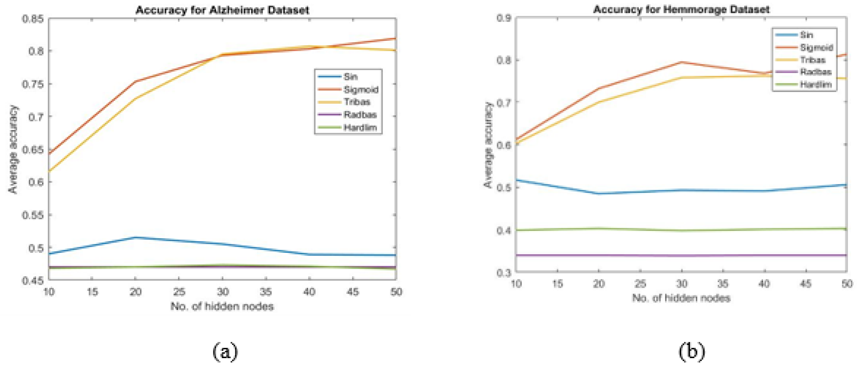
  • The training process of ELM is very simple, but it needs more hidden unit’s comparison to RBFN, FLANN, and BPNN models.
  • The suitable activation function and appropriate number of hidden nodes of ELM are chosen by trial and error. In this work, it is found that, s i g m o i d activation function and 50 numbers of hidden units provide better accuracy than those obtained by other combination.
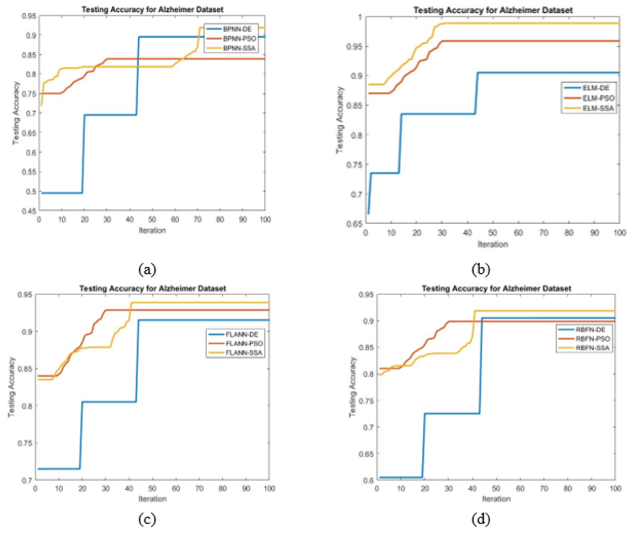
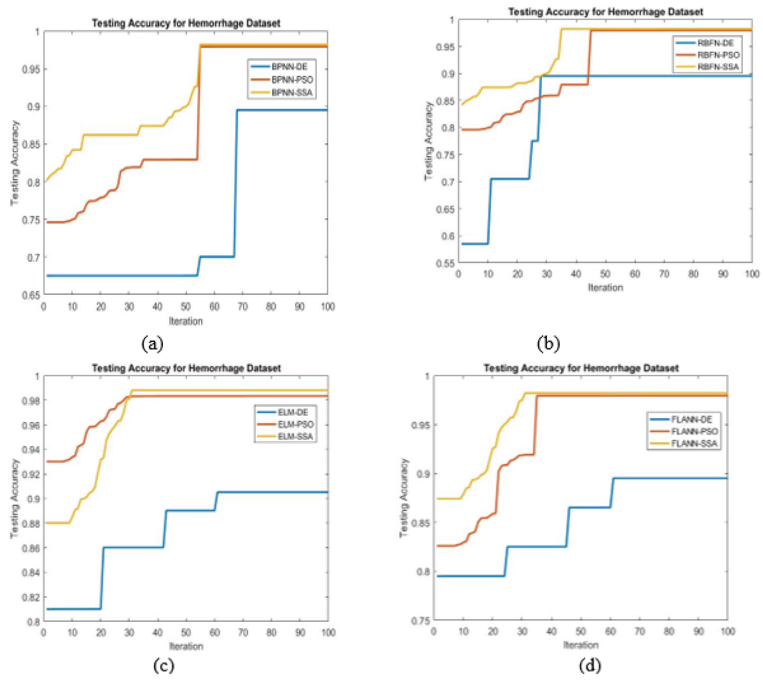
  • For achieving the best possible classification, different bioinspired techniques such as PSO, DE, and SSA have been chosen.
  • To find the maximum accuracy, the SSA tuned ELM classifier is found to be best.
  • For a comparison purpose, same population size and number of iterations are taken in all the evolutionary algorithms
  • Higher classification accuracy is demonstrated by the proposed ELM-SSA approach for the two datasets
  • The highest AUC value is achieved by the ELM-SSA model compared to other hybridized classifier which is true for the two datasets.
  • The ELM-SSA model exhibits the best ROC plots for the two datasets used.
  • In Table 6, it is shown that the ELM-SSA combined model produces better classification accuracy than the basic ELM as well as other classification schemes using FLANN, RBFN, and BPNN models.
  • It is also observed that feature extraction phase consumes more computational time than either of feature reduction and classification stage.
  • In general, the proposed ELM-SSA model outperforms other hybridized classification models such as FLANN-SSA with an improvement in accuracy of 5.31 % and 1.02 % for Alzheimer’s and Hemorrhage datasets respectively. Similarly the ELM-SSA model has produced 8.79 % and 2.06 % better accuracy as compared to RBFN-SSA for two datasets. ELM-SSA has also shown 7.6 % and 1.02 % higher accuracy for Alzheimer’s and Hemorrhage datasets, respectively, as compared to BPNN-SSA.
  • In general, it is found that the proposed ELM-SSA model executes faster than other models over both the datasets.

5. Conclusions and Future Work

The paper has suggested an efficient and faster hybrid classification model using two standard MR image datasets. Through exhaustive simulation study, it is demonstrated that the proposed ELM-SSA model outperforms other competitive conventional and hybrid ML models. A special ongoing favorable metaheuristic optimization algorithm like Salp Swarm Algorithm has been proposed in this work. As the output weight of the learning model depends on arbitrary input weights and biases, it needs to optimize the hidden neuron parameters in ELM for better results. The SSA-based ELM model exhibits parameters tuned. From the above discussion, the ELM-SSA model has shown 13.79 % and 12.5 % improved accuracy as compared to basic ELM model for two datasets. Similarly, the ELM-SSA model also outperforms other hybrid ELM models such as ELM-DE and ELM-PSO with an improved accuracy of 10 % , 3.12 % and 8.79 % , 3.12 % in case of Alzheimer’s and Hemorrhage datasets, respectively. The ELM-SSA also exhibits superior classification compared to FLANN, RBFN, and BPNN with an enhanced accuracy of 22.22%, 30.26%, and 26.92% for Alzheimer’s dataset and 22.22%, 23.75%, and 25.31% for the Hemorrhage dataset, respectively. ELM-SSA outperforms other hybridized classification models such as FLANN-SSA with increased accuracy of 5.31% and 1.02% for Alzheimer’s and Hemorrhage datasets respectively. Similarly, the ELM-SSA has produced 8.79% and 2.06% better accuracy as compared to RBFN-SSA. The proposed model with 7.6% and 1.02% higher accuracy for Alzheimer’s and Hemorrhage datasets, respectively, as compared to the BPNN-SSA. It has been found from the results section that the ELM-SSA model provides the highest AUCs of 0.9695 and 0.9659, respectively, for two datasets which are superior to other hybridized models. The classification accuracy of the ELM-SSA model obtained for both datasets is found to be 99%. It was also found that ELM based hybrid classification model such as ELM-SSA is a better classifier model as compared to FLANN, RBFN, and BPNN classifiers optimized by SSA, PSO, and DE concerning classification accuracy, ROC, and AUC.
In the future, the potentiality of SSA can employed for Kernel ELM (K-ELM) and Regularized ELM model. Classification accuracy can be improve by using different deep learning techniques and ensemble models.The performance of proposed model could be improvised by adding more samples and different augmentation techniques.

Author Contributions

D.M., K.D., S.K. and M.Z. formulated the idea of the study, A.P. and G.P. collected the data and performed the implementation. A.P., D.M. and S.K. wrote the manuscript and checked the English and proofread. A.P. drafted all the figures and tables and prepared the results. All authors have read and agreed to the published version of the manuscript.

Funding

This work was financially supported by the Ministry of Science and Higher Education of the Russian Federation (Government Order) under Grant FENU-k2020-0022.

Institutional Review Board Statement

Not Applicable.

Informed Consent Statement

Not Applicable.

Data Availability Statement

Data available on request.

Acknowledgments

The authors gratefully acknowledge the financial support of the Ministry of Education and Science of the Russian Federation in the framework of Increase Competitiveness Program of NUST MISiS, grant number (K4-2017-052).

Conflicts of Interest

The authors declare no conflict of interest.

References

  1. Mohsin, S.A.; Sheikh, N.M.; Saeed, U. MRI induced heating of deep brain stimulation leads: Effect of the air-tissue interface. Prog. Electromagn. Res. 2008, 83, 81–91. [Google Scholar] [CrossRef] [Green Version]
  2. Zhang, Y.; Dong, Z.; Wu, L.; Wang, S. A hybrid method for MRI brain image classification. Expert Syst. Appl. 2011, 38, 10049–10053. [Google Scholar] [CrossRef]
  3. Chaplot, S.; Patnaik, L.M.; Jagannathan, N.R. Classification of magnetic resonance brain images using wavelets an input to support vector machine and neural network. Biomed. Signal Process. Control 2006, 1, 86–92. [Google Scholar] [CrossRef]
  4. Maitra, M.; Chatterjee, A. A Slantlet transform based intelligent system for magnetic resonance brain image classification. Biomed. Signal Process. Control 2006, 1, 299–306. [Google Scholar] [CrossRef]
  5. Das, S.; Chowdhury, M.; Kundu, M.K. Brain MR image classification using multiscale geometric analysis of ripplet. Prog. Electromagn. Res. 2013, 137, 1–17. [Google Scholar] [CrossRef] [Green Version]
  6. Eshtay, M.; Faris, H.; Obeid, N. Metaheuristic-based extreme learning machines: A review of design formulations and applications. Int. J. Mach. Learn. Cybern. 2019, 10, 1543–1561. [Google Scholar] [CrossRef]
  7. Mirjalili, S.; Gomi, A.H.; Mirjalili, S.Z.; Saremi, S.; Faris, H.; Mirjalili, S.M. Salp Swarm Algorithm: A bio-inspired optimizer for engineering design problems. Adv. Eng. Softw. 2017, 114, 163–191. [Google Scholar] [CrossRef]
  8. Aljarah, I.; Faris, H.; Mirjalili, S.; Al-Madi, N. Training radial basis function networks using a biogeography-based optimizer. Neural Comput. Appl. 2018, 29, 529–553. [Google Scholar] [CrossRef]
  9. Faris, H.; Aljarah, I.; Mirjalili, S. Training feedforward neural networks using multi-verse optimizer for binary classification problems. Appl. Intell. 2016, 45, 322–332. [Google Scholar] [CrossRef]
  10. Mansour, R.F.; Escorcia-Gutierrez, J.; Gamarra, M.; Díaz, V.G.; Gupta, D.; Kumar, S. Artificial intelligence with big data analytics-based brain intracranial hemorrhage e-diagnosis using CT images. Neural Comput. Appl. 2021, 1–13. [Google Scholar] [CrossRef]
  11. Ding, S.; Su, C.; Yu, J.S. An optimizing BP neural network algorithm based on genetic algorithm. Artif. Intell. Rev. 2011, 36, 153–162. [Google Scholar] [CrossRef]
  12. DGori, M.; Tesi, A. On the problem of local minima in backpropagation. IEEE Trans. Pattern Anal. Mach. Intell. 1992, 1, 76–86. [Google Scholar] [CrossRef] [Green Version]
  13. Gupta, J.N.; Sexton, R.S. Comparing backpropagation with a genetic algorithm for neural network training. Omega 1999, 27, 679–684. [Google Scholar] [CrossRef]
  14. Sexton, R.S.; Dorsey, R.E.; Johnson, J.D. Optimization of neural networks: A comparative analysis of the genetic algorithm and simulated annealing. Eur. J. Oper. Res. 1999, 114, 589–601. [Google Scholar] [CrossRef]
  15. Huang, G.B.; Zhu, Q.Y.; Siew, C.K. Extreme learning machine: A new learning scheme of feedforward neural networks. In Proceedings of the 2004 IEEE International Joint Conference on Neural Networks (IEEE Cat. No. 04CH37541), Budapest, Hungary, 25–29 July 2004; pp. 985–990. [Google Scholar]
  16. El-Dahshan, E.S.A.; Hosny, T.; Salem, A.B.M. Hybrid intelligent techniques for MRI brain images classification. Digit. Signal Process. 2010, 20, 433–441. [Google Scholar] [CrossRef]
  17. Aljarah, I.; Ala’M, A.Z.; Faris, H.; Hassonah, M.A.; Mirjalili, S.; Saadeh, H. Simultaneous feature selection and support vector machine optimization using the grasshopper optimization algorithm. Cogn. Comput. 2018, 10, 478–441. [Google Scholar] [CrossRef] [Green Version]
  18. Mafarja, M.; Aljarah, I.; Heidari, A.A.; Hammouri, A.I.; Faris, H.; Ala’M, A.Z.; Mirjalili, S. Evolutionary population dynamics and grasshopper optimization approaches for feature selection problems. Knowl.-Based Syst. 2018, 145, 25–45. [Google Scholar] [CrossRef] [Green Version]
  19. Xu, Y.; Shu, Y. Evolutionary extreme learning machine–based on particle swarm optimization. In International Symposium on Neural Networks; Springer: Berlin/Heidelberg, Germany, 2006; pp. 644–652. [Google Scholar]
  20. Yang, Z.; Wen, X.; Wang, Z. QPSO-ELM: An evolutionary extreme learning machine based on quantum-behaved particle swarm optimization. In Proceedings of the 2015 Seventh International Conference on Advanced Computational Intelligence (ICACI), Wuyi, China, 27–29 March 2015; pp. 69–72. [Google Scholar]
  21. El-Dahshan, E.S.A.; Mohsen, H.M.; Revett, K.; Salem, A.B.M. Computer-aided diagnosis of human brain tumor through MRI: A survey and a new algorithm. Expert Syst. Appl. 2014, 41, 5526–5545. [Google Scholar] [CrossRef]
  22. Dehuri, S.; Roy, R.; Cho, S.B.; Ghosh, A. An improved swarm optimized functional link artificial neural network (ISO-FLANN) for classification. J. Syst. Softw. 2012, 85, 1333–1345. [Google Scholar] [CrossRef]
  23. Ma, C. An Efficient Optimization Method for Extreme Learning Machine Using Artificial Bee Colony. J. Digit. Inf. Manag. 2017, 15, 135–147. [Google Scholar]
  24. Eusuff, M.M.; Lansey, K.E. Optimization of water distribution network design using the shuffled frog leaping algorithm. J. Water Resour. Plan. Manag. 2003, 129, 210–225. [Google Scholar] [CrossRef]
  25. Eusuff, M.; Lansey, K.; Pasha, F. Shuffled frog-leaping algorithm: A memetic meta-heuristic for discrete optimization. Eng. Optim. 2006, 38, 129–154. [Google Scholar] [CrossRef]
  26. Luo, J.P.; Li, X.; Chen, M.R. Hybrid shuffled frog leaping algorithm for energy-efficient dynamic consolidation of virtual machines in cloud data centers. Expert Syst. Appl. 2014, 41, 5804–5816. [Google Scholar] [CrossRef]
  27. Nejad, M.B.; Ahmadabadi, M.E.S. A novel image categorization strategy based on salp swarm algorithm to enhance efficiency of MRI images. Comput. Model. Eng. Sci. 2019, 119, 185–205. [Google Scholar]
  28. Huang, Y.W.; Lai, D.H. Hidden node optimization for extreme learning machine. Aasri Procedia 2012, 3, 375–380. [Google Scholar] [CrossRef]
  29. Xiao, D.; Li, B.; Mao, Y. A multiple hidden layers extreme learning machine method and its application. Math. Probl. Eng. 2017, 2017, 4670187. [Google Scholar] [CrossRef]
  30. Yang, Y.; Wu, Q.J.; Wang, Y.; Mukherjee, D.; Chen, Y. ELM Feature Mappings Learning: Single-Hidden-Layer Feedforward Network without Output Weight. In Proceedings of ELM-2014 Volume 1; Springer: Berlin/Heidelberg, Germany, 2015; pp. 311–324. [Google Scholar]
  31. Setiawan, A.W.; Mengko, T.R.; Santoso, O.S.; Suksmono, A.B. Color retinal image enhancement using CLAHE. In Proceedings of the International Conference on ICT for Smart Society, Jakarta, Indonesia, 13–14 June 2013; pp. 1–3. [Google Scholar]
  32. Reza, A.M. Realization of the contrast limited adaptive histogram equalization (CLAHE) for real-time image enhancement. J. VLSI Signal Process. Syst. Signal Image Video Technol. 2004, 38, 35–44. [Google Scholar] [CrossRef]
  33. Reddy, A.V.N.; Krishna, C.P.; Mallick, P.K.; Satapathy, S.K.; Tiwari, P.; Zymbler, M.; Kumar, S. Analyzing MRI scans to detect glioblastoma tumor using hybrid deep belief networks. J. Big Data 2020, 7, 1–17. [Google Scholar] [CrossRef]
  34. Ma, J.; Yuan, Y. Dimension reduction of image deep feature using PCA. J. Vis. Commun. Image Represent. 2019, 63, 102578. [Google Scholar] [CrossRef]
  35. Faris, H.; Mirjalili, S.; Aljarah, I.; Mafarja, M.; Heidari, A.A. Salp swarm algorithm: Theory, literature review, and application in extreme learning machines. Nat.-Inspired Optim. 2020, 185–199. [Google Scholar] [CrossRef]
  36. Islam, J.; Zhang, Y. Brain MRI analysis for Alzheimer’s disease diagnosis using an ensemble system of deep convolutional neural networks. Brain Inform. 2018, 5, 1–14. [Google Scholar] [CrossRef]
  37. Goceri, E. Diagnosis of Alzheimer’s disease with Sobolev gradient-based optimization and 3D convolutional neural network. Int. J. Numer. Methods Biomed. Eng. 2019, 35, e3225. [Google Scholar] [CrossRef] [PubMed]
  38. Khan, N.M.; Abraham, N.; Hon, M. Transfer learning with intelligent training data selection for prediction of Alzheimer’s disease. IEEE Access 2019, 7, 72726–72735. [Google Scholar] [CrossRef]
  39. Farid, A.A.; Selim, G.I.; Khater, H.A.A. Applying artificial intelligence techniques to improve clinical diagnosis of Alzheimer’s disease. Eur. J. Eng. Sci. Technol. 2020, 3, 58–79. [Google Scholar] [CrossRef]
  40. Anupama, C.S.S.; Sivaram, M.; Lydia, E.L.; Gupta, D.; Shankar, K. Synergic deep learning model–based automated detection and classification of brain intracranial hemorrhage images in wearable networks. Pers. Ubiquitous Comput. 2020, 1–10. [Google Scholar] [CrossRef]
  41. Kirithika, R.A.; Sathiya, S.; Balasubramanian, M.; Sivaraj, P. Brain Tumor And Intracranial Haemorrhage Feature Extraction And Classification Using Conventional and Deep Learning Methods. Eur. J. Mol. Clin. Med. 2020, 7, 237–258. [Google Scholar]
  42. Nawresh, A.A.; Sasikala, S. An Approach for Efficient Classification of CT Scan Brain Haemorrhage Types Using GLCM Features with Multilayer Perceptron; ICDSMLA 2019; Springer: Berlin/Heidelberg, Germany, 2020; pp. 400–412. [Google Scholar]
Figure 1. Filter bank approach of 2D-DWT for MR image synthesis.
Mathematics 09 02095 g001
Figure 2. Schematic structure of ELM model.
Mathematics 09 02095 g002
Figure 3. Samples of brain MR image: (a) Normal MRI. (b) Alzheimer’s disease. (c) Hemorrhage’s disease.
Mathematics 09 02095 g003
Figure 4. Model for propose ELM-SSA classification of MR brain images.
Mathematics 09 02095 g004
Figure 5. Vector structure of salp in ELM-SSA.
Mathematics 09 02095 g005
Figure 6. Comparison of average accuracy of five different activation functions along with the number of hidden neurons used in ELM: (a) Alzheimer’s dataset and (b) Hemorrhage dataset.
Mathematics 09 02095 g006
Figure 7. Variance (%) in respect of the number of PCs for both (a) Alzheimer’s and (b) Hemorrhage dataset.
Mathematics 09 02095 g007
Figure 8. Comparison of testing accuracy of detection using Alzheimer’s and Hemorrhage datasets to ELM, FLANN, RBFN, and BPNN.
Mathematics 09 02095 g008
Figure 9. Comparison of Accuracy of classification of Alzheimer’s dataset using (a) BPNN, (b) ELM, (c) FLANN, or (d) RBFN.
Mathematics 09 02095 g009
Figure 10. Comparison of Accuracy of Hemorrhage dataset using (a) BPNN, (b) RBFN, (c) ELM, ir (d) FLANN.
Mathematics 09 02095 g010
Figure 11. Comparison of ROC plots for Alzheimer’s dataset using classifier (a) BPNN, (b) ELM, (c) RBFN, or (d) FLANN.
Mathematics 09 02095 g011
Figure 12. Comparison of ROC plots for Hemorrhage dataset using classifiers (a) BPNN, (b) FLANN, (c) ELM, or (d) RBFN.
Mathematics 09 02095 g012
Figure 13. Comparison of AUC values for Alzheimer’s dataset obtained using models (a) BPNN, (b) ELM, (c) RBFN, or (d) FLANN.
Mathematics 09 02095 g013
Figure 14. Comparison of AUC values for Hemorrhage dataset from models (a) BPNN, (b) ELM, (c) RBFN, or (d) FLANN.
Mathematics 09 02095 g014
Figure 15. Average computational time in (second) at different phases of ELM-SSA over Alzheimer’s and Hemorrhage datasets.
Mathematics 09 02095 g015
Table 1. Datasets specification.
DatasetNo. of InstancesImage FormatImage SizeClassesSample TypeNo. of AttributeAttributes after PCA
Alzheimer’s100BMP 256 × 256 2T2-weighted129639
Hemorrhage200JPEG 256 × 256 2T1-weighted129670
Table 2. Details of 5 × 5 -fold stratified cross-validation scheme used.
DatasetTotal Number of ImagesNumber of Normal Training ImagesNumber of Abnormal Training ImagesNumber of Normal Testing ImagesNumber of Abnormal Testing Images
Alzheimer’s10040401010
Hemorrhage20080802020
Table 3. The detailed configuration of the utilized system.
Name (Hardware/Software)Setting
CPUIntel(R) Core(TM) i3-6006U
Frequency2.0 GHz
RAM8 GB
Hard Drive500 GB
Operating SystemWindow 7
Simulation softwareMat lab R2015a
Table 4. Various parameter values used during model development.
ELMRBFNFLANNBPNNPSODESSA
Hidden layer size: 50, Activation function: sigmoidBasis function: Gaussian,Hidden layer size: 10, Learning rate: 0.5Size of expansion: 8Learning rate: 0.9, Momentum: 0.3, Hidden layer size: 10, Activation function: GaussianIteration: 100, Population Size: 50, Inertia Weight (IW): 0.7, Inertia Weight Damping Ratio: 0.1, ( c 1 ) : 1.5, ( c 2 ) : 2Iteration: 100, Population Size: 50, Crossover: 0.2, Mutation: 0.4, LB: 0.25, UB: 0.75Iteration: 100, Population Size: 50, Inertia weight: 0.7
Table 5. Comparison of Accuracy and AUC of hybrid models using Alzheimer’s and Hemorrhage datasets.
MethodsAccuracy (Alzheimer’s)AUC (Alzheimer’s)Accuracy (Hemorrhage)AUC (Hemorrhage)
ELM-SSA0.990.96950.990.9659
ELM-PSO0.960.87310.960.9489
ELM-DE0.900.82610.910.9393
FLANN-SSA0.940.90070.980.8929
FLANN-PSO0.930.90390.970.8924
FLANN-DE0.910.86580.890.8591
RBFN-SSA0.910.94330.970.9501
RBFN-PSO0.890.90190.960.8722
RBFN-DE0.900.86500.890.8275
BPNN-SSA0.920.93730.980.9373
BPNN-PSO0.830.81340.970.8204
BPNN-DE0.890.77530.960.7590
Table 6. Performance comparison of ELM-SSA model with other classification models.
MethodsClassification Accuracy (Alzheimer’s Dataset) Performance Improvement of ELM-SSA (%)Classification Accuracy (Hemorrhage Dataset)Performance Improvement of ELM-SSA (%)
ELM0.8713.790.8812.5
ELM-PSO0.963.120.963.12
ELM-DE0.90100.918.79
FLANN0.8122.220.8122.22
FLANN-SSA0.945.310.981.02
FLANN-PSO0.936.40.972.06
FLANN-DE0.918.790.8911.23
RBFN0.7630.260.8023.75
RBFN-SSA0.918.790.972.06
RBFN-PSO0.8911.230.963.12
RBFN-DE0.90100.8911.23
BPNN0.7826.920.7925.31
BPNN-SSA0.927.60.981.02
BPNN-PSO0.8319.270.972.06
BPNN-DE0.8911.230.963.12
Table 7. Comparison of classification Accuracy of ELM-SSA model with other models using Alzheimer’s and Hemorrhage Datasets.
PaperClassifier (Techniques)Accuracy (%) of Alzheimer’s DatasetAccuracy (%) of Hemorrhage Dataset
[36]Res-Net93.18-
[37]3D-CNN98.01-
[38]VGG96.36-
[39]SVM(CHFS)96.50-
[40]CNN(GC-SDL)-95.73
[41]Alex Net(CLAHE+SITF)-94.26
[42]K-NN(GLCM)-95.5
[42]Multilayer Perceptron (GLCM)-95.5
Proposed modelELM-SSA (DWT+PCA)9999
Table 8. Comparison of average execution time of proposed ELM-SSA model with other classification models.
ModelsTotal Execution Time (Second) (Alzheimer’s Dataset)Speedup of ELM-SSATotal Execution Time (Second) (Hemorrhage Dataset)Speedup of ELM-SSA
ELM7001.06×7801.03×
ELM-SSA660-755-
ELM-PSO7101.07×7901.04×
ELM-DE7251.09×8001.05×
FLANN7201.09×8101.07×
FLANN-SSA7451.12×8501.12×
FLANN-PSO6801.03×8441.11×
FLANN-DE7551.14×8901.17×
RBFN7581.14×8401.10×
RBFN-SSA7651.15×9101.20×
RBFN-PSO7901.19×9401.24×
RBFN-DE7771.17×9551.26×
BPNN7651.15×8801.16×
BPNN-SSA8101.22×9101.20×
BPNN-PSO8851.34×9051.19×
BPNN-DE8801.33×9101.20×
Publisher’s Note: MDPI stays neutral with regard to jurisdictional claims in published maps and institutional affiliations.

