Point Cloud Registration Based on Multiparameter Functional

Abstract

The registration of point clouds in a three-dimensional space is an important task in many areas of computer vision, including robotics and autonomous driving. The purpose of registration is to find a rigid geometric transformation to align two point clouds. The registration problem can be affected by noise and partiality (two point clouds only have a partial overlap). The Iterative Closed Point (ICP) algorithm is a common method for solving the registration problem. Recently, artificial neural networks have begun to be used in the registration of point clouds. The drawback of ICP and other registration algorithms is the possible convergence to a local minimum. Thus, an important characteristic of a registration algorithm is the ability to avoid local minima. In this paper, we propose an ICP-type registration algorithm ($\lambda$-ICP) that uses a multiparameter functional ($\lambda$-functional). The proposed $\lambda$-ICP algorithm generalizes the NICP algorithm (normal ICP). The application of the $\lambda$-functional requires a consistent choice of the eigenvectors of the covariance matrix of two point clouds. The paper also proposes an algorithm for choosing the directions of eigenvectors. The performance of the proposed $\lambda$-ICP algorithm is compared with that of a standard point-to-point ICP and neural network Deep Closest Points (DCP).

1. Introduction

Point cloud registration is a key element in the reconstruction of a 3D spatial environment for robots and sensors. Point cloud registration means finding an orthogonal transformation in $R^3$ that maximizes a consistent overlap between two clouds. The iterative closest points algorithm (ICP) [1,2] is the most known algorithm for registering point clouds. The two basic steps of the ICP algorithm alternate with each other, that is, the estimation of the geometric transformation based on a fixed correspondence (variational problem of the ICP algorithm) and updating the correspondences to their closest matches (matching step).

The most famous functionals used in the variational problem are presented in various ICP variants; that is, point-to-point [1], point-to-plane [2], generalized ICP [3] and normal ICP (NICP) [4,5]. In [6], a closed-form solution to the point-to-point affine problem is described. Closed-form solutions to the affine point-to-plane problem are suggested [7,8]. Closed-form solutions to the point-to-point problem in the class of orthogonal transformations are obtained [9,10,11].

More robust ICP algorithms with other functionals have also been proposed, which are called generalized ICP [4] and NICP [5]. The corresponding variational problems are solved using the iterative conjugate gradients and Gauss–Newton methods [4,5].

The variational ICP problem can be solved not only by deterministic, but also by stochastic methods. One of them is the Grey Wolf Optimizer (GWO) algorithm. Recently, GWO has been applied to a rough point clouds alignment [12] and to the realization of the point-to-point ICP algorithm [13].

Usually, the ICP algorithm monotonically reduces functional values, but owing to the problem non-convexity, the algorithm often stops at suboptimal local minima. Thus, the probability of obtaining an acceptable transformation as a result of the ICP algorithm is a comparative criterion for different types of ICP algorithms and other types of registration algorithms.

The paper [4] presents an experimental comparative analysis of the NICP algorithm, generalized ICP, NDT [14] and KinFu [15]. The analysis shows that the NICP yields better results and a higher robustness compared to the state-of-the-art methods [4]. A closed-form solution to the NICP variational problem is proposed [5]. A comparative analysis of the Gauss–Newton iterative method [4] and the closed-form solution to the NICP variational problem are also obtained [5].

Recently, neural network-based approaches have been proposed for point cloud classification, segmentation and shape matching [16,17,18]. Methods for registering point clouds using neural networks have also been recently suggested [18,19,20]. In particular, an efficient neural network approach referred to as Deep Closest Points (DCP) was applied to the problem of registering point clouds [21]. The DCP neural network implements the main steps of the ICP algorithm. The DCP algorithm maps input point clouds with permutations/rigid-invariant embedding that help identify matching pairs of points; the attention-based module then predicts a soft match between the point clouds; finally, the differentiable singular value decomposition layer predicts the rigid transformation [21]. DCP is trained on the ModelNet40 3D point clouds database [22]. In [21], a comparative analysis of the DCP, ICP and PointNetLK neural network [23] algorithms was carried out.

The complexity of the registration task depends on the features of the source and target point clouds. If the point clouds are congruent, then we have a relatively simpler registration problem than in the case of non-congruent clouds.

Note that in real-world applications, a registration algorithm must deal with non-congruent point clouds. An important part of comparing registration algorithms is their evaluation on non-congruent clouds. An easy way to obtain a pair of non-congruent clouds is to add noise.

In this paper, we propose an ICP variational problem based on the functional which we call $\lambda$-functional. Accordingly, the version of ICP described here is referred to as $\lambda$-ICP. The proposed $\lambda$-functional is a generalization of the NICP functional [4,5]. The NICP functional requires the computation of the covariance matrix in the neighborhood of each point in the cloud. The functional includes an information matrix associated with the covariance matrix. The covariance matrix is factorized by the eigenvalue decomposition into the product of orthogonal eigenvector matrices and a diagonal eigenvalue matrix. The information matrix coincides with the covariance matrix or differs from it by the diagonal elements in the eigenvalue matrix.

In [5], it was noted that the selection of diagonal elements for a given point cloud increases the probability of NICP convergence to an acceptable solution. The application of the proposed $\lambda$-functional is based on this observation. The following method is proposed to solve the $\lambda$-ICP variational problem. First, we find a solution to the variational problem in the GL (3) class. Second, we project the obtained result onto the submanifold $SO(3)$ in $R^9$. Finally, the translation vector is calculated. These three steps provide a closed-form solution to the variational problem of the $\lambda$-ICP algorithm that approximates the exact solution. A similar approximation method is used for the point-to-plane ICP [24] and NICP [5].

It is known that conventional eigenvalue decomposition algorithms provide eigenvectors with unpredictable directions [25,26]. The method proposed in [26] reorients each eigenvector so that its sign is coherent with the majority of the vectors. Note that the correct choice of directions of the eigenvectors is critical for the correct work of the $\lambda$-ICP algorithm. In this paper, we propose an algorithm for reorienting eigenvectors that are computed in a neighborhood within a point cloud. We call this algorithm “direction predictor”.

Using a computer simulation, we show that the proposed $\lambda$-ICP algorithm converges well to a suitable orthogonal transformation for a wide class of regularization tasks.

The paper is organized as follows: In Section 2, we propose a closed-form approximation of the exact solution to the variation problem with $\lambda$-functional. In Section 3, we describe the direction predictor algorithm. In Section 4, computer simulation results are presented and discussed. Section 5 summarizes our conclusions.

2. $\mathit{\lambda }$-Functional and Its Minimization

2.1. Information Matrices

Let $P=\{p_1,\dots ,p_s\}$ be a source point cloud, and $Q=\{q_1,\dots ,q_s\}$ be a target point cloud in $R^3$. Suppose that the relation between points of P and Q is given in such a manner that for each point $p_i$ there is a corresponding point $q_i$.

The information matrices were introduced in [4]. Information matrices had a size of $3\times 3$ and were symmetric. Let us consider the k-neighborhood $\{p_i^1,\dots ,p_i^k\}$ of a point $p_i\in P$, $i=1,\dots ,s$. The mass center $\widehat{p_i}$ of the neighborhood and the covariance ${\mathsf{\Sigma }}_i$ were calculated as follows:

$$\widehat{p_i}=\frac{1}{k}\sum _{j=1}^k{p}_i^j,$$

(1)

$${\mathsf{\Sigma }}_i=\frac{1}{k}\sum _{j=1}^k{(p_i^j-\widehat{p_i})}^t(p_i^j-\widehat{p_i}).$$

(2)

The eigendecomposition of the matrix ${\mathsf{\Sigma }}_i$ was calculated as:

$${\mathsf{\Sigma }}_i={\Re }_i\left(\begin{array}{ccc}{\lambda }_1& 0& 0\\ 0& {\lambda }_2& 0\\ 0& 0& {\lambda }_3\end{array}\right){\Re }_i^t,$$

(3)

where ${\lambda }_1$, ${\lambda }_2$, ${\lambda }_3$ are the eigenvalues of ${\mathsf{\Sigma }}_i$ in ascending order, ${\Re }_i$ is the orthogonal matrix of eigenvectors. We defined here an information matrix ${\mathsf{\Omega }}_i^p$ of point $p_i\in P$ as:

$${\mathsf{\Omega }}_i^p={\Re }_i{\mathsf{\Lambda }}_i{\Re }_i^t,$$

(4)

where ${\mathsf{\Lambda }}_i=diag({\lambda }_1,{\lambda }_2,{\lambda }_3)$. We considered ${\lambda }_1$, ${\lambda }_2$, ${\lambda }_3$ as variable parameters. These parameters were selected individually for a given point cloud.

The information matrices ${\mathsf{\Omega }}_i^q$ for point cloud Q were defined similarly.

Denote the surfaces constructed from clouds P and Q by $S(P)$ and $S(Q)$, respectively. Let $T_P(p_i)$ and $T_Q(q_i)$ be the tangent planes of $S(P)$ and $S(Q)$ at points $p_i$ and $q_i$, respectively. Let $n_i^p$ and $n_i^q$ be the normal vectors to the planes $T_P(p_i)$ and $T_Q(q_i)$, respectively, $i=1,\dots ,s$. The normal information matrices ${\mathsf{\Omega }}_i^n$ for the cloud Q were defined in the same way as the information matrices ${\mathsf{\Omega }}_i^q$.

2.2. NICP Functional and Its Decomposition

Denote by $J_{\mathsf{\Omega }}$ the following functional:

$$\begin{array}{c}\hfill J_{\mathsf{\Omega }}(R,T)=\sum _{i=1}^s{(R{p}_i+T-q_i)}^t{\mathsf{\Omega }}_i^q(R{p}_i+T-q_i)+\sum _{i=1}^s{(R{n}_i^p-n_i^q)}^t{\mathsf{\Omega }}_i^n(R{n}_i^p-n_i^q),\end{array}$$

(5)

where ${\mathsf{\Omega }}^p=\{{\mathsf{\Omega }}_1^p,\dots {\mathsf{\Omega }}_s^p\}$ and ${\mathsf{\Omega }}^n=\{{\mathsf{\Omega }}_1^n,\dots {\mathsf{\Omega }}_s^n\}$ are point information and normal information matrices, respectively.

$J_{\mathsf{\Omega }}(R,T)$ is the NICP functional [4,5].

Let us consider the first term of the functional $J_{\mathsf{\Omega }}$. Denote the vector $R{p}_i+T-q_i$ and its coordinates as $v_i={(v_i^1{v}_i^2{v}_i^3)}^t$. The term can be rewritten as: -4.6cm0cm

$$\begin{array}{c}\hfill \sum _{i=1}^s(v_i^1{v}_i^2{v}_i^3){\mathsf{\Omega }}_i^q\left(\begin{array}{c}{v}_i^1\\ v_i^2\\ v_i^3\end{array}\right)=\sum _{i=1}^s(v_i^1{v}_i^2{v}_i^3){\Re }_i{\mathsf{\Lambda }}_i{\Re }_i^t\left(\begin{array}{c}{v}_i^1\\ v_i^2\\ v_i^3\end{array}\right)=\\ \hfill \sum _{i=1}^s(v_i^1{v}_i^2{v}_i^3){\Re }_i\sqrt{{\mathsf{\Lambda }}_i}\sqrt{{\mathsf{\Lambda }}_i}{\Re }_i^t\left(\begin{array}{c}{v}_i^1\\ v_i^2\\ v_i^3\end{array}\right)=\sum _{i=1}^s(v_i^1{v}_i^2{v}_i^3){\Re }_i\sqrt{{\mathsf{\Lambda }}_i}{(\sqrt{{\mathsf{\Lambda }}_i})}^t{\Re }_i^t\left(\begin{array}{c}{v}_i^1\\ v_i^2\\ v_i^3\end{array}\right)=\\ \hfill \sum _{i=1}^s((v_i^1{v}_i^2{v}_i^3){\Re }_i\sqrt{{\mathsf{\Lambda }}_i}){((v_i^1{v}_i^2{v}_i^3){\Re }_i\sqrt{{\mathsf{\Lambda }}_i})}^t=\sum _{i=1}^s<(v_i^1{v}_i^2{v}_i^3){\Re }_i\sqrt{{\mathsf{\Lambda }}_i},(v_i^1{v}_i^2{v}_i^3){\Re }_i\sqrt{{\mathsf{\Lambda }}_i}>,\end{array}$$

(6)

where $\sqrt{{\mathsf{\Lambda }}_i}=diag(\sqrt{{\mathsf{\Lambda }}_{i1}},\sqrt{{\mathsf{\Lambda }}_{i2}},\sqrt{{\mathsf{\Lambda }}_{i3}})$. Denote by $r_{i1}$, $r_{i2}$ and $r_{i3}$ columns of the matrix ${\Re }_i$. Consider the following expression:

$$\begin{array}{c}\hfill (v_i^1{v}_i^2{v}_i^3){\Re }_i\sqrt{{\mathsf{\Lambda }}_i}=(\sqrt{{\lambda }_{i1}}<r_{i1},v_i>\sqrt{{\lambda }_{i2}}<r_{i2},v_i>\sqrt{{\lambda }_{i3}}<r_{i3},v_i>).\end{array}$$

(7)

It follows from Formulas (6) and (7) that:

$$\begin{array}{c}\hfill \sum _{i=1}^s<(v_i^1{v}_i^2{v}_i^3){\Re }_i\sqrt{{\mathsf{\Lambda }}_i},(v_i^1{v}_i^2{v}_i^3){\Re }_i\sqrt{{\mathsf{\Lambda }}_i}>=\\ \hfill \sum _{i=1}^s{\lambda }_{i1}<r_{i1},v_i{>}^2+{\lambda }_{i2}<r_{i2},v_i{>}^2+{\lambda }_{i3}<r_{i3},v_i{>}^2,\end{array}$$

(8)

and

$$\begin{array}{c}\hfill \sum _{i=1}^s{(R{p}_i+T-q_i)}^t{\mathsf{\Omega }}_i^q(R{p}_i+T-q_i)=\sum _{i=1}^s{v}_i^t{\mathsf{\Omega }}_i^q{v}_i=\\ \hfill \sum _{i=1}^s{\lambda }_{i1}<r_{i1},v_i{>}^2+{\lambda }_{i2}<r_{i2},v_i{>}^2+{\lambda }_{i3}<r_{i3},v_i{>}^2.\end{array}$$

(9)

2.3. Definition of the $\lambda$-Functional

Let us consider the k-neighborhood of point $p_i$ in cloud P. The eigenvectors $r_{i1}^p$, $r_{i2}^p$ and $r_{i3}^p$ of the corresponding covariance matrix formed a local vector frame ($r_{i1}^q$, $r_{i2}^q$ and $r_{i3}^q$ for the point $q_i$ in the cloud Q). Rotation R maps the local frame $r_{i1}^p,r_{i2}^p,r_{i3}^p$ in P to the local frame $r_{i1}^q,r_{i2}^q,r_{i3}^q$ in Q. We wrote the functional $J_{aux}$ by decomposing the vectors $(R{r}_{i1}^p-r_{i1}^q)$, $(R{r}_{i2}^p-r_{i2}^q)$ and $(R{r}_{i3}^p-r_{i3}^q)$ similarly as with vector $v_i$ in (9):

$$\begin{array}{c}\hfill J_{aux}(R)=\sum _{i=1}^s{\lambda }_{i11}<r_{i1}^q,R{r}_{i1}^p-r_{i1}^q{>}^2+{\lambda }_{i12}<r_{i2}^q,R{r}_{i1}^p-r_{i1}^q{>}^2+{\lambda }_{i13}<r_{i3}^q,R{r}_{i1}^p-r_{i1}^q{>}^2+\\ \hfill {\lambda }_{i21}<r_{i1}^q,R{r}_{i2}^p-r_{i2}^q{>}^2+{\lambda }_{i22}<r_{i2}^q,R{r}_{i2}^p-r_{i2}^q{>}^2+{\lambda }_{i23}<r_{i3}^q,R{r}_{i2}^p-r_{i2}^q{>}^2+\\ \hfill {\lambda }_{i31}<r_{i1}^q,R{r}_{i3}^p-r_{i3}^q{>}^2+{\lambda }_{i32}<r_{i2}^q,R{r}_{i3}^p-r_{i3}^q{>}^2+{\lambda }_{i33}<r_{i3}^q,R{r}_{i3}^p-r_{i3}^q{>}^2=\\ \hfill \sum _{i=1}^s{(R{r}_{i1}^p-r_{i1}^q)}^t{\Re }_i{\mathsf{\Lambda }}_{i1}{\Re }_i^t(R{r}_{i1}^p-r_{i1}^q)+{(R{r}_{i2}^p-r_{i2}^q)}^t{\Re }_i{\mathsf{\Lambda }}_{i2}{\Re }_i^t(R{r}_{i2}^p-r_{i2}^q)+\\ \hfill {(R{r}_{i3}^p-r_{i3}^q)}^t{\Re }_i{\mathsf{\Lambda }}_{i3}{\Re }_i^t(R{r}_{i3}^p-r_{i3}^q)=\\ \hfill \sum _{i=1}^s{(R{r}_{i1}^p-r_{i1}^q)}^t{\mathsf{\Omega }}_{i1}^q(R{r}_{i1}^p-r_{i1}^q)+{(R{r}_{i2}^p-r_{i2}^q)}^t{\mathsf{\Omega }}_{i2}^q(R{r}_{i2}^p-r_{i2}^q)+\\ \hfill {(R{r}_{i3}^p-r_{i3}^q)}^t{\mathsf{\Omega }}_{i3}^q(R{r}_{i3}^p-r_{i3}^q).\end{array}$$

(10)

Remark 1.

It is possible to consider not only the correspondence between clouds P and Q, but also the correspondence between Q and P, that is, we established in correspondence point $p_i$ in cloud P with point $q_i$ in cloud Q.

Denote by ${\rho }_{i1}^p$, ${\rho }_{i2}^p$, ${\rho }_{i3}^p$ vectors in cloud P and ${\rho }_{i1}^q$, ${\rho }_{i2}^q$, ${\rho }_{i3}^a$ in Q that were defined the same way as vectors $r_{i1}^p$, $r_{i2}^p$, $r_{i3}^p$ and $r_{i1}^q$, $r_{i2}^q$, $r_{i3}^q$ (for inverse correspondence) were.

Denote by $J_1$, …, $J_7$ the following functionals:

$$\begin{array}{c}\hfill J_1(R)=\sum _{i=1}^s{(R{r}_{i1}^p-r_{i1}^q)}^t{\mathsf{\Omega }}_{i1}^q(R{r}_{i1}^p-r_{i1}^q),\end{array}$$

(11)

$$\begin{array}{c}\hfill J_2(R)=\sum _{i=1}^s{(R{r}_{i2}^p-r_{i2}^q)}^t{\mathsf{\Omega }}_{i2}^q(R{r}_{i2}^p-r_{i2}^q),\end{array}$$

(12)

$$\begin{array}{c}\hfill J_3(R)=\sum _{i=1}^s{(R{r}_{i3}^p-r_{i3}^q)}^t{\mathsf{\Omega }}_{i3}^q(R{r}_{i3}^p-r_{i3}^q),\end{array}$$

(13)

$$\begin{array}{c}\hfill J_4(R,T)=\sum _{i=1}^s{(R{p}_i+T-q_i)}^t{\mathsf{\Omega }}_{i4}^q(R{p}_i+T-q_i),\end{array}$$

(14)

$$\begin{array}{c}\hfill J_5(R)=\sum _{i=1}^s{(R^t{\rho }_{i1}^q-{\rho }_{i1}^p)}^t{\mathsf{\Omega }}_{i1}^p(R^t{\rho }_{i1}^q-{\rho }_{i1}^p),\end{array}$$

(15)

$$\begin{array}{c}\hfill J_6(R)=\sum _{i=1}^s{(R^t{\rho }_{i2}^q-{\rho }_{i2}^p)}^t{\mathsf{\Omega }}_{i2}^p(R^t{\rho }_{i2}^q-{\rho }_{i2}^p),\end{array}$$

(16)

$$\begin{array}{c}\hfill J_7(R)=\sum _{i=1}^s{(R^t{\rho }_{i3}^q-{\rho }_{i3}^p)}^t{\mathsf{\Omega }}_{i3}^p(R^t{\rho }_{i3}^q-{\rho }_{i3}^p).\end{array}$$

(17)

The $\lambda$-functional $J_{\lambda }$ was given as:

$$\begin{array}{c}\hfill J_{\lambda }(R,T)=J_1(R)+J_2(R)+J_3(R)+J_4(R,T)+J_5(R)+J_6(R)+J_7(R).\end{array}$$

(18)

We stated the following variational problem:

$$\begin{array}{c}\hfill (R_{*},T_{*})=arg\underset{R,T}{min}{J}_{\lambda }(R,T).\end{array}$$

(19)

2.4. $\lambda$-Functional in Homogeneous Coordinates

Here, we introduced the following notations in homogeneous coordinates:

$$\begin{array}{c}\hfill p_i={(p_i^1{p}_i^2{p}_i^{3}1)}^t,q_i={(q_i^1{q}_i^2{q}_i^{3}1)}^t,i=1,\dots ,s,T={(T_1{T}_2{T}_{3}0)}^t,\\ \hfill A=\left(\begin{array}{cccc}{a}_{11}& a_{12}& a_{13}& 0\\ a_{21}& a_{22}& a_{23}& 0\\ a_{31}& a_{32}& a_{33}& 0\\ 0& 0& 0& 0\end{array}\right),\widehat{A}=\left(\begin{array}{cccc}{a}_{11}& a_{12}& a_{13}& T_1\\ a_{21}& a_{22}& a_{23}& T_2\\ a_{31}& a_{32}& a_{33}& T_3\\ 0& 0& 0& 0\end{array}\right),\\ \hfill {\mathsf{\Omega }}_{ik}^{hp}=\left(\begin{array}{cccc}{({\mathsf{\Omega }}_{ik}^p)}_{11}& {({\mathsf{\Omega }}_{ik}^p)}_{12}& {({\mathsf{\Omega }}_{ik}^p)}_{13}& 0\\ {({\mathsf{\Omega }}_{ik}^p)}_{21}& {({\mathsf{\Omega }}_{ik}^p)}_{22}& {({\mathsf{\Omega }}_{ik}^p)}_{23}& 0\\ {({\mathsf{\Omega }}_{ik}^p)}_{31}& {({\mathsf{\Omega }}_{ik}^p)}_{32}& {({\mathsf{\Omega }}_{ik}^p)}_{33}& 0\\ 0& 0& 0& 0\end{array}\right),k=5,6,7,\\ \hfill {\mathsf{\Omega }}_{ik}^{hq}=\left(\begin{array}{cccc}{({\mathsf{\Omega }}_{ik}^q)}_{11}& {({\mathsf{\Omega }}_{ik}^q)}_{12}& {({\mathsf{\Omega }}_{ik}^q)}_{13}& 0\\ {({\mathsf{\Omega }}_{ik}^q)}_{21}& {({\mathsf{\Omega }}_{ik}^q)}_{22}& {({\mathsf{\Omega }}_{ik}^q)}_{23}& 0\\ {({\mathsf{\Omega }}_{ik}^q)}_{31}& {({\mathsf{\Omega }}_{ik}^q)}_{32}& {({\mathsf{\Omega }}_{ik}^q)}_{33}& 0\\ 0& 0& 0& 0\end{array}\right),k=1,2,3,\\ \hfill r_{ik}^p={(r_{ik1}^p{r}_{ik2}^p{r}_{ik3}^{p}0)}^t,r_{ik}^q={(r_{ik1}^q{r}_{ik2}^q{r}_{ik3}^{q}0)}^t,k=1,2,3\\ \hfill {\rho }_{ik}^p={({\rho }_{ik1}^p{\rho }_{ik2}^p{\rho }_{ik3}^{p}0)}^t,{\rho }_{ik}^q={({\rho }_{ik1}^q{\rho }_{ik2}^q{\rho }_{ik3}^{q}0)}^t,k=1,2,3\end{array}$$

(20)

where the rotation matrix R consisted of elements:

$$R=\left(\begin{array}{ccc}{a}_{11}& a_{12}& a_{13}\\ a_{21}& a_{22}& a_{23}\\ a_{31}& a_{32}& a_{33}\end{array}\right),$$

The functionals $J_1$,…,$J_7$ in homogeneous coordinates took the form:

$$\begin{array}{c}\hfill J_k(A)=\sum _{i=1}^s{(A{r}_{ik}^p-r_{ik}^q)}^t{\mathsf{\Omega }}_{ik}^{hq}(A{r}_{ik}^p-r_{ik}^q),k=1,2,3,\end{array}$$

(21)

$$\begin{array}{c}\hfill J_4(\widehat{A})=\sum _{i=1}^s{(\widehat{A}{p}_i-q_i)}^t{\mathsf{\Omega }}_{i4}^q(\widehat{A}{p}_i-q_i),\end{array}$$

(22)

$$\begin{array}{c}\hfill J_k(A)=\sum _{i=1}^s{(A^t{\rho }_{ik}^q-{\rho }_{ik}^p)}^t{\mathsf{\Omega }}_{ik}^{hp}(A^t{\rho }_{ik}^q-{\rho }_{ik}^p),k=5,6,7.\end{array}$$

(23)

The functional $J_{\lambda }$ in homogeneous coordinates could be written as:

$$\begin{array}{c}\hfill J_{\lambda }(\widehat{A})=J_1(A)+J_2(A)+J_3(A)+J_4(\widehat{A})+J_5(A)+J_6(A)+J_7(A).\end{array}$$

(24)

The variational problem (19) could be rewritten as:

$$\begin{array}{c}\hfill ({\widehat{A}}_{*})=arg\underset{\widehat{A}}{min}{J}_{\lambda }(\widehat{A}).\end{array}$$

(25)

2.5. Gradient of the $\lambda$-Functional

The gradients of the functionals $J_1,\dots ,J_7$ were computed by formulas described in [5]:

$$\begin{array}{c}\hfill \nabla J_k(A)=2\sum _{i=1}^s{\mathsf{\Omega }}_{ik}^{q}A(r_{ik}^p{(r_{ik}^p)}^t)-2\sum _{i=1}^s{\mathsf{\Omega }}_{ik}^q(r_{ik}^q{(r_{ik}^p)}^t),k=1,2,3,\end{array}$$

(26)

$$\begin{array}{c}\hfill \nabla J_4(\widehat{A})=2\sum _{i=1}^s{\mathsf{\Omega }}_{i4}^q\widehat{A}(p_i{(p_i)}^t)-2\sum _{i=1}^s{\mathsf{\Omega }}_{ik}^q(q_i{(p_i)}^t),\end{array}$$

(27)

$$\begin{array}{c}\hfill \nabla J_k(A)=2\sum _{i=1}^s{\mathsf{\Omega }}_{i(k-4)}^p{A}^t({\rho }_{i(k-4)}^q{({\rho }_{i(k-4)}^q)}^t)-2\sum _{i=1}^s{\mathsf{\Omega }}_{i(k-4)}^p({\rho }_{i(k-4)}^p{({\rho }_{i(k-4)}^q)}^t),k=5,6,7.\end{array}$$

(28)

The gradient of the $\lambda$-functional took the form:

$$\begin{array}{c}\hfill \nabla J_{\lambda }(\widehat{A})=\nabla J_1(A)+\nabla J_2(A)+\nabla J_3(A)+\nabla J_4(\widehat{A})+\nabla J_5(A)+\nabla J_6(A)+\nabla J_7(A).\end{array}$$

(29)

Consider the following equation:

$$\begin{array}{c}\hfill \nabla J_{\lambda }(\widehat{A})=0.\end{array}$$

(30)

Rewrite (30) by taking into account (26)–(28) as:

$$\begin{array}{c}\hfill \sum _{i=1}^s{\mathsf{\Omega }}_{i1}^{q}A(r_{i1}^p{(r_{i1}^p)}^t)+\sum _{i=1}^s{\mathsf{\Omega }}_{i2}^{q}A(r_{i2}^p{(r_{i2}^p)}^t)+\sum _{i=1}^s{\mathsf{\Omega }}_{i3}^{q}A(r_{i3}^p{(r_{i3}^p)}^t)+\\ \hfill 2\sum _{i=1}^s{\mathsf{\Omega }}_{i4}^q\widehat{A}(p_i{(p_i)}^t)+\\ \hfill \sum _{i=1}^s{\mathsf{\Omega }}_{i1}^p{A}^t({\rho }_{i1}^q{({\rho }_{i1}^q)}^t)+\sum _{i=1}^s{\mathsf{\Omega }}_{i2}^p{A}^t({\rho }_{i2}^q{({\rho }_{i2}^q)}^t)+\sum _{i=1}^s{\mathsf{\Omega }}_{i3}^p{A}^t({\rho }_{i3}^q{({\rho }_{i3}^q)}^t)=\\ \hfill \sum _{i=1}^s{\mathsf{\Omega }}_{i1}^q(r_{i1}^q{(r_{i1}^p)}^t)+\sum _{i=1}^s{\mathsf{\Omega }}_{i2}^q(r_{i2}^p{(r_{i2}^p)}^t)+\sum _{i=1}^s{\mathsf{\Omega }}_{i3}^q(r_{i3}^p{(r_{i3}^p)}^t)+\\ \hfill \sum _{i=1}^s{\mathsf{\Omega }}_{i4}^q(q_i{(p_i)}^t)+\\ \hfill \sum _{i=1}^s{\mathsf{\Omega }}_{i1}^p({\rho }_{i1}^p{({\rho }_{i1}^q)}^t)+\sum _{i=1}^s{\mathsf{\Omega }}_{i2}^p({\rho }_{i2}^p{({\rho }_{i2}^q)}^t)+\sum _{i=1}^s{\mathsf{\Omega }}_{i3}^p({\rho }_{i2}^p{({\rho }_{i3}^q)}^t).\end{array}$$

(31)

Denote by M the right part of the Equation (31). Note that M is the known matrix. We rewrote (31) in the following way:

$$\begin{array}{c}\hfill \sum _{i=1}^s{\mathsf{\Omega }}_{i1}^{q}A(r_{i1}^p{(r_{i1}^p)}^t)+\sum _{i=1}^s{\mathsf{\Omega }}_{i2}^{q}A(r_{i2}^p{(r_{i2}^p)}^t)+\sum _{i=1}^s{\mathsf{\Omega }}_{i3}^{q}A(r_{i3}^p{(r_{i3}^p)}^t)+\\ \hfill 2\sum _{i=1}^s{\mathsf{\Omega }}_{i4}^q\widehat{A}(p_i{(p_i)}^t)+\\ \hfill \sum _{i=1}^s{\mathsf{\Omega }}_{i1}^p{A}^t({\rho }_{i1}^q{({\rho }_{i1}^q)}^t)+\sum _{i=1}^s{\mathsf{\Omega }}_{i2}^p{A}^t({\rho }_{i2}^q{({\rho }_{i2}^q)}^t)+\sum _{i=1}^s{\mathsf{\Omega }}_{i3}^p{A}^t({\rho }_{i3}^q{({\rho }_{i3}^q)}^t)=M.\end{array}$$

(32)

We rewrote the system of linear Equation (32) in the matrix form:

$$\begin{array}{c}\hfill B{\widehat{A}}_{*}=M,\end{array}$$

(33)

where B was a $12\times 12$ matrix:

$$M={(M_{11}{M}_{12}{M}_{13}{M}_{14}{M}_{21}{M}_{22}{M}_{23}{M}_{24}{M}_{31}{M}_{32}{M}_{33}{M}_{34})}^t,$$

$${\widehat{A}}_{*}={({\widehat{A}}_{11}{\widehat{A}}_{12}{\widehat{A}}_{13}{\widehat{A}}_{14}{\widehat{A}}_{21}{\widehat{A}}_{22}{\widehat{A}}_{23}{\widehat{A}}_{24}{\widehat{A}}_{31}{\widehat{A}}_{32}{\widehat{A}}_{33}{\widehat{A}}_{34})}^t.$$

We introduced the following notation:

$$\begin{array}{c}\hfill H_1^{k\alpha \beta n}=\sum _{i=1}^s{({\mathsf{\Omega }}_{i1}^q)}_{k\alpha }{(r_{i1}^p{(r_{i1}^p)}^t)}_{\beta n},k,\alpha ,\beta ,n=1,2,3,\end{array}$$

(34)

$$\begin{array}{c}\hfill H_2^{k\alpha \beta n}=\sum _{i=1}^s{({\mathsf{\Omega }}_{i2}^q)}_{k\alpha }{(r_{i2}^p{(r_{i2}^p)}^t)}_{\beta n},k,\alpha ,\beta ,n=1,2,3,\end{array}$$

(35)

$$\begin{array}{c}\hfill H_3^{k\alpha \beta n}=\sum _{i=1}^s{({\mathsf{\Omega }}_{i3}^q)}_{k\alpha }{(r_{i3}^p{(r_{i3}^p)}^t)}_{\beta n},k,\alpha ,\beta ,n=1,2,3,\end{array}$$

(36)

$$\begin{array}{c}\hfill H_4^{k\alpha \beta n}=\sum _{i=1}^s{({\mathsf{\Omega }}_{i4}^q)}_{k\alpha }{(p_i{(p_i)}^t)}_{\beta n},k,\alpha =1,2,3,\beta ,n=1,2,3,4,\end{array}$$

(37)

$$\begin{array}{c}\hfill H_5^{k\alpha \beta n}=\sum _{i=1}^s{({\mathsf{\Omega }}_{i1}^p)}_{k\alpha }{({\rho }_{i1}^q{({\rho }_{i1}^q)}^t)}_{\beta n},k,\alpha ,\beta ,n=1,2,3,\end{array}$$

(38)

$$\begin{array}{c}\hfill H_6^{k\alpha \beta n}=\sum _{i=1}^s{({\mathsf{\Omega }}_{i2}^p)}_{k\alpha }{({\rho }_{i2}^q{({\rho }_{i2}^q)}^t)}_{\beta n},k,\alpha ,\beta ,n=1,2,3,\end{array}$$

(39)

$$\begin{array}{c}\hfill H_7^{k\alpha \beta n}=\sum _{i=1}^s{({\mathsf{\Omega }}_{i3}^p)}_{k\alpha }{({\rho }_{i3}^q{({\rho }_{i3}^q)}^t)}_{\beta n},k,\alpha ,\beta ,n=1,2,3.\end{array}$$

(40)

The elements of matrix B could be computed as:

$$\begin{array}{c}\hfill B_{4(k-1)+n,4(\alpha -1)+\beta }=H_1^{k\alpha \beta n}+H_2^{k\alpha \beta n}+H_3^{k\alpha \beta n}+H_4^{k\alpha \beta n}+H_5^{k\alpha \beta n}+H_6^{k\alpha \beta n}+H_7^{k\alpha \beta n},\\ \hfill k,\alpha ,\beta ,n=1,2,3;\\ \hfill B_{4(k-1)+n,4(\alpha -1)+\beta }=H_4^{k\alpha \beta n},k,\alpha ,n=1,2,3,\beta =4;\\ \hfill B_{4(k-1)+n,4(\alpha -1)+\beta }=H_4^{k\alpha \beta n},k,\alpha =1,2,3,n=4,\beta =1,2,3,4.\end{array}$$

(41)

Note that matrix B was symmetric since:

$$\begin{array}{c}\hfill H_m^{k\alpha \beta n}=H_m^{\alpha kn\beta },k,\alpha =1,2,3,\beta ,n=1,2.3,4,m=1,\dots ,7.\end{array}$$

(42)

This means that it was necessary to compute 78 elements of matrix B instead of 144. The computation of all elements for all H was independent.

2.6. Projection of Affine Solution to Manifold $SO(3)$ and Translation Vector Revaluation

Let $A_{lu}$ be a $3\times 3$ left-upper (affine) submatrix of matrix ${\widehat{A}}_{*}$. We considered the singular value decomposition $UD{V}^t$ of matrix $A_{lu}$. The projection $R_{*}$ of $A_{lu}$ to manifold $SO(3)$ was the matrix $US{V}^t$, where S was given [14] by the formula:

$$\begin{array}{c}\hfill S=\left\{\begin{array}{c}I,ifdet(U)det(V)=1\\ diag(1,1,...1,-1),ifdet(U)det(V)=-1,\end{array}\right.\end{array}$$

(43)

The translation vector $T_{*}$ was computed as:

$$T_{*}=W\sum _{ß=1}^s{\mathsf{\Omega }}_{i4}^p(q^i-R_{*}{p}^i),$$

(44)

where

$$W={(\sum _{ß=1}^s{\mathsf{\Omega }}_{i4}^p)}^{-1}.$$

The orthogonal transformation $(R_{*},T_{*})$ was an approximation of the exact solution to variational problem (19). This projection approach was described in [5,24].

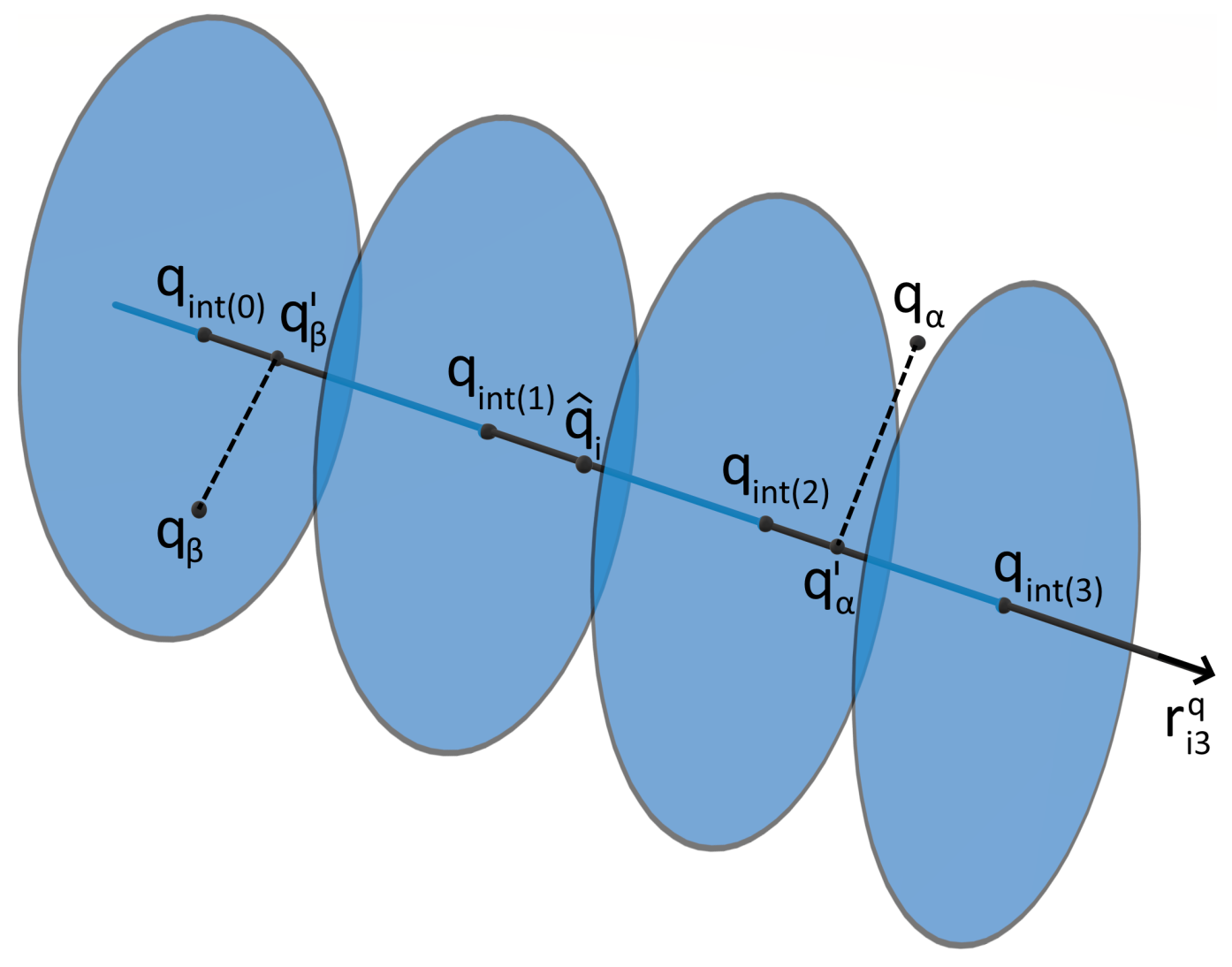
3. Direction Predictor

Standard eigendecomposition algorithms provided eigenvectors with unpredictable directions. This problem has been considered in many papers, in particular in [25,26]. The performance of the proposed $\lambda$-ICP algorithm critically depends on the quality of the eigenvector direction predictor.

Suppose that point $q_i$ in point cloud Q corresponded to point $p_i$ in P. Denote by $r_{11}^p$, $r_{12}^p$ and $r_{13}^p$ the eigenvectors of the covariance matrix in the neighborhood of $p_i$ in P, and denote by $r_{11}^q$, $r_{12}^q$ and $r_{13}^q$ the corresponding eigenvectors in Q.

Note that if the eigenvalues were placed in an ascending order, vector $r_{13}^p$ would correspond to the main inertial axis of the neighborhood, vector $r_{11}^p$ corresponding to the normal of the surface subject to the neighborhood being sufficiently flat.

The two sets of vectors define the local vector frames in P and Q.

Suppose that the directions of the vectors of the frame in Q were fixed. Our goal was to choose such directions for the vectors of the local frame in P, so that they were co-oriented with the corresponding vectors in Q.

Consider vector $r_{i3}^q$ and the mass center ${\widehat{q}}_i$ of the neighborhood in Q. Vector $r_{i3}^q$ and point ${\widehat{q}}_i$ define the oriented axis x of the local frame. Consider the orthogonal projections of all points of cloud Q to axis x.

We denoted by $q_{ent}$ and $q_{ext}$ the first and last projections on axis x. Consider the uniform subdivision of the line segment $[q_{ent};q_{ext}]$ by points $\{q_{int(0)}=q_{ent},q_{int(1)},\dots ,q_{int(m-1)},q_{int(m)}=q_{ext}\}$, where m is the number of subsegments. Figure 1 shows the described geometrical configuration. We considered each subsegment $[q_{int(j-1)};q_{int(j)}]$ and denote by $q_k^{\prime }$ the projection of point $q_i$ in Q if this projection belonged to the considered subsegment. Denote by $c_j$ the centers of subsegments $[q_{int(j-1)};q_{int(j)}]$, $j=1,\dots ,m$. We associated value $d_j$ with the subsegment in the spirit of the approach proposed in [26]:

$$d_j=\frac{1}{{\sum }_{q_i^{\prime }\in [q_{int(j-1)};q_{int(j)}]}(|c_j-q_{int(j)}|-|c_j-q_j^{\prime }|)}\sum _{q_i^{\prime }\in [q_{int(j-1)};q_{int(j)}]}(|c_j-q_{int(j)}|-|c_j-q_j^{\prime }|){|q_j-q_j^{\prime }|}^2$$

(45)

Denote by $d{s}_{i3}^q$ the following vector:

$$d{s}_{i3}^q=(d_1,\dots ,d_m).$$

(46)

We called the vector $d{s}_{i3}^q$ the descriptor of the third eigenvector in the local frame in Q. We compute the similar descriptors $d{s}_{i3}^p(+)$ and $d{s}_{i3}^p(-)$. Vector $d{s}_{i3}^p(-)$ was the inverse version of the vector $d{s}_{i3}^p(+)$.

We compared vectors $d{s}_{i3}^q$ with $d{s}_{i3}^p(+)$ and $d{s}_{i3}^q$ with $d{s}_{i3}^p(-)$ using $L_2$ norm. The smallest norm value corresponded to the direction of the third eigenvector in the local frame in P.

In a similar, way we computed the descriptors $d{s}_{i1}^q$ in Q and $d{s}_{i1}^p$ in P and vector $r_{i1}^p$. Vector $r_{i2}^p$ was the vector product $r_{i3}^p\times r_{i1}^p$.

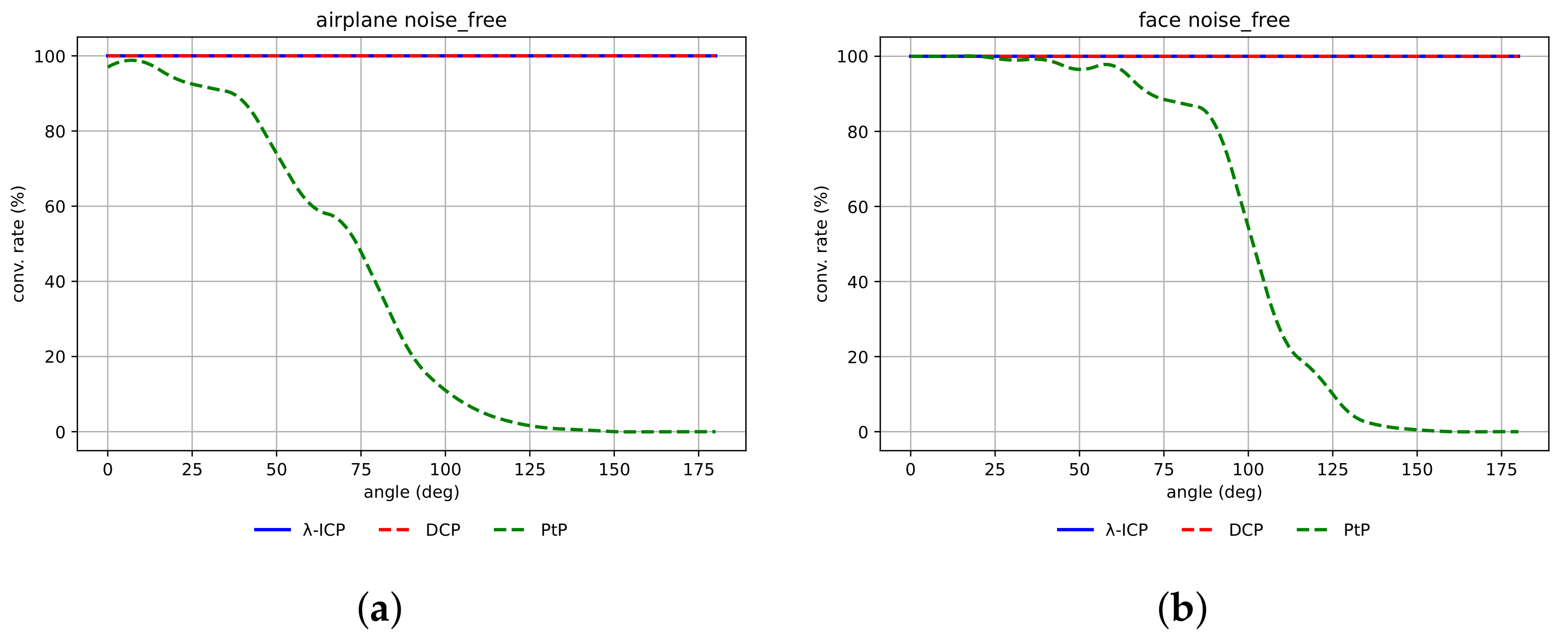
4. Computer Simulation

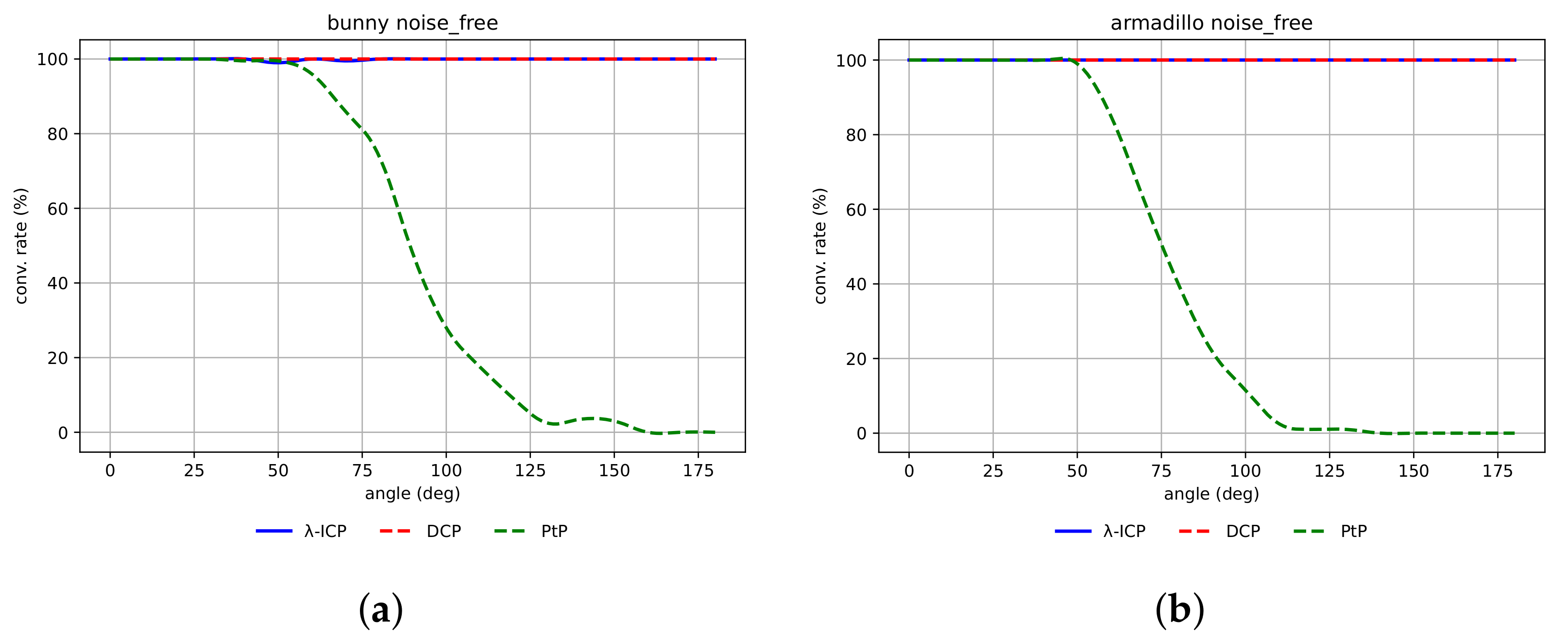
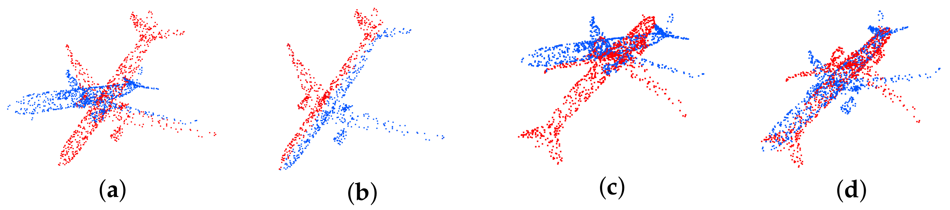
In this section, with the help of a computer simulation, we showed the performance of the proposed $\lambda$-ICP, DCP [22] and the classical point-to-point ICP (PtP) algorithms. We compared these algorithms in terms of the convergence rate (i.e., the frequency of the convergence of the ICP algorithm to a correct solution).

The algorithms $\lambda$-ICP and PtP used the standard method for searching the correspondence between clouds based on the k-d tree.

We used a trained neural network DCP [27]. Since the DCP never returned a true transformation connecting two point clouds, we only used one iteration of the DCP as a rough alignment step and after it used the standard PtP algorithm for a “polish” alignment [22].

Our experiments were organized as follows: An orthogonal geometric transformation given by a known matrix was applied to a source point cloud. The source and transformed clouds were input into a tested algorithm. The ICP algorithm converged if the reconstructed transformation matrix coincided with the original matrix with a given accuracy.

We considered two types of experiments. First, we tested the algorithms on congruent point clouds. Secondly, we tested the algorithms on a more complex problem when clouds P and Q were non-congruent. We applied additive Gaussian and impulse noise, independently, to the two point clouds to obtain non-congruent clouds.

In the case of additive Gaussian noise, each coordinate of a point was distorted by adding a Gaussian random variable with a zero-mean and a standard deviation of $\sigma =0.05$ and $\sigma =0.15$.

The considered impulse noise was defined as follows: the probability of distortion of a point by impulse noise was $0.5$; each coordinate of the distorted point was changed by adding a random variable uniformly distributed in the interval $[-0.3;0.3]$.

In the experiments, we used the four following point clouds: Stanford Bunny and Armadillo; airplane from the ModelNet40 database [22]; human face from Bosphorus database [28]. The Stanford Bunny, Armadillo and airplane clouds consist of 1024 points, the face clouds consist of 1724 points. All points lie in a centered unit sphere. Figure 2 shows the test point clouds.

The variable parameter of the DCP algorithm is the quantity of points in the considered neighborhoods. Computational experiments showed that the optimal value of this parameter for congruent clouds was 20. For noisy point clouds, for the DCP we used the maximum possible value of the parameter. The value was limited by the size of GPU memory. Our experiments were carried out on a standard desktop with Ryzen 7 1700X CPU, 32 Gb RAM, GPU NVIDIA GeForce 1080 Ti with 11 Gb GDRAM. The size of the neighborhood in the experiments with Bunny, Armadillo and airplane was 380 points; with the human face it was 220 points. In the case of the non-congruent clouds, we used a neighborhoods size of about 800–1000 points for the $\lambda$-ICP. Furthermore, $\lambda$-ICP has 21 variable $\lambda$-parameters and 1 more variable parameter equal to the number of subsegments in the direction predictor. In the experiments, we used such values of $\lambda$-parameters that ${\lambda }_{ij1}={\lambda }_{ij2}={\lambda }_{ij3}$, $j=1,\dots ,7$, $i=1,\dots ,s$.

The statistical experiments were organized as follows: We fixed the value of the rotation angle. We took a random, uniformly distributed direction vector that defined a line containing the origin of the coordinate system. This line was the axis of rotation at a fixed angle. In addition, the components of the translation vector were a random variable uniformly distributed in the interval $[0;1]$. The synthesized geometric transformation matrix (true matrix $M_{true}$) was applied to source cloud P. The tested algorithms were applied to clouds P and Q. We stated that the registration algorithm converges to true data if the reconstructed transformation matrix $M_{est}$ coincides with the original matrix with a given accuracy. To guarantee statistically correct results, 200 trials for each fixed rotation angle were carried out. The rotation angle varied from 0 to 180 degrees with a step of 10 degrees.

4.1. Congruent Case

We considered examples when a registration algorithm converges to a true transformation, and when it does not. Figure 3a shows point clouds P and Q in the initial position. Figure 3b shows P and Q in the position after registration. The estimated matrix $M_{est}$ was equal to matrix $M_{true}$. In this case, we obtained $\parallel M_{true}-M_{est}{\parallel }_F=2.44612\times {10}^{-6}$. Figure 3c shows point clouds P and Q in another initial position. Figure 3d shows P and Q in position after registration. In this case, we obtained $\parallel M_{true}-M_{est}{\parallel }_F=2.82832$.

For the congruent point clouds, we used the threshold $\parallel M_{true}-M_{est}{\parallel }_F=0.2$ as a criterion for convergence to the true transformation for all tested algorithms.

Figure 4a shows the convergence rate of the $\lambda$-ICP (blue), DCP (red) and PtP (green) algorithms for Stanford Bunny. Figure 4b shows the convergence rate for Armadillo.

Figure 5a shows the convergence rate of the $\lambda$-ICP (blue), DCP (red) and PtP (green) algorithms for the airplane. Figure 5b shows the convergence rate for the human face.

The size of the neighborhood of the DCP was equal to 20.

Table 1. Parameters of $\lambda$-ICP algorithm for the congruent case.

	Number of Subsegments	Neighborhood Size	${\mathit{\lambda }}_{\mathit{i}1\mathit{k}}$	${\mathit{\lambda }}_{\mathit{i}2\mathit{k}}$	${\mathit{\lambda }}_{\mathit{i}3\mathit{k}}$	${\mathit{\lambda }}_{\mathit{i}4\mathit{k}}$	${\mathit{\lambda }}_{\mathit{i}5\mathit{k}}$	${\mathit{\lambda }}_{\mathit{i}6\mathit{k}}$	${\mathit{\lambda }}_{\mathit{i}7\mathit{k}}$
Stanford Bunny	3	400	2	2	2	1	1	1	1
Armadillo	3	400	2	2	2	1	1	1	1
Airplane	4	1000	2	10	5	1	1	1	1
Face	3	1400	20	1	20	1	1	1	1

shows the number of subsegments of the direction predictor for $\lambda$-ICP, the size of the neighborhood and the values of parameters ${\lambda }_{ijk}$ for the point clouds, where $i=1,\dots ,s$, $j=1,\dots ,7$, $k=1,2,3$.

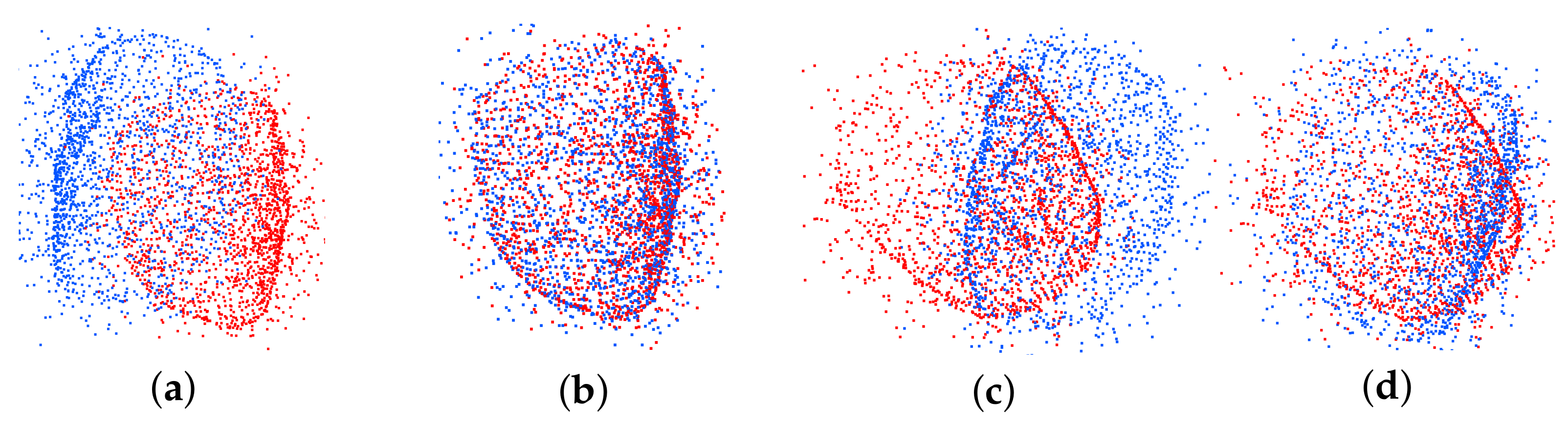
4.2. Non-Congruent Case

We considered examples when a registration algorithm converged to a true transformation for the case of non-congruent clouds, and when it did not. Figure 6a shows point clouds P and Q in the initial position. Figure 6b shows P and Q in position after registration. In this case, we obtained $\parallel M_{true}-M_{est}{\parallel }_F=0.113095$. Figure 6c shows point clouds P and Q in the another initial position. Figure 6d shows P and Q in the positions after registration. In this case, we obtained $\parallel M_{true}-M_{est}{\parallel }_F=2.56373$.

For the non-congruent point clouds, we used the threshold $\parallel M_{true}-M_{est}{\parallel }_F=0.6$ as a criterion for convergence to the true transformation for all tested algorithms.

We considered, besides the convergence rate, the RMSE based on the same experimental results.

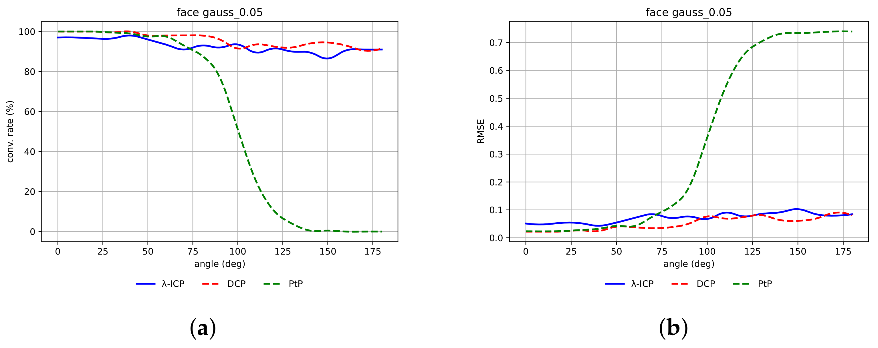
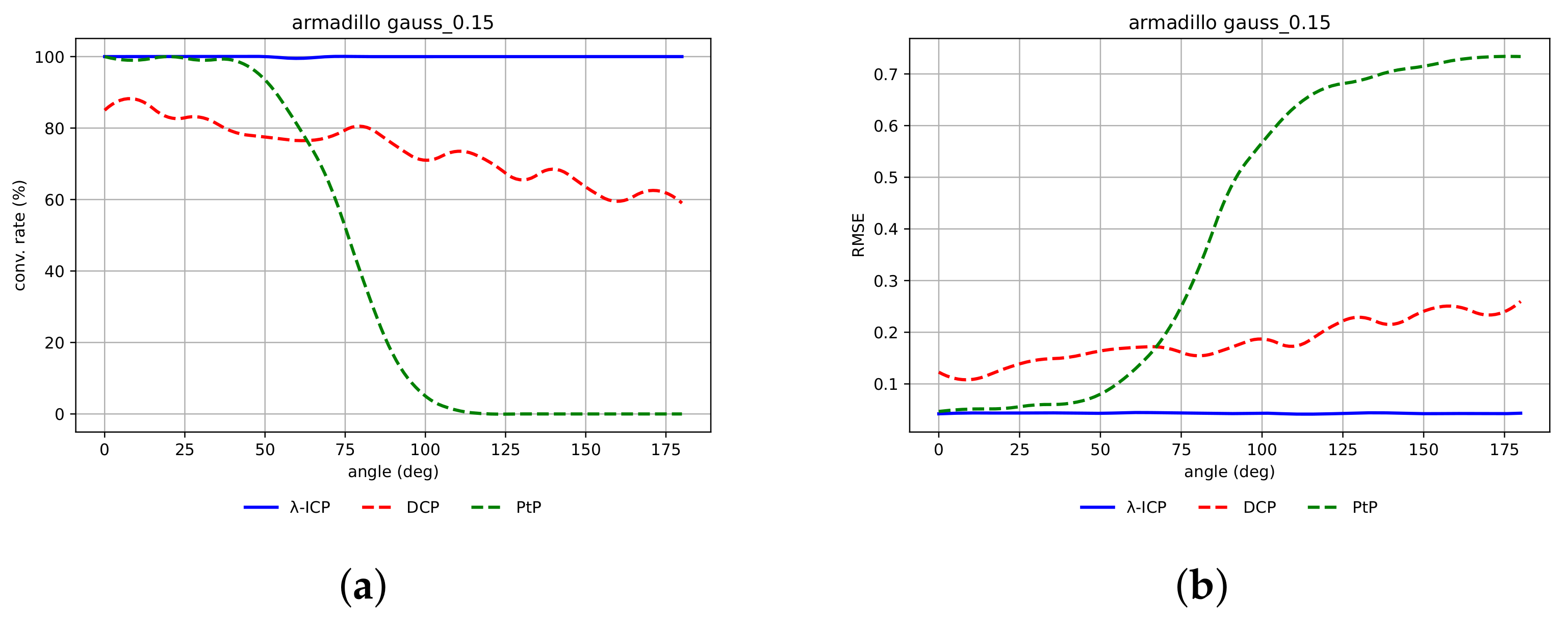
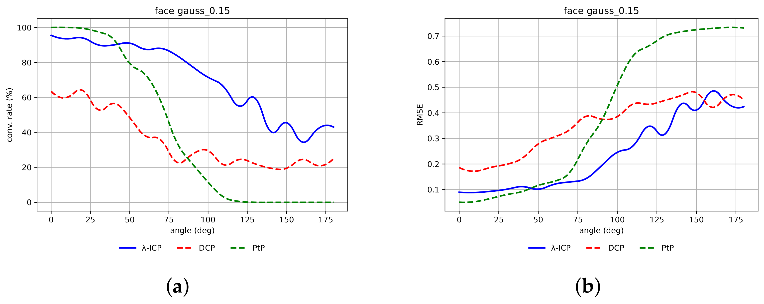
4.2.1. Gaussian Noise with $\sigma =0.05$

Figure 7 shows the point clouds distorted by Gaussian noise with $\sigma =0.05$.

Figure 8a shows the convergence rate of the $\lambda$-ICP, DCP and PtP algorithms for Stanford Bunny. Figure 8b shows the mean RMSE value computed for transformation matrices based on the same experimental results.

Figure 9a shows the convergence rate of the $\lambda$-ICP, DCP and PtP algorithms for Armadillo. Figure 9b shows the mean RMSE value computed for transformation matrices based on the same experimental results. Figure 10a shows the convergence rate of the $\lambda$-ICP, DCP and PtP algorithms for airplane. Figure 10b shows the mean RMSE value computed for transformation matrices based on the same experimental results. Figure 11a shows the convergence rate of the $\lambda$-ICP, DCP and PtP algorithms for human face. Figure 11b shows the mean RMSE value computed for transformation matrices based on the same experimental results. The size of the neighborhood of the DCP for Stanford Bunny and airplane was equal to 380, for Armadillo was 400, and for face was 220.

Table 2. Parameters of the $\lambda$-ICP algorithm for the case of Gaussian noise with $\sigma =0.05$.

	Number of Subsegments	Neighborhood Size	${\mathit{\lambda }}_{\mathit{i}1\mathit{k}}$	${\mathit{\lambda }}_{\mathit{i}2\mathit{k}}$	${\mathit{\lambda }}_{\mathit{i}3\mathit{k}}$	${\mathit{\lambda }}_{\mathit{i}4\mathit{k}}$	${\mathit{\lambda }}_{\mathit{i}5\mathit{k}}$	${\mathit{\lambda }}_{\mathit{i}6\mathit{k}}$	${\mathit{\lambda }}_{\mathit{i}7\mathit{k}}$
Stanford Bunny	3	800	2	2	2	1	1	1	1
Armadillo	3	800	2	2	2	1	1	1	1
Airplane	4	1000	2	10	5	1	1	1	1
Face	3	1400	20	1	20	1	1	1	1

shows the number of subsegments of the direction predictor for $\lambda$-ICP, the size of the neighborhood and the values of the parameters ${\lambda }_{ijk}$ for the point clouds in the case of Gaussian noise with $\sigma =0.05$, where $i=1,\dots ,s$, $j=1,\dots ,7$, $k=1,2,3$.

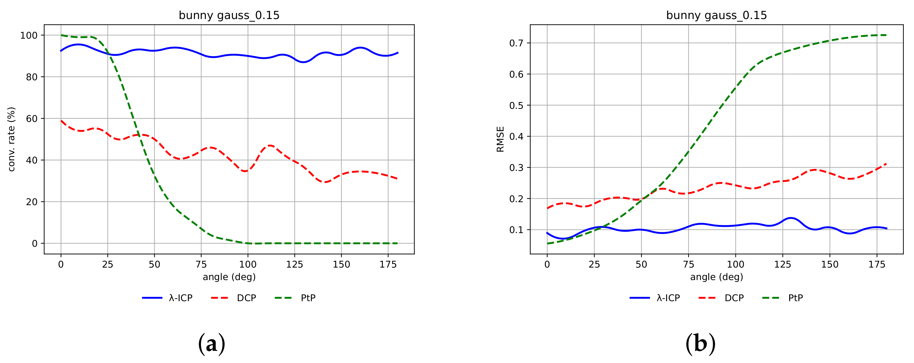
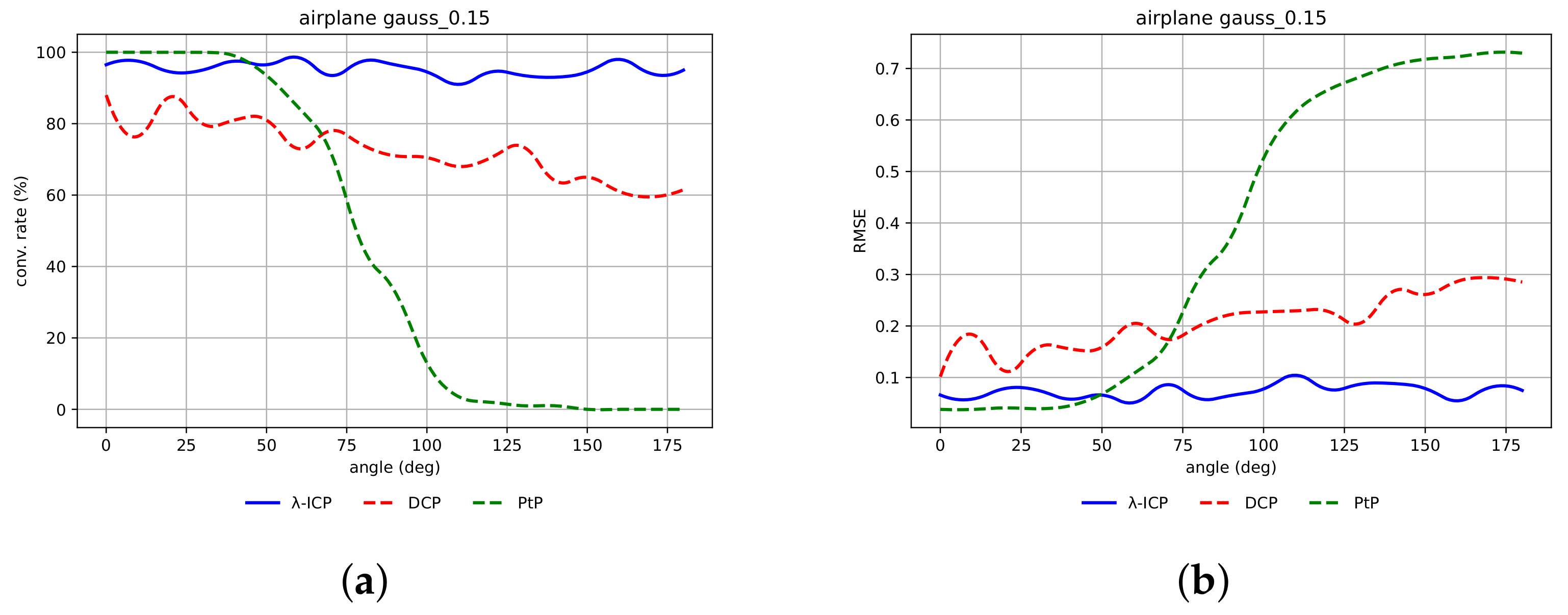
4.2.2. Gaussian Noise with $\sigma =0.15$

Figure 12 shows the considered point clouds distorted by Gaussian noise with $\sigma =0.15$.

Figure 13a shows the convergence rate of the $\lambda$-ICP, DCP and PtP algorithms for Stanford Bunny. Figure 13b shows the mean RMSE value computed for transformation matrices based on the same experimental results.

Figure 14a shows the convergence rate of the $\lambda$-ICP, DCP and PtP algorithms for Armadillo. Figure 14b shows the mean RMSE value computed for transformation matrices based on the same experimental results. Figure 15a shows the convergence rate of the $\lambda$-ICP, DCP and PtP algorithms for airplane. Figure 15b shows the mean RMSE value computed for transformation matrices based on the same experimental results. Figure 16a shows the convergence rate of the $\lambda$-ICP, DCP and PtP algorithms for human face. Figure 16b shows the mean RMSE value computed for transformation matrices based on the same experimental results. The size of the neighborhood of the DCP for Stanford Bunny and airplane was 380, for Armadillo was 400, and for face was 220.

Table 3. Parameters of the $\lambda$-ICP algorithm for the case of Gaussian noise with $\sigma =0.15$.

	Number of Subsegments	Neighborhood Size	${\mathit{\lambda }}_{\mathit{i}1\mathit{k}}$	${\mathit{\lambda }}_{\mathit{i}2\mathit{k}}$	${\mathit{\lambda }}_{\mathit{i}3\mathit{k}}$	${\mathit{\lambda }}_{\mathit{i}4\mathit{k}}$	${\mathit{\lambda }}_{\mathit{i}5\mathit{k}}$	${\mathit{\lambda }}_{\mathit{i}6\mathit{k}}$	${\mathit{\lambda }}_{\mathit{i}7\mathit{k}}$
Stanford Bunny	3	800	2	2	2	1	1	1	1
Armadillo	3	800	2	2	2	1	1	1	1
Airplane	4	1000	2	10	5	1	1	1	1
Face	3	800	20	1	20	1	1	1	1

shows the number of subsegments of the direction predictor for $\lambda$-ICP, the size of the neighborhood and the values of parameters ${\lambda }_{ijk}$ for considered point clouds in the case of Gaussian noise with $\sigma =0.15$, where $i=1,\dots ,s$, $j=1,\dots ,7$, $k=1,2,3$.

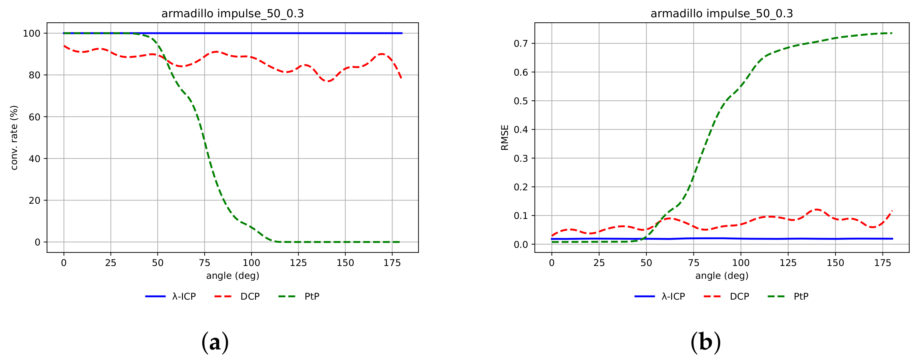
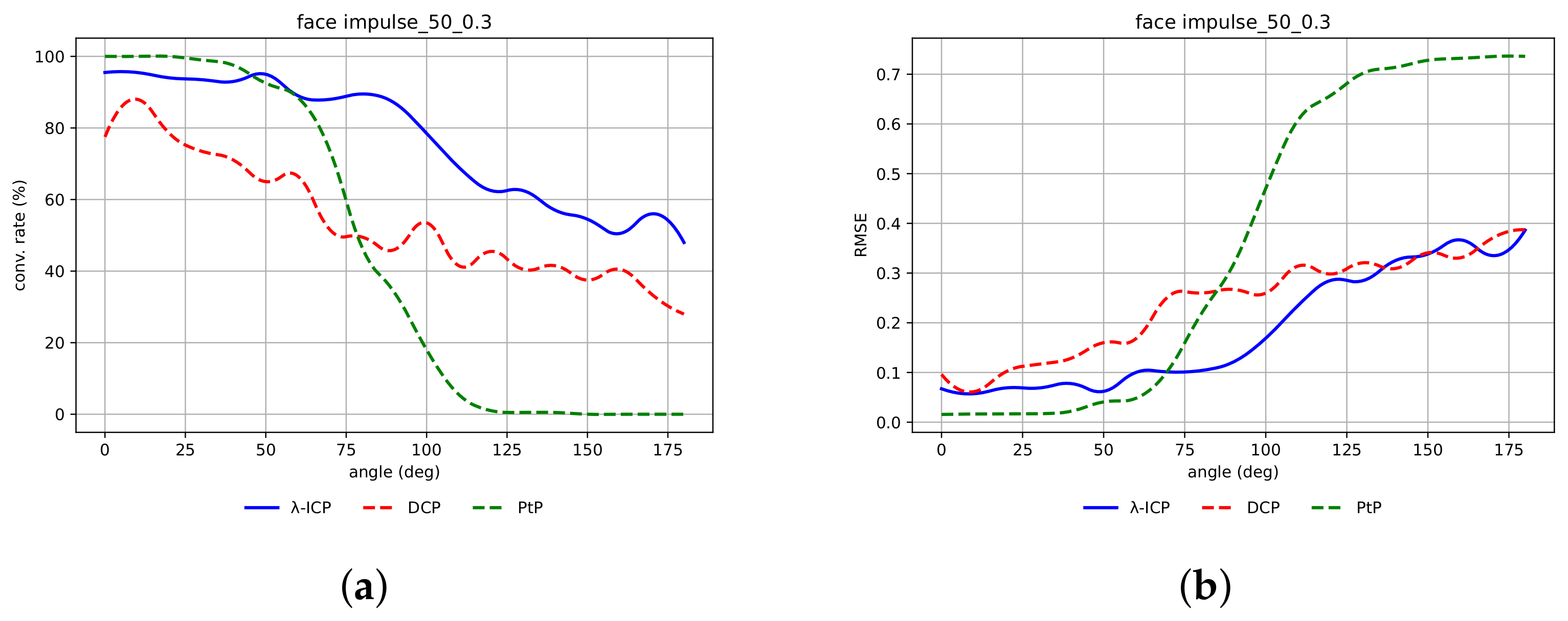
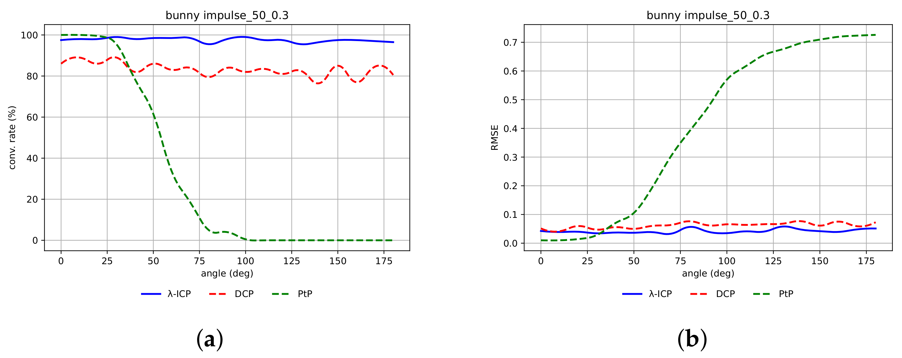
4.2.3. Impulse Noise

Figure 17 shows the tested point clouds distorted by Gaussian noise with $\sigma =0.15$.

Figure 18a shows the convergence rate of the $\lambda$-ICP, DCP and PtP algorithms for Stanford Bunny. Figure 18b shows the mean RMSE value computed for transformation matrices based on the same experimental results.

Figure 19a shows the convergence rate of the $\lambda$-ICP, DCP and PtP algorithms for Armadillo. Figure 19b shows the mean RMSE value computed for transformation matrices based on the same experimental results. Figure 20a shows the convergence rate of the $\lambda$-ICP, DCP and PtP algorithms for airplane. Figure 20b shows the mean RMSE value computed for transformation matrices based on the same experimental results. Figure 21a shows the convergence rate of the $\lambda$-ICP, DCP and PtP algorithms for human face. Figure 21b shows the mean RMSE value computed for transformation matrices based on the same experimental results. The size of the neighborhood of the DCP for Stanford Bunny and airplane was 380, for Armadillo was 400, and for face was 220.

Table 4. Parameters of the $\lambda$-ICP algorithm for the case of impulse noise.

	Number of Subsegments	Neighborhood Size	${\mathit{\lambda }}_{\mathit{i}1\mathit{k}}$	${\mathit{\lambda }}_{\mathit{i}2\mathit{k}}$	${\mathit{\lambda }}_{\mathit{i}3\mathit{k}}$	${\mathit{\lambda }}_{\mathit{i}4\mathit{k}}$	${\mathit{\lambda }}_{\mathit{i}5\mathit{k}}$	${\mathit{\lambda }}_{\mathit{i}6\mathit{k}}$	${\mathit{\lambda }}_{\mathit{i}7\mathit{k}}$
Stanford Bunny	3	800	2	2	2	1	1	1	1
Armadillo	3	800	2	2	2	1	1	1	1
Airplane	4	1000	2	10	5	1	1	1	1
Face	3	800	20	1	20	1	1	1	1

shows the number of subsegments of the direction predictor for $\lambda$-ICP, the size of the neighborhood and the values of parameters ${\lambda }_{ijk}$ for tested point clouds in the case of impulse noise, where $i=1,\dots ,s$, $j=1,\dots ,7$, $k=1,2,3$.

4.3. Summarizing the Results for Different Cases

Table 5. Average convergence rates of the $\lambda$-ICP, DCP, PtP algorithms in percent for different cases.

	Noise Free			$\mathit{\sigma }=0.05$			$\mathit{\sigma }=0.15$			Impulse Noise
	$\mathit{\lambda }$	DCP	PtP	$\mathit{\lambda }$	DCP	PtP	$\mathit{\lambda }$	DCP	PtP	$\mathit{\lambda }$	DCP	PtP
Bunny	99.9	100	50.9	98.7	99.7	45.5	91.5	42.7	26.4	98	83.2	31.4
Armadillo	100	100	43.4	100	99.1	43.8	100	73.6	42	100	86.7	41.4
Airplane	100	100	38.8	100	98.3	43.4	95.3	72.8	44.6	85.6	86.3	44.6
Face	100	100	55.5	92.8	95.8	54.9	71	35.6	40.6	76.8	54.2	45.1

shows the summarizing results of the considered algorithms. The table contains the average values of convergence rates (in percent) for the tested algorithms. Symbol “$\lambda$” in Table 5 denotes the $\lambda$-ICP algorithm.

Note that the proposed $\lambda$-ICP algorithm and DCP had a very high convergence rate for an arbitrary initial position of point clouds in $R^3$. In doing so, $\lambda$-ICP used a standard method to find the correspondence between point clouds.

5. Conclusions

In this paper, a new variant of the variational problem of the ICP algorithm was proposed. A closed-form of the exact solution for the rigid registration of point clouds based on the proposed $\lambda$-ICP algorithm and a closed-form of an approximate solution to the corresponding variational problem using a multiparameter functional were presented. We also proposed an efficient algorithm for choosing the direction for eigenvectors in point clouds. With the help of a computer simulation, the performance of the proposed algorithm was compared with that of the state-of-the-art registration algorithms. The proposed algorithm yielded a high rate of convergence to an acceptable transformation for a wide class of point clouds.

References

1. Besl, P.; McKay, N. A Method for Registration of 3-D Shapes. IEEE Trans. Pattern. Anal. Mach. Intell. 1992, 14, 239–256. [Google Scholar] [CrossRef]
2. Chen, Y.; Medioni, G. Object modelling by registration of multiple range images. Image Vis. Comput. 1992, 10, 145–155. [Google Scholar] [CrossRef]
3. Segal, A.; Haehnel, D.; Thrun, S. Generalized-ICP. Robot. Sci. Syst. 2010, 5, 161–168. [Google Scholar]
4. Serafin, J.; Grisetti, G. Using extended measurements and scene merging for efficient and robust point cloud registration. Robot. Auton. Syst. 2017, 92, 91–106. [Google Scholar] [CrossRef]
5. Makovetskii, A.; Voronin, S.; Kober, V.; Voronin, A. A regularized point cloud registration approach for orthogonal transformations. J. Glob. Optim. 2020, 1–23. [Google Scholar] [CrossRef]
6. Du, S.; Zheng, N.; Meng, G.; Yuan, Z. Affine Registration of Point Sets Using ICP and ICA. IEEE Signal Process. Lett. 2008, 15, 689–692. [Google Scholar]
7. Van der Sande, C.; Soudarissanane, S.; Khoshelham, K. Assessment of relative accuracy of AHN-2 laser scanning data using planar features. Sensors 2010, 10, 8198–8214. [Google Scholar] [CrossRef]
8. Makovetskii, A.; Voronin, S.; Kober, V.; Tihonkih, D. Affine registration of point clouds based on point-to-plane approach. Procedia Eng. 2017, 201, 322–330. [Google Scholar] [CrossRef]
9. Horn, B. Closed-Form Solution of Absolute Orientation Using Unit Quaternions. J. Opt. Soc. Am. A 1987, 4, 629–642. [Google Scholar] [CrossRef]
10. Horn, B.; Hilden, H.; Negahdaripour, S. Closed-form Solution of Absolute Orientation Using Orthonormal Matrices. J. Opt. Soc. Am. Ser. A 1988, 5, 1127–1135. [Google Scholar] [CrossRef] [Green Version]
11. Umeyama, S. Least-squares estimation of transformation parameters between two point patterns. IEEE-TPAMI 1991, 13, 376–380. [Google Scholar] [CrossRef] [Green Version]
12. Feng, Y.; Tang, J.; Su, B.; Su, Q.; Zhou, Z. Point Cloud Registration Algorithm Based on the Grey Wolf Optimizer. IEEE Access. 2020, 8, 143375–143382. [Google Scholar] [CrossRef]
13. Voronin, S.; Makovetskii, A.; Kober, V.; Voronin, A. The ICP algorithm based on stochastic approach. Proc. SPIE Appl. Digit. Image Process. XLIV 2021, 11842, 118421P. [Google Scholar]
14. Magnusson, M.; Lilienthal, A.; Duckett, T. Scan registration for autonomous mining vehicles using 3D-NDT. J. Field Robot. 2007, 24, 803–827. [Google Scholar] [CrossRef] [Green Version]
15. Newcombe, R.; Izadi, S.; Hilliges, O.; Molyneaux, D.; Kim, D.; Davison, A.; Kohli, P.; Shotton, J.; Hodges, S.; Fitzgibbon, A. KinectFusion: Realtime dense surface mapping and tracking. In Proceedings of the International Symposium on Mixed and Augmented Reality (ISMAR), Basel, Switzerland, 26–29 October 2011. [Google Scholar]
16. Shimada, S.; Golyanik, V.; Tretschk, E.; Stricker, D.; Theobalt, C. Dispvoxnets: Non-rigid point set alignment with supervised learning proxies. In Proceedings of the International Conference on 3D Vision (3DV), Quebec City, QC, Canada, 16–19 September 2019. [Google Scholar]
17. Gojcic, Z.; Zhou, C.; Wegner, J.; Wieser, A. The perfect match: 3d point cloud matching with smoothed densities. In Proceedings of the Computer Vision and Pattern Recognition (CVPR), Long Beach, CA, USA, 16–20 June 2019; pp. 5545–5554. [Google Scholar]
18. Donati, N.; Sharma, A.; Ovsjanikov, M. Deep geometric functional maps: Robust feature learning for shape correspondence. In Proceedings of the Computer Vision and Pattern Recognition (CVPR), Seattle, WA, USA, 16–18 June 2020. [Google Scholar]
19. Groß, J.; Ošep, A.; Leibe, B. Alignnet-3d: Fast point cloud registration of partially observed objects. In Proceedings of the International Conference on 3D Vision(3DV), Quebec City, QC, Canada, 16–19 September 2019; pp. 623–632. [Google Scholar]
20. Lu, W.; Wan, G.; Zhou, Y.; Fu, X.; Yuan, P.; Song, S. Deepvcp: An end-to-end deep neural network for point cloud registration. In Proceedings of the ComputerVision and Pattern Recognition (CVPR), Long Beach, CA, USA, 16–20 June 2019; pp. 12–21. [Google Scholar]
21. Wang, Y.; Solomon, J. Deep Closest Point: Learning Representations for Point Cloud Registration. arXiv 2019, arXiv:1905.03304. [Google Scholar]
22. Wu, Z.; Song, S.; Khosla, A.; Yu, F.; Zhang, L.; Tang, X.; Xiao, J. 3D Shapenets: A Deep Representation for Volumetric Shapes. CVPR 2015, 1912–1920. [Google Scholar]
23. Qi, C.R.; Su, H.; Mo, K.; Guibas, L.J. Pointnet: Deep learning on point sets for 3d classification an segmentation. In Proceedings of the CVPR, IEEE Computer Society, Boston, MA, USA, 7–12 June 2017; pp. 77–85. [Google Scholar]
24. Makovetski, A.; Voronin, S.; Kober, V.; Voronin, A. A non-iterative method for approximation of the exact solution to the point-to-plane variational problem for orthogonal transformation. Math. Methods Appl. Sci. 2018, 41, 9218–9230. [Google Scholar] [CrossRef]
25. Bro, R.; Acar, E.; Kolda, T. Resolving the sign ambiguity in the singular value decomposition. J. Chemometr. 2008, 22, 135–140. [Google Scholar] [CrossRef] [Green Version]
26. Salti, S.; Tombari, F.; Di Stefano, L. SHOT: Unique signatures of histograms for surface and texture description. Comput. Vis. Image Underst. 2014, 125, 251–264. [Google Scholar] [CrossRef]
27. Deep Closest Point. Available online: https://github.com/WangYueFt/dcp (accessed on 15 October 2021).
28. Bosphorus 3d Face Database. Available online: http://bosphorus.ee.boun.edu.tr/default.aspx (accessed on 15 October 2021).
Figure 1. Orthogonal projections of the points of cloud Q onto the axis defined by point q ^ i and vector r i 3 q .
Mathematics 09 02589 g001
Figure 2. Test clouds: (a) Stanford Bunny; (b) Armadillo; (c) airplane; (d) human face.
Mathematics 09 02589 g002
Figure 3. (a) Source cloud P (blue), target cloud Q (red) in the initial position; (b) result of alignment; (c) source cloud P (blue), target cloud Q (red) in the another initial position; (d) result of alignment.
Mathematics 09 02589 g003
Figure 4. Convergence rate of λ -ICP (blue), DCP (red), PtP (green) algorithms for: (a) Stanford Bunny; (b) Armadillo.
Mathematics 09 02589 g004
Figure 5. Convergence rate of λ -ICP (blue), DCP (red), PtP (green) algorithms for: (a) airplane; (b) human face.
Mathematics 09 02589 g005
Figure 6. (a) Source cloud P (blue), target cloud Q (red) in the initial position; (b) result of alignment; (c) source cloud P (blue), target cloud Q (red) in the other initial position; (d) result of alignment.
Mathematics 09 02589 g006
Figure 7. Point clouds with Gaussian noise, σ = 0.05 : (a) Stanford Bunny; (b) Armadillo; (c) airplane; (d) human face.
Mathematics 09 02589 g007
Figure 8. (a) Convergence rate of λ -ICP (blue), DCP (red), PtP (green) algorithms for Stanford Bunny with Gaussian noise, σ = 0.05 ; (b) mean RMSE (for transformation matrices) of λ -ICP (blue), DCP (red), PtP (green) algorithms for Stanford Bunny with Gaussian noise, σ = 0.05 .
Mathematics 09 02589 g008
Figure 9. (a) Convergence rate of λ -ICP (blue), DCP (red), PtP (green) algorithms for Armadillo with Gaussian noise, σ = 0.05 ; (b) mean RMSE (for transformation matrices) of λ -ICP (blue), DCP (red), PtP (green) algorithms for Armadillo with Gaussian noise, σ = 0.05 .
Mathematics 09 02589 g009
Figure 10. (a) Convergence rate of λ -ICP (blue), DCP (red), PtP (green) algorithms for airplane with Gaussian noise, σ = 0.05 ; (b) mean RMSE (for transformation matrices) of λ -ICP (blue), DCP (red), PtP (green) algorithms for airplane with Gaussian noise, σ = 0.05 .
Mathematics 09 02589 g010
Figure 11. (a) Convergence rate of λ -ICP (blue), DCP (red), PtP (green) algorithms for human face with Gaussian noise, σ = 0.05 ; (b) mean RMSE (for transformation matrices) of λ -ICP (blue), DCP (red), PtP (green) algorithms for human face with Gaussian noise, σ = 0.05 .
Mathematics 09 02589 g011
Figure 12. Point clouds with Gaussian noise, σ = 0.15 : (a) Stanford Bunny; (b) Armadillo; (c) airplane; (d) human face.
Mathematics 09 02589 g012
Figure 13. (a) Convergence rate of λ -ICP (blue), DCP (red), PtP (green) algorithms for Stanford Bunny with Gaussian noise, σ = 0.15 ; (b) mean RMSE (for transformation matrices) of λ -ICP (blue), DCP (red), PtP (green) algorithms for Stanford Bunny with Gaussian noise, σ = 0.15 .
Mathematics 09 02589 g013
Figure 14. (a) Convergence rate of λ -ICP (blue), DCP (red), PtP (green) algorithms for Armadillo with Gaussian noise, σ = 0.15 ; (b) mean RMSE (for transformation matrices) of λ -ICP (blue), DCP (red), PtP (green) algorithms for Armadillo with Gaussian noise, σ = 0.15 .
Mathematics 09 02589 g014
Figure 15. (a) Convergence rate of λ -ICP (blue), DCP (red), PtP (green) algorithms for airplane with Gaussian noise, σ = 0.15 ; (b) mean RMSE (for transformation matrices) of λ -ICP (blue), DCP (red), PtP (green) algorithms for airplane with Gaussian noise, σ = 0.15 .
Mathematics 09 02589 g015
Figure 16. (a) Convergence rate of λ -ICP (blue), DCP (red), PtP (green) algorithms for human face with Gaussian noise, σ = 0.15 ; (b) mean RMSE (for transformation matrices) of λ -ICP (blue), DCP (red), PtP (green) algorithms for human face with Gaussian noise, σ = 0.15 .
Mathematics 09 02589 g016
Figure 17. Point clouds with Gaussian noise, σ = 0.05 : (a) Stanford Bunny; (b) Armadillo; (c) airplane; (d) human face.
Mathematics 09 02589 g017
Figure 18. (a) Convergence rate of λ -ICP (blue), DCP (red), PtP (green) algorithms for Stanford Bunny with impulse noise; (b) mean RMSE (for transformation matrices) of λ -ICP (blue), DCP (red), PtP (green) algorithms for Stanford Bunny with impulse noise.
Mathematics 09 02589 g018
Figure 19. (a) Convergence rate of λ -ICP (blue), DCP (red), PtP (green) algorithms for Armadillo with impulse noise; (b) mean RMSE (for transformation matrices) of λ -ICP (blue), DCP (red), PtP (green) algorithms for Armadillo with impulse noise.
Mathematics 09 02589 g019
Figure 20. (a) Convergence rate of λ -ICP (blue), DCP (red), PtP (green) algorithms for airplane with impulse noise; (b) mean RMSE (for transformation matrices) of λ -ICP (blue), DCP (red), PtP (green) algorithms for airplane with impulse noise.
Mathematics 09 02589 g020
Figure 21. (a) Convergence rate of λ -ICP (blue), DCP (red), PtP (green) algorithms for human face with impulse noise; (b) mean RMSE (for transformation matrices) of λ -ICP (blue), DCP (red), PtP (green) algorithms for human face withi mpulse noise.
Mathematics 09 02589 g021