Abstract
Information on the correlations from solar Shack–Hartmann wavefront sensors is usually used for reconstruction algorithms. However, modern applications of artificial neural networks as adaptive optics reconstruction algorithms allow the use of the full image as an input to the system intended for estimating a correction, avoiding approximations and a loss of information, and obtaining numerical values of those correlations. Although studied for night-time adaptive optics, the solar scenario implies more complexity due to the resolution of the solar images potentially taken. Fully convolutional neural networks were the technique chosen in this research to address this problem. In this work, wavefront phase recovery for adaptive optics correction is addressed, comparing networks that use images from the sensor or images from the correlations as inputs. As a result, this research shows improvements in performance for phase recovery with the image-to-phase approach. For recovering the turbulence of high-altitude layers, up to 93% similarity is reached.
1. Introduction
Artificial intelligence methods have led to major improvement in several fields of the science of engineering [1]. As a mathematical tool to perform numerical approximations, they are broadly used to represent complex physical systems, whose analytical models are way too complex to work with, or even improve other numerical approaches both in terms of time consumption and performance. Among the broad range of techniques considered as artificial intelligence, some of them are used satisfactorily as a solution to cutting-edge problems, such as deterministic artificial intelligence [2], which implies an alternative to stochastic methods [3]. Other options include neural networks, since the variety of architectures of neural networks allows for managing different types of problems, from those that require a numerical approximation as a regression problem to those that are classification problems.
The flexibility of the networks not only relates to what they are expected to obtain but also the manner of the information of the problem being measured. Thus, several types of information may be used to work with neural networks; data vectors are for the simplest models of networks, but two-dimensional arrays, such as images, or even higher dimensional tensors can be used to feed a network.
Artificial neural networks, as learning algorithms [4], considered under a supervised learning process will have their answers verified against true information measurements, usually real data or simulated data, and then adjust their inner parameters to better fit the problem by means of an optimization algorithm. As a consequence, a network can be considered a malleable model that fits a given problem by solving a multidimensional optimization problem.
While this seems to be a clear advantage, the search for local minima, given a particular architecture, does not have a perfect answer when expecting models to work toward real-time computation. Moreover, this issue becomes larger when considering all the possible hyperparameters that tune the topology and architecture of a neural network. These different approaches to the solution of a problem make it difficult to choose an answer. In particular, the application of neural networks considered in this work for adaptive optics (AO) has the same issue.
In general, AO is a set of techniques related to astronomical telescope imaging, where atmospheric distortions modify the images taken by those telescopes. This is due to the changing nature of the atmosphere, whose turbulences are usually modeled by statistically based models such as those of Von Karman [5] or Kolmogorov [6,7]. Adaptive optics includes a set of techniques and elements that allow for correcting the turbulent effects, from sensing the turbulences with wavefront sensors to correction of the wavefront of the image in deformable mirrors and other processes, such as estimation of the turbulent effects with a reconstruction algorithm.
In recent years, the latest issue is one that has been broadly studied with the application of artificial neural networks [8]. As it was previously mentioned, it is not easy to select an adequate network, and thus this problem was one of the main issues addressed in previous works [9]. An attempt for an answer in the case of nocturnal AO has been deliberated in previous papers, yet a study for the solar situation is necessary [10,11]. Although in previous works, some networks such as multilayer perceptrons (MLPs) and convolutional neural networks (CNNs) were checked [12,13], this work presents improvements through the use of fully convolutional networks (FCNs), comparing the differences between using solar correlations as inputs for the networks and the full image from the solar Shack–Hartmann (SH) wavefront sensors.
This paper is organized as follows. Section 2 includes the artificial intelligence methods described above, as well as some insights about solar adaptive optics modeling and details about the simulation platform. Section 3 shows the results of the selected topologies for the two cases considered, and Section 4 includes a detailed discussion about the obtained results. Finally, in Section 5, our conclusions are put forward.
2. Materials and Methods
2.1. Artificial Inteligence
Artificial intelligence methods have become, in recent times, fundamental in daily applications for both scientific and engineering purposes. Their key feature is their capability to learn, supervised or unsupervised, from a great amount of data and extract patterns to provide a response to a problem [14]. In this research, artificial intelligence was used as the reconstruction system of a solar AO system, based on the results and previous performance proven for nocturnal AO. For these purposes, artificial neural networks (ANNs) were used. Choosing one type of architecture or another highly depends on the problem to be solved. Usually, multilayer perceptrons (MLPs) are used to process vectorial inputs, or low-dimensional tensors that can be easily vectorized [15]. Convolutional neural networks (CNNs) rely on the use of kernels or filters that are trained to extract and process the most relevant features from an image-like input, as well as for tensor inputs [16]. They usually have a segment where the data are resized to be smaller while maintaining the information, allowing one to vectorize the data and add an MLP segment at the end of the network. Other alternatives include fully convolutional networks (FCNs) [17], which take the full input, and after processing the main characteristics, the deconvolutional layers are set to recover from the characteristics in the shape of a tensor.
In this work, FCNs were tested for phase reconstruction. The ANNs were used with wavefront sensor images of the frames of the Sun and with correlations, in order to check the input data that best fit with the FCNs’ performance.
2.1.1. MLPs and Backpropagation
A multilayer perceptron is based in the computation of responses of individual computation units of neurons, which are sorted in layers; each of them computes the following calculus [18]:
where for each neuron , the input values from are weighted by the values , and then a bias is added. All these computations are then modified by an activation function . The outputs are those defined as .
The activation functions work as a normalizing modification of the output, usually a hyperbolic tangent or sigmoid, whose images are restricted to and , respectively [19]. Other activation functions that are commonly used are rectified linear unit (ReLU), parametric linear unit (PReLU), etc. [20].
Neurons are assigned to layers, which are sorted so all the neurons of each layer can be densely connected to all the neurons of the following layer, which is conducted by means of assigning the weights to those connections. Once the last layer gives an output, it is considered as the output of the network to the inputs given.
At first, the network’s weights are set as random (thus, sometimes, they are set following some rules, as some predefined filters); consequently, the network’s response to an input would be random, meaning the model must be trained. To estimate the differences between the obtained output and the desired value, a loss function is applied. Usually, measures such as mean squared error (MSE) or RMSE (root mean square error) are applied for regression problems. Cross-correlation is often used for classification purposes [21].
The backpropagation algorithm is set to change the values of the weights according to the information obtained from the loss function over a training set [22,23]. This is then a multivariate optimization problem over the weights as variables, whose dimension depends explicitly on the size of the network. The simplest way to approach this problem is to set a stochastic gradient descent algorithm [24], where for each iteration of the samples from the training set, the weights are updated as follows:
where is the loss function, and its partial derivative is computed to upgrade the weight values in the direction of the negative gradient. The parameter is called the learning rate and is used to regulate the magnitude of the steps taken in the direction of the negative gradient.
Other optimizers include the momentum of inertia or several modifications, such as Nesterov (Adam), Adagrad, and Adadelta, to improve the convergence of the method towards local minima [25].
2.1.2. Convolutional Neural Networks
For multidimensional inputs, such as those matrixes that represent images, or tensors, vectorization to apply an MLP may not be adequate. In these situations, convolutional layers are used to process the full input, by using kernels or filters [26]. These are set in the convolutional layer, obtaining a map of characteristics from each kernel applied, which is applied by a discrete convolution, given by
for an image and a kernel , over , the sizes of the kernel as a matrix, as well as the matrix . At first, the values of are set as random or as predefined filter values but, over iterations, are intended to be minimized with the same procedure explained for the MLPs, taken as an optimization problem.
Convolution layers also include the application of an activation function. At first glance, characteristic maps maintain the size of the original matrix for each of the characteristic maps, so in order to downsize the data, usually max-pooling is applied [16].
After the desired number of convolutional layers, the processed data are vectorized to be the input of an MLP section.
2.1.3. Fully Convolutional Neural Networks
However, if the desired output should be a multidimensional array, other options can be considered. The topology of an FCN allows having these outputs, particularly after the succession of convolutional layers, a section of deconvolutional layers whose calculus consists of the transpose of discrete convolutions over the correspondent kernels or convolution window.
In FCNs, the classification block presented at the end of a common CNN is substituted by the deconvolutional block, allowing the ANN to obtain a new image as output from the several maps of characteristics extracted from the input by the convolutional block; an example of an FCN topology is shown in Figure 1. Its performance consists of a new extended image from small images with the main features of the inputs. Therefore, for this type of ANN, the principal block of the ANN is the convolutional one as in the previous case.
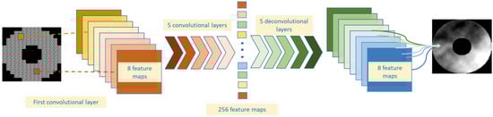
Figure 1.
Schematic representation of the FCN used throughout this research. The comparison is made in both cases with the same FCN topology.
One of the main features of FCNs is not just plain processing downsizing through convolutions and then recreating bigger matrixes through deconvolutions, it is the design where features from the convolutional section are then fused into the adequate parts of the deconvolutional section. Thus, this allows passing spatial information deeper to sections where it may have been lost.
FCN is the ANN topology used for this research, as both the input and the output data used for the comparison consist of images. As input data, the image of the wavefront received by the Shack–Hartmann wavefront sensor or the image of the calculated cross-correlations for several moments is given, being the profile of the turbulence phase for each moment of the desired output.
2.2. Solar Adaptive Optics
Adaptive optics is the branch of astronomy that corrects and improves the quality of images taken by telescopes. Due to the fluid nature of the atmosphere, the refractive index varies rapidly, meaning any light that passes through it has its wavefront displaced due to the change in velocity of the photons when passing through the different refractive indexes [27].
Kolmogorov models are some of the most used models to model atmospheric turbulences. They are based in the layers of the turbulence, characterizing it through the heights of the layers, their relative forces, winds, the energy generated by external-scale processes that influence and cause phenomena on smaller scales , large-scale air movements , and Fried’s coherence parameter , which generalizes some of the properties that include aspects such as composition and temperature. The Kolmogorov spectra are given by
where is the refractive index structure constant.
Fried’s coherence length ( represents a very useful parameter in astronomy terms as it contains information about the turbulence intensity, the wavelength, and the propagation path for an incoming wavefront. It is defined as follows:
where represents the zenith angle.
The value can be defined as the diameter of a pupil where the RMS wavefront aberration value is 1 radian, and it is expressed in length terms, commonly in cm. This means that the lower the value, the more intense the aberrations. To put this in context, a common astronomical observation day would be represented by an value higher than 16 cm. If the value is lower than 12 cm, astronomical observations are usually postponed, due to bad turbulence conditions. values less than or equal to 8 cm correspond to extremely bad atmospheric turbulence, as it could be a stormy day.
To correct those aberrations, mechanical systems to refract the beams of light at the adequate wavelengths return the images to their original shape. Usually, the distortions are measured by Shack–Hartmann wavefront sensors (SHWFSs). In night-time observations, SHWFSs consist of an array of convergent lenses, consequently having as many estimates of the turbulent profile of the atmosphere as lenses in the sensor; as each lens causes the light to converge, the estimation, which is a blurred concentrated spot of light, whose gravity center is called a centroid, corresponds to the deviation from the center of the CCD sensor.
Then, typically a system of AO has some SHWFSs that measure the distortions and a deformable mirror that reflects the adequate wavefront, and they need a reconstruction algorithm that estimates the turbulent profile. For these algorithms, the most traditional approach is least squares (LS), but AI alternatives have been proven successful approaches [28].
For solar observations, however, the situation differs in several ways: First, the energy received by the atmosphere from the Sun directly disturbs the atmosphere, having more turbulent layers as a result of the excess of energy. The reconstruction must take this into account, since one point in time may be completely different to the next, while in night observation, variations are slower as the turbulence is stabler. From all of the turbulent profile, most of the variations occur in the ground layer, also due to the heat radiated by the Earth and the telescope’s pupil during daylight hours.
Another major issue, which changes the way of measuring the profile, is the fact that the Sun’s proximity to Earth implies that it cannot be considered a point source. Wavefront measurement should be conducted without guide stars. The estimation cannot be carried out, then, with centroids, as the SHWFS receives on each subaperture an extended image, being necessary to calculate the correlations between the images that appear in the subapertures, in order to estimate the variations in the turbulent profiles. An example is shown in Figure 2.
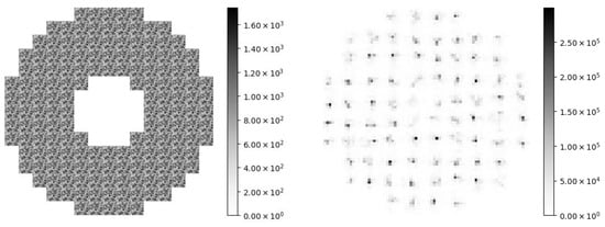
Figure 2.
Information received by the SHWFS in diurnal observation on the left and in night-time observations on the right. In solar observations, due to the source’s proximity, an extended image is received by each subaperture of the SHWFS, saturating all the pixels instead of blurred spots as happens in the night scenario, meaning that the algorithms used in night AO have to be modified in diurnal AO.
The way to calculate the correlations is by using an image from one subaperture as the reference image at the beginning of the observation; thus, the variations detected by sensors are measured by the comparisons with the reference image. From the first images, any can be used as the reference one, but commonly, one of the brightest images should be chosen. A cross-correlation between the “live” image, measurement from the sensor at each individual instant, and the reference image is estimated according to the following [29]:
where is the live image and is the reference image obtained from the SH, where x denotes the spatial coordinate in the lower contour of the sensor and Δ denotes a spatial lag, the result of obtaining the image at a different subaperture.
The actual calculation of the covariance can be conducted by a Fourier transform given by
where , are direct and inverse Fourier transforms, respectively. stands for the complex conjugate of a Fourier transform [30]. Results of correlated images from a solar SH are exemplified in Figure 3.
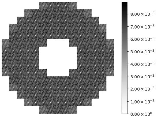
Figure 3.
Image of the cross-correlations calculated by the SHWFS from a randomly chosen sample of the training dataset. A spot is situated approximately in the center of each subaperture that corresponds to the maximum of the CC.
The position of the maximum of the cross-correlation CC is a linear measure of the displacement between the reference image and the given subaperture; therefore, the aberration of the wavefront will already be identified, even more so when the gradients or inclinations are measured, which will be carried out in the same way as conducted in night adaptive optics from the centroids of each subaperture. Once the values of the coefficients are known, the received wavefront has already been reconstructed, meaning the next step that will be carried out will be to obtain the values of the positions that each DM must occupy to correct the aberration suffered.
2.3. Durham Adaptive Optics Simulation Platform (DASP)
The DASP consists of a simulation platform developed by Durham University for night and solar observations [31]. The software allows the user to determine the parameters of the simulation; several AO configurations can be implemented such as SCAO, MCAO, and MOAO. Moreover, in the simulations, the number of components can be selected by the user, such as the number of SHWFSs and the number of DMs. The features of each component can also be chosen, such as the telescope diameter, the number of subapertures of the SHWFS and its number of pixels, or the number of actuators of the DM. Due to the quality of the simulations carried out by the DASP, the platform is currently used in simulations for forthcoming real instruments, such as the Extreme Large Telescope (ELT) or the 12 m Chinese Large Optical Telescope [31].
The DASP simulates the atmospheric turbulence according to Kolmogorov’s model, which is implemented by Monte Carlo simulations. Some parameters of this model can be chosen by the user, such as the r0 value that determines the intensity of the whole turbulence, as well as the number of turbulence layers, the weight of each one over all of the turbulence, their height, and their wind direction and velocity.
A very interesting feature of this platform is that multiple pieces of information of the intermediate processes of the AO system can be saved, allowing for comparisons of the research. For each situation, the information received by the SHWFS, the cross-correlations calculated by the SHWFS (in solar observations), the slope measurements on each subaperture, the turbulence phase, Zernike’s coefficients of the turbulence phase, or the voltage for the DM’s actuators can be extracted from the software.
For this research, the DASP was used as the tool to generate the datasets needed to train, validate, and test the ANN models. Simulations were conducted according to the parameters shown in the next section, saving the image of the wavefront received by the SHWFS and its corresponding correlations, which are the input of the ANN models. The phase profile for each moment was also saved, being the desired output of our AI reconstruction system. Thus, the dataset to train and test both models was utilized in all simulations to make a realistic comparison.
2.4. Experimental Setup
The training of the networks, as well as the simulations, was performed on a computer running on a Ubuntu LTS 18.04.4, with an Intel Xeon CPU W-3235 @3.3Ghz, 512 Gb DDR4 memory, Nvidia GeForce RTX 2080 Ti, and SSD hard drive. Python was the computer language used, along with TensorFlow and Keras. The Gregor Solar Telescope [32] configuration was replicated in the simulations, with a 1.5 m pupil diameter, working in a Solar SCAO configuration. As the objective is to compare the behavior of the FCNs depending on the input data, all the simulations were conducted over the same region of the Sun.
The training dataset consisted of 80,000 simulated images of the information received by the SHWFS and the calculated correlations with their corresponding profile of the turbulence phase, which is the desired output of both FCN models. All the simulations related to two turbulence layers, the first one being situated at 0 m height with a weight of 10% of the turbulence, and the second one being another turbulent layer whose height varied from 1 to 20,000 m in steps of 100 m each for the remaining 90%. The r0 values of the turbulence varied from those corresponding to extremely turbulent scenarios to values from a calm observation day. In numerical terms, they range from 8 to 16 cm of r0 in steps of a cm. For each situation, 50 consecutive simulations were conducted, resulting in a total of 80,000 simulations. To validate the models during the learning process, a test dataset was constructed with 3000 situations where both the height and the r0 value varied between the same terms, but in higher steps.
The ANN models were tested with 12 additional test datasets that consisted of randomly generated turbulence phases unknown to the networks. Each dataset corresponded to a fixed r0 value from 7 to 19 cm and a determinate range of the height for the atmospheric turbulence. One half consisted of turbulence between 0 and 3000 m that represents the ground layer, and the other half between 9000 and 12,000 m. The datasets allowed analyzing the performance of the FCNs with several turbulence situations and comparing which input data fit better according to the situation. Each dataset was composed of 600 samples.
The ANNs’ performance was analyzed by visual comparison and analytical error. For the second case, the residual wavefront error (WFE) was employed:
where represents the turbulence phase’s pixels of the FCN’s output and is those of the desired output. This error can also be measured in percentage by dividing (8) by the RMSE WFE of the simulated profile phase.
Selected FCN Topology
To make a realistic comparison, the same network topology was employed for both types of input data considered. The topology consisted of a convolutional block with 6 convolutional layers, where the input shape of the image of 360 × 360 was reduced, applying strides of sizes 1, 2, or 3 pixels in both directions, to 256 feature maps of size 5 × 5. They were passed to a deconvolutional block formed by 6 deconvolutional layers that, with the same size of strides as those from the previous block, obtained, as final output, an image of size 90 × 90 pixels, as the simulated turbulence’s phase. Padding was added in all the layers, and the ANN was trained with Nesterov’s gradient descent optimization algorithm, with a 0.02 learning rate and a momentum value of 0.7. All the layers applied the same activation function, the hyperbolic tangent. A schematic representation of the selected FCN can be seen in Figure 1.
3. Results
This section presents two different scenarios showing the performance of the FCN when comparing the two types of input images in scenarios of low-height turbulences, trying to replicate the ground layer, in one subsection, and high-height turbulences in the other.
The data shown in the next table correspond to the mean of the residual WFE of the reconstruction, the mean WFE residual of the phase’s profile over the 600 samples of each test, and the mean value of the similarity of the reconstructions. The similarity is calculated as the mean value of the quotient of the RMSE WFE of the reconstruction between the simulated one for each sample.
The recall time needed per sample by the FCN to reconstruct the turbulence’s profile is also shown.
3.1. Ground Layer Turbulences
The errors committed in the reconstruction of ground layer turbulences by the FCNs are shown in Table 1. All the test datasets consist of 600 images of ground layers between 0 m and 3 km of height; therefore, the results given consist of the mean value over all the samples of the test. Then, several figures of randomly chosen samples of each test dataset are shown for a visual comparison.

Table 1.
Results obtained for the ground layer reconstructions. WFE net refers to the RMSE WFE calculated over the images given by each FCN as output, while WFE residual refers to the RMSE WFE of the image that is obtained as the difference between the output of one ANN and the original simulated image. Both terms are measured in radians (rad). SHWFS refers to the ANN that uses as input the information received by the subapertures of the sensor, while CC refers to the ANN that uses the cross-correlations (CC) as inputs. The time column shows the mean time over the dataset per sample for each ANN, measured in milliseconds (ms).
In Figure 4, several examples of the reconstructions carried out by both FCNs with their corresponding original image are shown for a visual comparison. There is an example for each used test dataset.
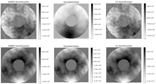
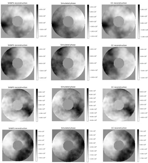
Figure 4.
Comparison of the reconstructed phases for ground layer turbulences with the original one. Each row corresponds to an example of a sample of each test dataset used with values from 7 to 17 cm in steps of 2 cm and its corresponding reconstructions. On the left, the reconstructions carried out by the FCN whose inputs are directly the information received by the SHWFS are shown. In the center of the image, the original turbulence phase simulated is shown, while on the right, the reconstructions carried out from the cross-correlations are shown.
3.2. High-Altitude Layer Turbulence
In this subsection, the results of the reconstruction for high-altitude layers applied over simulations with turbulent profiles of altitudes between 9 and 12 km in height are shown. The results are presented in the same way as in the previous subsection: first, Table 2 shows the analytical values of the errors, similarity, and time needed per reconstruction, and then Figure 5 allows for a visual comparison of a randomly selected example from each test dataset.
Table 2.
Results obtained for the high-altitude layer reconstructions. WFE net refers to the RMSE WFE calculated over the images given by each FCN as output, while WFE residual refers to the RMSE WFE of the image that is obtained as the difference between the output of one ANN and the original simulated image. Both terms are measured in radians (rad). SHWFS refers to the ANN that uses as input the information received by the subapertures of the sensor, while CC refers to the ANN that uses the cross-correlations (CC) as inputs. The time column shows the mean time over the dataset per sample for each ANN, measured in milliseconds (ms).
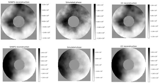
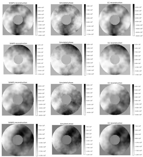
Figure 5.
Comparison of the reconstructed phases for high-altitude layer turbulences with the original one. Each row corresponds to an example of a sample of each test dataset used, with values from 7 to 17 cm in steps of 2 cm, and its corresponding reconstructions. The images are placed following the order presented in Figure 4.
4. Discussion
The performances of two different approaches to recover the turbulent profile’s phase in the context of solar AO were presented in this research. Information received by the SHWFS or its calculated cross-correlations was used as input data for an FCN. The main objective is to know if the loss of information due to pre-processing the information received affects the quality of the reconstruction of a reconstruction system, particularly when using an ANN.
Both methods were analyzed in terms of the computational time needed by the RS, where a visual representation of the obtained results is shown in Figure 6. The figure depicts how the use of cross-correlations minimally decreases the time needed per sample by the RS independently of the type of turbulence layer reconstructed. The time is reduced, in mean terms, by approximately 3% for the ground layer and 4% for the second case, being irrelevant values for the selection of the best model. Moreover, considering the case of cross-correlations, the recall time needed was not considered, meaning the method would be slower than the one with SH images.
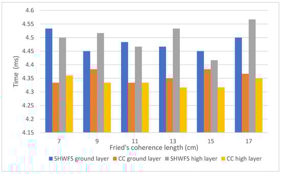
Figure 6.
Required time needed per epoch for both models in the two cases of turbulence profiles considered. SHWFS represents the FCNs whose inputs are directly the information received by the wavefront sensor, while CC reconstruction corresponds to the cross-correlations. To make comprehension easier, the bars for each case are in the same order as the legend.
The quality of the reconstruction was analyzed in analytical terms of the WFE and similarity, and a visual comparison could be also made, as shown in Figure 4 and Figure 5.
In both methods, it is observed that the ground layer is more difficult to reconstruct given the low values of similarity of the turbulence’s phases. This matches with the initial assumption as ground layers have always been a big challenge for AO systems, especially in solar observations. As it has been mentioned in Section 2, in diurnal observations, due to the impact of the solar energy reflected by the Earth, ground layers have more energy and faster variations. This is reflected in Figure 7 and Figure 8, where a clear trend is seen when comparing the results for ground layer turbulences and altitude layer turbulence for both methods. In the case of the SHWFS neural networks, the residual WFE committed is, in mean terms, for the six tests, 34% lower when the turbulence layer is situated at high altitudes, while in the CC reconstruction, that value is 39%. The height of the turbulence has more influence in the reconstruction when all the information received by the Shack–Hartmann sensor is used as the input of the neural network. This fact can be expected since cross-correlations are processed data that usually have approximately the same aspect, being robust to variations in the turbulence, which does not happen in the case of the light received by the sensor. These variations affect the response of the ANN and affect the quality in the reconstructions, which strongly depends on each scenario, in contrast with the CC FCN case.
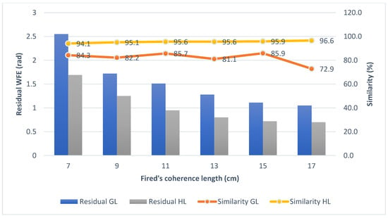
Figure 7.
Influence of the height in the reconstructions, using the information received by the sensor as inputs for the FCN for the several values tested. To make comprehension easier, the bars for each case are in the same order as the legend and each case has its own markers.
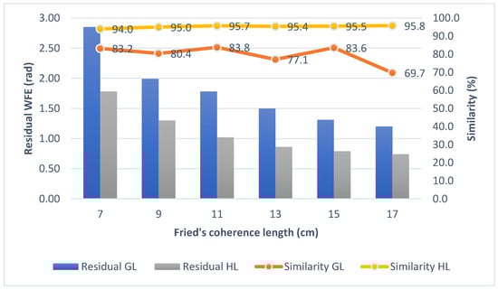
Figure 8.
Influence of the height of the layers (ground layers (GL) and high-altitude layers (HL)) in the reconstructions carried out using the cross-correlations as inputs for the FCN for the several values tested. To make comprehension easier, the bars for each case are in the same order as the legend and each case has its own markers.
The same analysis can be conducted when considering the influence of the value in the quality of the reconstructions. The error committed lowers as the value increases for both cases, something expected as the intensity of the turbulence also decreases. However, the difference in the error committed for an value compared with the previous one is slightly smaller in the case of the CC network. For the first case, for example, between 7 and 9 cm, in the SHWFS case, the error is 33% lower for 9 cm, as in the CC case, where it is 30%. Thus, the CC FCN appears to be more robust to turbulence variations than the SHWFS one, since the second one receives much more information of the turbulence for each moment.
The results explained can visually be analyzed in Figure 4 and Figure 5. The profiles of the turbulence phases reconstructed in Figure 4 have less definition than the Figure 5 ones, as they correspond to ground layer turbulence. Moreover, as the rows of the figures are analyzed, the definition is clearly higher in the rows below (higher situations) than in those above.
Finally, we present the comparison of the results obtained for both methods, using the light received by the Shack–Hartmann sensor as input (SHWFS method) or the cross-correlations (CC method). In Figure 9, the representation of the similarity obtained by each method in the reconstructed turbulence phases for all the situations tested can be seen. The results are very similar in both methods, but a clear trend can be seen; for every case, the reconstruction carried out using all the information received by the Shack–Hartmann sensor improves the similarity to the one carried out from the cross-correlations. Nevertheless, that difference is more accentuated for the cases of ground layer turbulences than for the other ones. The loss of information in the process of establishing cross-correlations between the subapertures means the ANN is not able to reconstruct the turbulence phase in such a similar way. For the cases of ground layer reconstructions, the SHWFS method obtains increases in the similarity between 1.1% and 4%, being the mean for the six tests, obtaining an average improvement of 2.7% in similarity terms. That difference is lower for the high-altitude layer reconstruction, the average being only 0.25%.
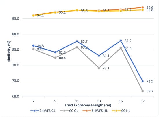
Figure 9.
Comparison of the similarity obtained by both methods for ground layer (GL) and high-altitude layer (HL) situations. Note that the markers in the figure are fixed for each ANN model.
In order to analyze the quality of the results obtained by both ANN models, some data of other AO reconstructors used in previous research [33] are compared. In Table 3, the residual WFE obtained in reconstructions applying the least squares method (LS) [10], the most commonly used algorithm in real AO systems, is shown. The characteristic of the AO system is the same as in this research in terms of the telescope’s pupil diameter and subapertures. The data given are calculated as an average for turbulence layers from 0 to 16 km in height over 400 samples; therefore, in this case, there are no specific reconstruction error values for ground layer or high-altitude layer reconstructions. Comparing the residual WFEs of Table 3 with the ones obtained for the high-altitude layer reconstructions using a polynomial approximation of order 3, both methods based on FCNs provide lower WFEs. The FCN obtains, for high-altitude layers with an of 8 cm, 44.3% less residual WFE than the LS method for several turbulences until 16 km in height for the case of the SHWFS image as the input. That value decreases to 42.6% for the case of CC as the input data. In the case of ground layer reconstructions, the SHWFS FCN reduces the LS error by 21.8%, while the CC FCN reduces it by 11.9%, keeping in mind that the LS data are an average over altitudes between 0 and 16 km in height. Anyway, even in the worst case where the FCNs only reconstruct ground layer turbulences, the LS residual WFE is reduced at least by 11%, as it can be seen in Figure 10, where the polynomial approximation calculated for FCN models is always lower than the LS one.
Table 3.
Average of the residual wavefront error obtained by the least squares (LS) method in simulations of a Solar SCAO AO system with a telescope of 1.5 m of diameter and 15 × 15 subapertures over 400 samples for 3 different tests. Each test has a fixed value and one turbulence layer varying from 0 to 16 km. The data are extracted from [33].
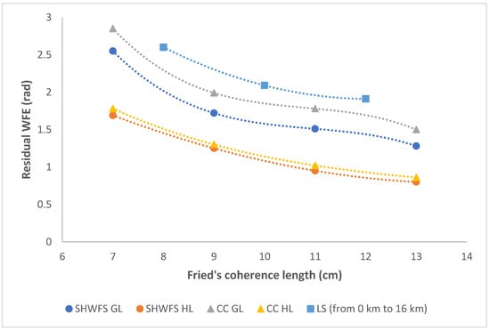
Figure 10.
Comparison of the residual WFE obtained by both ANN methods in comparison with the most used algorithm in real Solar AO system based on the least squares (LS) method. The data for the LS reconstruction are extracted from [33]. A polynomial trend line of order 3 has been added for each case. Note that the range of altitudes for the LS method is higher than for the other ones. The markers in the figure are fixed for each model for easier comprehension.
The difference remains when comparing higher values that are closer to real observation situations. Comparing the residual WFE obtained by these two new models with a 12 cm value with the LS one, the error obtained by the SHWFS ANN decreases by 21.8% for the ground layer comparison, while the FCN with CC as input also decreases by 11.7%. If the high-altitude layer is compared, the SHWFS FCN obtains 48.6% less error, and the CC FCN 47.1% less, according to Figure 10. Therefore, both FCN models achieve approximately only about half the error when operating in the worst turbulence situations. It is important to realize that the altitude layer cases for the FCNs were simulated between 9 and 12 km, while for the LS between 0 m and 16 km, being the mean of the altitudes, 8 km height was used.
Considering the comparisons in Figure 4 and Figure 5, the results shown in Figure 9 can be visually confirmed, as for each row, independently of the figure, the image on the left is more defined, similar to the center one, than the image on the right panel. Both images are of excellent quality reconstructions as both are parallel to the one in the center, having the high-phase difference zones in the same region of the image, and the same for the low-phase difference zones; however, the left one is always more detailed and precise than the right one.
Further, the recall time rounds to 4.5 ms per sample, very close to real-time computation. Note that the expected times for each correction of the whole system are usually considered under 2 ms [34], this approach being a solid candidate for real implementation. This can be supported by the fact that, although both the correlation-based approach and the SH image-based approach have similar recall times, the first one requires using time and resources to compute the correlations, adding a reason to determine the SH image-to-phase approach as the best choice. In general, those approaches save time that is usually required for other processes of AO, such as translating the SH images to correlations or centroids, and translating the outputs (usually Zernike coefficients or ideal centroids) to the phase [35]. The latest improvements are difficult to measure since they rely directly on the algorithm used.
5. Conclusions
In this research, AO reconstruction for solar scenarios was addressed. The proposed method relies on the numerical approximations performed by FCNs, which were trained successfully with simulated data, to predict turbulent profile phases. Two scenarios were considered: obtaining the phases from solar SH images, or from the images of the calculated correlations. The obtained results show how, considering performance, the network that uses images directly from the SH recovers phases that are numerically closer to the actual phase. Note that, in shape, both are quite similar. Moreover, the resolution that a DM can achieve for representing a phase is usually lower than the precision obtained by the methods presented here.
Anyway, both FCN methods obtain lower values of the residual WFE in comparison with the most common reconstruction algorithm currently used, the LS method. From the research, it can be extracted that the ANNs improved the residual WFE by 1% (lower) in the case of CC images and by 21% in the case of SH images.
However, the pre-processed images were shown to be more robust to variations than the solar SH images, allowing the CC FCN to be less susceptible to changes in the input data, since, after the cross-correlations are calculated, the resultant images have a similar pattern. As the CC FCN also obtained good-quality reconstructions, this renders cross-correlations a significant option as input data for ANN-based reconstructors when they are applied to non-trained situations, such as new turbulence conditions or observations in previously unknown solar regions.
In terms of similarity, both reconstructors based on FCNs showed very good performances in the reconstruction of high-altitude layers, achieving similarities higher than 93% in the worst case. This makes FCNs a very interesting option in more complex solar adaptive systems such as in multi-conjugated adaptive systems (MCAO), where several DMs are conjugated and each one only corrects determinate altitude layers; ANNs could take care of high-altitude layers due to their good performance for those cases.
Considering time requirements, both approaches are close to real-time computation, besides allowing for avoiding other algorithms that estimate intermediate values required for the reconstruction.
Possible future work related to this research involves the implementation of an optic bench for the subsequent implementation in a real solar telescope, such as the European Solar Telescope (EST). An optic bench will provide some realistic data to check the performance of the ANNs with real SH images or cross-correlations. However, with an optic bench, only a few several turbulence situations can be obtained, depending on the device available. Another future implementation is to develop the system for more complex AO configurations, such as ground layer adaptive optics (GLAO) or MCAO.
Author Contributions
F.G.R. and S.L.S.G. conceived and designed the study. C.G.-G. and F.G.R. contributed to the production of the simulations and the training of models. F.G.R. and E.D.A. performed the comparisons and analysis as well as the preparation of the manuscript. J.D.S. and S.L.S.G. contributed with interpretation of the results and with the preparation of the final version of the manuscript. All authors have read and agreed to the published version of the manuscript.
Funding
This research was funded by the Spanish Economy and Competitiveness Ministry with Grant Number AYA2017-89121-P.
Institutional Review Board Statement
Not applicable.
Informed Consent Statement
Not applicable.
Data Availability Statement
The data presented in this study are available on request from the corresponding author. The data are not publicly available due to their large size.
Conflicts of Interest
The authors declare no conflict of interest.
Abbreviations
| AI | Artificial Intelligence |
| ANN | Artificial Neural Network |
| AO | Adaptive Optics |
| CC | Cross-Correlations |
| CC GL | It refers to the ANN which reconstructs the ground layer that has as input the image of cross-correlations |
| CC HL | It refers to the ANN which reconstructs the high-altitude layer that has as input the image of cross-correlations |
| CCD | Charge-Coupled Device (camera used by the sensor) |
| CNN | Convolutional Neural Network |
| DASP | Durham Adaptive Optics Simulation Platform |
| DM | Deformable Mirror |
| FCN | Fully Convolutional Neural Network |
| GLAO | Ground Layer Adaptive Optics |
| LS | Least Squares |
| MCAO | Multi-Conjugated Adaptive Optics |
| MLP | Multilayer Perceptron |
| MOAO | Multi-Object Adaptive Optics |
| RMSE WFE | Root Mean Squared Error Wavefront Error |
| Fried’s Coherence Length | |
| SCAO | Single-Conjugated Adaptive Optics |
| SH, SHWFS | Shack–Hartmann Wavefront Sensor |
| SHWFS GL | It refers to the ANN which reconstructs the ground layer that has as input the information received by the Shack–Hartmann sensor |
| SHWFS HL | It refers to the ANN which reconstructs the high-altitude layer that has as input the information received by the Shack–Hartmann sensor |
| WFE | Wavefront Error |
| WFE net CC SHWFS | Wavefront error of the output of the network that has: The image of cross-correlations as input The image received by the Shack–Hartmann sensor as input |
| WFE residual CC SHWFS | Wavefront error of the difference between the simulated image and the output of the network that has: The image of cross-correlations as input The image received by the Shack–Hartmann sensor as input |
| WFE residual LS | Wavefront error of the difference between the simulated image and the reconstructed image by the least squares algorithm |
References
- Russell, S.J.; Norvig, P. Artificial Intelligence: A Modern Approach; Pearson Education Limited: Kuala Lumpur, Malaysia, 2016. [Google Scholar]
- Sands, T. Deterministic Artificial Intelligence; IntechOpen: London, UK, 2020. [Google Scholar]
- Sands, T. Development of Deterministic Artificial Intelligence for Unmanned Underwater Vehicles (UUV). J. Mar. Sci. Eng. 2020, 8, 578. [Google Scholar] [CrossRef]
- Smeresky, B.; Rizzo, A.; Sands, T. Optimal Learning and Self-Awareness Versus PDI. Algorithms 2020, 13, 23. [Google Scholar] [CrossRef] [Green Version]
- Batchelor, G.K. The Theory of Homogeneous Turbulence; Cambridge UP: London, UK, 1953. [Google Scholar]
- Zilberman, A.; Golbraikh, E.; Kopeika, N.S. Propagation of electromagnetic waves in Kolmogorov and non-Kolmogorov atmospheric turbulence: Three-layer altitude model. Appl. Opt. 2008, 47, 6385–6391. [Google Scholar] [CrossRef] [PubMed]
- Golbraikh, E.; Branover, H.; Kopeika, N.S.; Zilberman, A. Non-Kolmogorov atmospheric turbulence and optical signal propagation. Nonlinear Process. Geophys. 2006, 13, 297–301. [Google Scholar] [CrossRef]
- Osborn, J.; Guzman, D.; de Cos Juez, F.J.; Basden, A.G.; Morris, T.J.; Gendron, E.; Butterley, T.; Myers, R.M.; Guesalaga, A.; Sánchez Lasheras, F.; et al. Open-loop tomography with artificial neural networks on CANARY: On-sky results. Mon. Not. R. Astron. Soc. 2014, 441, 2508–2514. [Google Scholar] [CrossRef] [Green Version]
- Suárez Gómez, S.L.; González-Gutiérrez, C.; Díez Alonso, E.; Santos Rodríguez, J.D.; Sánchez Rodríguez, M.L.; Morris, T.; Osborn, J.; Basden, A.; Bonavera, L.; González-Nuevo González, J.; et al. Experience with Artificial Neural Networks applied in Multi-Object Adaptive Optics. Publ. Astron. Soc. Pac. 2019, 131, 108012. [Google Scholar] [CrossRef]
- Rimmele, T.R. Solar adaptive optics. In Proceedings of the Adaptive Optical Systems Technology, Munich, Germany, 7 July 2000; Volume 4007, pp. 218–232. [Google Scholar]
- García Riesgo, F.; Suárez Gómez, S.L.; Santos, J.D.; Diez Alonso, E.; Sánchez Lasheras, F. Overview and Choice of Artificial Intelligence Approaches for Night-Time Adaptive Optics Reconstruction. Mathematics 2021, 9, 1220. [Google Scholar] [CrossRef]
- Suárez-Gómez, S.L.; González-Gutiérrez, C.; Sánchez-Lasheras, F.; Basden, A.G.; Montilla, I.; De Cos Juez, F.J.; Collados-Vera, M. An approach using deep learning for tomographic reconstruction in solar observation. In Proceedings of the Adaptive Optics for Extremely Large Telescopes 5, Instituto de Astrofísica de Canarias (IAC), Tenerife, Spain, 25–30 June 2017. [Google Scholar]
- Sanchez Lasheras, F.; Ordóñez, C.; Roca-Pardiñas, J.; de Cos Juez, F.J. Real-time tomographic reconstructor based on convolutional neural networks for solar observation. Math. Methods Appl. Sci. 2020, 43, 8032–8041. [Google Scholar] [CrossRef]
- LeCun, Y.; Bengio, Y. Convolutional networks for images, speech, and time series. In The Handbook of Brain Theory and Neural Networks; A Bradford Book: Cambridge, MA, USA, 1995; pp. 255–258. [Google Scholar]
- Gardner, M.W.; Dorling, S.R. Artificial neural networks (the multilayer perceptron)—A review of applications in the atmospheric sciences. Atmos. Environ. 1998, 32, 2627–2636. [Google Scholar] [CrossRef]
- Giusti, A.; Ciresan, D.C.; Masci, J.; Gambardella, L.M.; Schmidhuber, J. Fast image scanning with deep max-pooling convolutional neural networks. In Proceedings of the Image Processing (ICIP), 2013 20th IEEE International Conference, Melbourne, Austrilia, 15–18 September 2013; pp. 4034–4038. [Google Scholar]
- Long, J.; Shelhamer, E.; Darrell, T. Fully convolutional networks for semantic segmentation. In Proceedings of the IEEE Conference on Computer Vision and Pattern Recognition, Boston, MA, USA, 7–12 June 2015; pp. 3431–3440. [Google Scholar]
- Chundi, G.S.; Lloyd-Hart, M.; Sundareshan, M.K. Training multilayer perceptron and radial basis function neural networks for wavefront sensing and restoration of turbulence-degraded imagery. In Proceedings of the 2004 IEEE International Joint Conference on Neural Networks, Budapest, Hungary, 25–29 July 2004; Volume 3, pp. 2117–2122. [Google Scholar]
- Keras Special Interest Group Keras Layer Activation Functions. Available online: https://keras.io/api/layers/activations/ (accessed on 11 March 2021).
- Nair, V.; Hinton, G.E. Rectified linear units improve restricted boltzmann machines. In Proceedings of the 27th International Conference on Machine Learning (ICML-10), Haifa, Israel, 21–24 June 2010; pp. 807–814. [Google Scholar]
- Zhang, Z.; Sabuncu, M. Generalized cross entropy loss for training deep neural networks with noisy labels. In Proceedings of the Advances in Neural Information Processing Systems, Montréal, QC, Canada, 3–8 December 2018; pp. 8778–8788. [Google Scholar]
- LeCun, Y.; Boser, B.; Denker, J.S.; Henderson, D.; Howard, R.E.; Hubbard, W.; Jackel, L.D. Backpropagation applied to handwritten zip code recognition. Neural Comput. 1989, 1, 541–551. [Google Scholar] [CrossRef]
- Chauvin, Y.; Rumelhart, D.E. Backpropagation: Theory, Architectures, and Applications; Psychology Press: Hove, UK, 2013. [Google Scholar]
- Ruder, S. An overview of gradient descent optimization algorithms. arXiv Prepr. 2016, arXiv:1609.04747. [Google Scholar]
- Nesterov, Y. Lectures on Convex Optimization; Springer: Berlin/Heidelberg, Germany, 2018; Volume 137. [Google Scholar]
- Suárez Gómez, S.L.; García Riesgo, F.; González Gutiérrez, C.; Rodríguez Ramos, L.F.; Santos, J.D. Defocused Image Deep Learning Designed for Wavefront Reconstruction in Tomographic Pupil Image Sensors. Mathematics 2021, 9, 15. [Google Scholar] [CrossRef]
- Davies, R.; Kasper, M. Adaptive optics for astronomy. Annu. Rev. Astron. Astrophys. 2012, 50, 305–351. [Google Scholar] [CrossRef] [Green Version]
- Osborn, J.; Guzman, D.; de Cos Juez, F.J.; Basden, A.G.; Morris, T.J.; Gendron, É.; Butterley, T.; Myers, R.M.; Guesalaga, A.; Sanchez Lasheras, F.; et al. First on-sky results of a neural network based tomographic reconstructor: Carmen on Canary. In Proceedings of the SPIE Astronomical Telescopes and Instrumentation, Montréal, QC, Canada, 25–26 June 2014; Marchetti, E., Close, L.M., Véran, J.-P., Eds.; International Society for Optics and Photonics: Bellingham, WA, USA, 2014; p. 91484M. [Google Scholar]
- Von Der Lühe, O.; Widener, A.L.; Rimmele, T.; Spence, G.; Dunn, R.B. Solar feature correlation tracker for ground-based telescopes. Astron. Astrophys. 1989, 224, 351–360. [Google Scholar]
- Bracewell, R.N.; Bracewell, R.N. The Fourier Transform and Its Applications; McGraw-Hill: New York, NY, USA, 1986; Volume 31999. [Google Scholar]
- Basden, A.G.; Bharmal, N.A.; Jenkins, D.; Morris, T.J.; Osborn, J.; Peng, J.; Staykov, L. The Durham Adaptive Optics Simulation Platform (DASP): Current status. SoftwareX 2018, 7, 63–69. [Google Scholar] [CrossRef]
- Berkefeld, T.; Schmidt, D.; Soltau, D.; von der Lühe, O.; Heidecke, F. The GREGOR adaptive optics system. Astron. Nachrichten 2012, 333, 863–871. [Google Scholar] [CrossRef]
- Riesgo, F.G.; Gómez, S.L.S.; Rodríguez, J.D.S.; Gutiérrez, C.G.; Alonso, E.D.; Rodríguez, F.J.I.; Fernández, P.R.; Bonavera, L.; Menéndez, S.d.C.; de Cos Juez, F.J. Early Fully-Convolutional Approach to Wavefront Imaging on Solar Adaptive Optics Simulations. In Proceedings of the International Conference on Hybrid Artificial Intelligence Systems, Gijón, Spain, 11–13 November 2020; pp. 674–685. [Google Scholar]
- González-Gutiérrez, C.; Sánchez-Rodríguez, M.L.; Calvo-Rolle, J.L.; de Cos Juez, F.J. Multi-GPU Development of a Neural Networks Based Reconstructor for Adaptive Optics. Complexity 2018, 2018, 5348265. [Google Scholar] [CrossRef]
- Guzmán, D.; de Cos Juez, F.J.; Myers, R.; Guesalaga, A.; Lasheras, F.S. Modeling a MEMS deformable mirror using non-parametric estimation techniques. Opt. Express 2010, 18, 21356–21369. [Google Scholar] [CrossRef] [PubMed]
Publisher’s Note: MDPI stays neutral with regard to jurisdictional claims in published maps and institutional affiliations. |
© 2021 by the authors. Licensee MDPI, Basel, Switzerland. This article is an open access article distributed under the terms and conditions of the Creative Commons Attribution (CC BY) license (https://creativecommons.org/licenses/by/4.0/).