On the Amplitude Amplification of Quantum States Corresponding to the Solutions of the Partition Problem

Abstract

In this paper we investigate the effects of a quantum algorithm which increases the amplitude of the states corresponding to the solutions of the partition problem by a factor of almost two. The study is limited to one iteration.

1. Introduction and Preliminaries

Quantum computing promises to offer a different paradigm for solving long standing complex problems. Shor’s algorithm [1] is a clear example of the success of the application of quantum computation to a difficult problem, the factoring of integers. Other algorithms like Deutsch-Josza’s [2] or Grover’s [3] give strong hints that the intrinsic parallelism of quantum computation could be used in order to efficiently solve computationally complex problems. In particular, Grover’s algorithm uses the concept of an oracle $f(x)$ which, given a configuration x of the problem at hand, computes whether or not x is a solution of the problem. In other words, if x is a configuration that solves an instance of a combinatorial problem then the oracle returns $f(x)=1$ otherwise the oracle outputs $f(x)=0$. By using this oracle, Grover’s algorithm is capable of speeding up the time to search for a solution of many, very complex, combinatorial problems. In Grover’s algorithm the Grover iteration amplifies the amplitude of the configuration states corresponding to solutions of the problem (i.e., those states x for which $f(x)=1$) by a factor less than $O(1/\sqrt{N})$ (in the worst case in which there is only one configuration which is the solution of the problem), where $N=2^n$ is the number of possible configurations. In this way, after approximately $O(\sqrt{N})$ iterations, the amplitudes of the states corresponding to the solutions of the problem approach 1.

We exploit the parallelism of quantum computation, therefore devising a quantum algorithm that is capable of doubling the amplitude of the states corresponding to the solution of a problem. In this paper, we will focus on the subset sum problem, a well known NP-complete problem. The subset sum problem is very important both at a theoretical level in complexity theory, and at a practical level in applications such as cryptography. The problem can be stated in the following way in which we denote by ${\mathbb{N}}^{+}$, the set of non-zero natural numbers. Let E be a finite set of elements, $s:E\to {\mathbb{N}}^{+}$ a function and $W\in {\mathbb{N}}^{+}$ a target number. The subset sum problem wonders whether there exists a subset $E^{\prime }\subset E$ such that ${\sum }_{e\in E^{\prime }}s(e)=W$. Usually this problem can also be reformulated as follows. There exists a subset $E^{\prime }\subset E$ such that ${\sum }_{e\in E^{\prime }}s(e)={\sum }_{e\in E\setminus E^{\prime }}s(e)$? In this later formulation it is called the partition problem (PP) [4]. From now on we do not lose any generality in considering the set E equals the set of the first $\left|E\right|$ natural numbers; that is, we always consider $E=\{0,1,\dots ,n-1\}$. Furthermore, we note that if PP has a solution $E^{\prime }$ then $E-E^{\prime }$ is also a solution of the PP.

The literature is abundant in the study of this problem, for which the dynamic programming solving strategy is the most commonly applied. More recently, it has also been approached from the point of view of quantum computing, among these references we can mention [5] where an instance of the subset sum problem can be implemented by a quantum algorithm using the nuclear magnetic resonance (NMR) technique. In that paper, even at a very early stage and with a low number of qubits, they limit themselves to showing that the problem can be approached from this new perspective.

In [6], the authors studied the problem through both an asymptotic heuristic and a new data structure for using quantum gates. There, the possibility of obtaining an improvement over classical algorithms is shown, specifically the Howgrave–Graham–Joux [7], which of course is fully coherent with the NP ⊆ BQP conjecture, obtaining a bound time $\tilde{O}(2^{2/3n})$.

More recently, in 2018, Helm and May [8] proposed a quantum algorithm that reduces the heuristic time to $\tilde{O}(2^{0.226n})$. A couple of years later, Li and Li [9] reduced this time beyond that, i.e., to $\tilde{O}(2^{0.209n})$.

In this work we will get rid of the heuristics of these studies to better go for the modest approach of [5]. In this sense, we propose a piece of quantum code using a quantum circuit to model the problem, consequently we devise a transformation that will allow us to increase the amplitudes of those corresponding to the solution by $50\%$, leaving the line of how and how many times this process could be iterated, as the key issue to be dealt with. In fact, we think that we could find the same limitations as those from Grover’s algorithm. Anyway, we believe that this line of research deserves to be addressed.

Let $x\in \mathbb{N}$, $0\le x<2^n$ then we say that $|x\rangle$ is a computational state, the binary representation of which is $|x_{n-1}{x}_{n-2}\dots x_0\rangle$ with $x_{n-1}$ being the most significant bit of the binary representation of $|x\rangle$.

The S gate for a single qubit is represented by the following matrix:

$$S=\left[\begin{array}{cc}1& 0\\ 0& i\end{array}\right]$$

Other usual gates are Pauli X gate, also known as NOT gates, and $\sqrt{X}$ gates.

$$X=\left[\begin{array}{cc}0& 1\\ 1& 0\end{array}\right]\sqrt{X}=\frac{1}{2}\left[\begin{array}{cc}1+i& 1-i\\ 1-i& 1+i\end{array}\right]$$

The Hadamard gate for a single qubit is

$$H=\frac{\sqrt{2}}{2}\left[\begin{array}{cc}1& 1\\ 1& -1\end{array}\right]$$

While the same gate for n qubits is represented by the following matrix

$$H^{{\otimes }^n}=\underset{i=1}{\overset{n}{⨂}}\frac{\sqrt{2}}{2}\left[\begin{array}{cc}1& 1\\ 1& -1\end{array}\right]$$

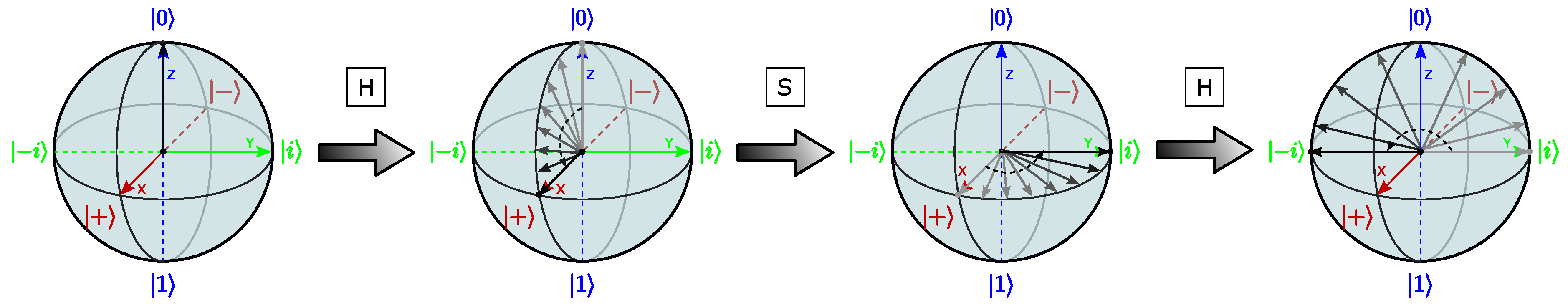
As stated before, we are interested in amplifying amplitudes for the search problem. In order to do this we make use of sequences of quantum gates in the way of Hadamard-S-Hadamard. Let us start by describing graphically the effect of such quantum gates and so resorting to the positions of the state vector represented in the Bloch sphere.

The effect of applying an H q-gate over a qubit represented on the Bloch Sphere can be seen as “first rotating an angle of $\pi$ radians around the Z axis and then rotating an angle of $\frac{\pi }{2}$ radians around the Y axis” (fully equivalent to “first rotating an angle of $\frac{\pi }{2}$ radians around the Y axis and then rotating an angle of $\pi$ radians around the X axis”, which are the movements made by H in Figure 1). Hadamard q-gate application changes a qubit from a computational basis to a Hadamard basis. To better understand the effects of the sequence H-S-H we start, as usual, from a qubit initialized to $|0\rangle$, i.e., located at the north pole of the Bloch s. which, moved through a Hadamard gate, gets located at the equator of the Bloch s., specifically on the X axis, in the position usually known as a $|+\rangle$, which corresponds to the qubit

$$|+\rangle =\frac{\sqrt{2}}{2}|0\rangle +\frac{\sqrt{2}}{2}|1\rangle$$

After this gate, we apply an S gate, the effect of which is a rotation of the state vector through an angle of $\frac{\pi }{2}$ radians around the Z axis. This places the qubit at position $|i\rangle$.

$$|i\rangle =\frac{\sqrt{2}}{2}|0\rangle +i·\frac{\sqrt{2}}{2}|1\rangle$$

Finally, the effect of the second application of gate H is to reset the computational base, and then the vector from position $|i\rangle$ moves to the opposite point on the Y axis, that is, to the position

$$|-i\rangle =\frac{\sqrt{2}}{2}|0\rangle -i·\frac{\sqrt{2}}{2}|1\rangle$$

In general, we have the following result

$$\begin{array}{ccc}HSH\hfill & =\hfill & \sqrt{X}\hfill \end{array}$$

That is, an HSH gate is equivalent to a $\frac{\pi }{2}$ radians clockwise rotation around the X axis as Figure 1 shows over a single qubit initialized to $|0\rangle$.

Let us go for the general case of a qubit register initialized, as usual, to ${|0\rangle }^{{\otimes }^n}$.

2. The Effect of Applying Hadamard-S-Hadamard Gates to ${|\mathbf{0}\rangle }^{{\otimes }^{\mathit{n}}}$

First of all we will introduce a notation which will be heavily used in the rest of the paper. Let $x\in \mathbb{N}$, $0\le x<2^n$ and $x_{n-1}\dots ,x_1{x}_0$ be its binary representation. The Hamming weight of x will be denoted as $w(x)={\sum }_{j=0}^{n-1}{x}_j$. Let $z\in \mathbb{N}$, $0\le z<2^n$, $|z\rangle =|z_{n-1}{z}_{n-2}\dots z_0\rangle$. The term $x·z$ denotes ${\sum }_{j=0}^{n-1}{x}_j{z}_j$. Furthermore, $\forall k\in \mathbb{N}$, $0<k<n$, we denote by $z_{\text{-}\mathrm{k}}$ a natural number obtained from z by considering only the least $n-k$ significant bits, that is, the binary representation of $z_{\text{-}\mathrm{k}}$ is $z_{n-k-1}{z}_{n-k-2}\dots z_0$. In other words $z_{\text{-}\mathrm{k}}$ is the bitwise AND between z and $2^{n-k}-1$.

In this section we want to determine the effect of applying Hadamard first, then S and finally Hadamard gates on quantum state ${|0\rangle }^{{\otimes }^n}$, that is, we want to determine a formula for $|\alpha \rangle$ such that

$$|\alpha \rangle =H^{{\otimes }^n}{S}^{{\otimes }^n}{H}^{{\otimes }^n}{|0\rangle }^{{\otimes }^n}$$

(1)

and we show that in the out-coming computational state $|\alpha \rangle ={\sum }_{z=0}^{2^n-1}{a}_z|z\rangle$ the amplitude $a_z$ of a single state $|z\rangle$ depends just on $w(z)$.

It is well known, see [3], that given any computational state $|x\rangle$ where $0\le x<2^n$

$$|\psi \rangle =H^{{\otimes }^n}|x\rangle ={\displaystyle \frac{1}{\sqrt{2^n}}}\sum _{z=0}^{2^n-1}{(-1)}^{x·z}|z\rangle$$

(2)

Now we start with the following Lemma

Lemma 1.

Let $0\le x<2^n$

$$S^{{\otimes }^n}|x\rangle =i^{w(x)}|x_{n-1}{x}_{n-2}\dots x_0\rangle$$

Proof. 

Induction on n is the base case with $n=1$ straightforward. So suppose that the statement holds for $n-1$. Then

$$\begin{array}{cc}\hfill S^{{\otimes }^n}|x\rangle & =S|x_{n-1}\rangle \otimes S|x_{n-2}\rangle \dots \otimes S|x_0\rangle =S^{{\otimes }^{n-1}}|x_{n-1}\dots x_1\rangle \otimes S|x_0\rangle =\hfill \\ \hfill & =i^{{\sum }_{j=1}^{n-1}{x}_j}|x_{n-1}\dots x_1\rangle \otimes S|x_0\rangle =(\mathrm{by}\mathrm{induction}\mathrm{hypothesis})\hfill \\ \hfill & =i^{{\sum }_{j=1}^{n-1}{x}_j}|x_{n-1}\dots x_1\rangle \otimes i^{x_0}|x_0\rangle =\hfill \\ \hfill & =i^{w(x)}|x_{n-1}{x}_{n-2}\dots x_0\rangle \hfill \end{array}$$

□

Now by Lemma 1 and Equation (2), we have that

$$\begin{array}{c}\hfill |{\psi }_1\rangle =S^{{\otimes }^n}{H}^{{\otimes }^n}{|0\rangle }^{{\otimes }^n}=S^{{\otimes }^n}{\displaystyle \frac{1}{\sqrt{2^n}}}\sum _{x=0}^{2^n-1}|x\rangle ={\displaystyle \frac{1}{\sqrt{2^n}}}\sum _{x=0}^{2^n-1}{i}^{w(x)}|x\rangle \end{array}$$

and applying the Hadamard to $|{\psi }_1\rangle$, by (2), we have that

$$\begin{array}{c}\hfill |{\psi }_2\rangle =H^{{\otimes }^n}|{\psi }_1\rangle ={\displaystyle \frac{1}{\sqrt{2^n}}}\sum _{x=0}^{2^n-1}{i}^{w(x)}\left[{\displaystyle \frac{1}{\sqrt{2^n}}}\sum _{z=0}^{2^n-1}{(-1)}^{x·z}|z\rangle \right]\end{array}$$

and reordering the term of the sum we have that

$$\begin{array}{c}\hfill |{\psi }_2\rangle ={\displaystyle \frac{1}{2^n}}\sum _{z=0}^{2^n-1}\sum _{x=0}^{2^n-1}{(-1)}^{x·z}{i}^{w(x)}|z\rangle ={\displaystyle \frac{1}{2^n}}\sum _{z=0}^{2^n-1}\left(\sum _{x=0}^{2^n-1}{i}^{w(x)}{(-1)}^{x·z}\right)|z\rangle \end{array}$$

So in order to compute the amplitudes of $|{\psi }_2\rangle$ we need to compute the sum

$$\sum _{x=0}^{2^n-1}{i}^{w(x)}{(-1)}^{x·z}$$

(3)

for every $0\le z<2^n$. We will do this in the following two theorems. First of all we need the next Lemma which will be heavily used in the rest of the paper.

Lemma 2.

Let $0\le z<2^{2m+1}$ and $0\le x<2^{2m+1}$ and let $z_{2m}{z}_{2m-1}\dots z_0$ and $x_{2m}{x}_{2m-1}\dots x_0$ be the binary representation, respectively, of z and x. We have that

$$\begin{array}{cc}\hfill \sum _{x=2^{2m}}^{2^{2m+1}-1}& i^{w(x)}{(-1)}^{{\sum }_{j=0}^{2m}{z}_j·x_j}=i{(-1)}^{z_{2m}}\sum _{x=0}^{2^{2m}-1}{i}^{w(x)}{(-1)}^{{\sum }_{j=0}^{2m-1}{z}_j·x_j}\hfill \end{array}$$

(4)

Proof. 

We note that, on the left hand of Equation (4), for every element of the sum, we have that $x_{2m}=1$. Therefore ${\sum }_{j=0}^{2m}{z}_j·x_j={\sum }_{j=0}^{2m-1}{z}_j·x_j+z_{2m}$. Based on this we have that

$$\begin{array}{cc}\hfill \sum _{x=2^{2m}}^{2^{2m+1}-1}& i^{w(x)}{(-1)}^{{\sum }_{j=0}^{2m}{z}_j·x_j}={(-1)}^{z_{2m}}\sum _{x=2^{2m}}^{2^{2m+1}-1}{i}^{w(x)}{(-1)}^{{\sum }_{j=0}^{2m-1}{z}_j·x_j}\hfill \end{array}$$

Furthermore for the same reason above, if $2^{2m}\le x<2^{2m+1}$ and if $0\le \overline{x}<2^{2m}$ then we have that $w(x)=w(\overline{x})+1$ and this proves Equation (4). □

Theorem 1.

Let $0\le z<2^n$, $z\in \mathbb{N}$. If $n=2m$ is even we have that

$$\sum _{x=0}^{2^n-1}{i}^{w(x)}{(-1)}^{z·x}={(-1)}^{w(z)}{i}^{m+w(z)}{2}^m$$

(5)

Proof. 

We prove Equation (5) on induction on m being the base case with $m=1$ being easily verifiable for all $z\in \{0,1,2,3\}$. So suppose the statement holds for all $h\le m$ and for all $0\le z<2^{2m}$. Then, for any $0\le z<2^{2m+2}$ we have

$$\begin{array}{cc}\hfill \sum _{x=0}^{2^{2m+2}-1}{i}^{w(x)}{(-1)}^{z·x}=& \sum _{x=0}^{2^{2m}-1}{i}^{w(x)}{(-1)}^{{\sum }_{j=0}^{2m-1}{z}_j·x_j}\hfill \end{array}$$

(6)

$$\begin{array}{cc}\hfill +& \sum _{x=2^{2m}}^{2^{2m+1}-1}{i}^{w(x)}{(-1)}^{{\sum }_{j=0}^{2m}{z}_j·x_j}+\hfill \end{array}$$

(7)

$$\begin{array}{cc}\hfill +& \sum _{x=2^{2m+1}}^{2^{2m+2}-1}{i}^{w(x)}{(-1)}^{{\sum }_{j=0}^{2m+1}{z}_j·x_j}\hfill \end{array}$$

(8)

Now, by Equation (4) and by induction hypothesis, we have that (7) is equal to

$$\begin{array}{cc}\hfill \sum _{x=2^{2m}}^{2^{2m+1}-1}& i^{w(x)}{(-1)}^{{\sum }_{j=0}^{2m}{z}_j·x_j}=i{(-1)}^{z_{2m}}\sum _{x=0}^{2^{2m}-1}{i}^{w(x)}{(-1)}^{{\sum }_{j=0}^{2m-1}{z}_j·x_j}=\hfill \\ \hfill & =i{(-1)}^{z_{2m}}{(-1)}^{w(z_{\text{-}2})}{i}^{m+w(z_{\text{-}2})}{2}^m\hfill \end{array}$$

(9)

Likewise, in the term (8), for each, x is the sum, the bit $x_{2m+1}$ is always set to 1, so we have that (8) is, by Equation (4), equal to

$$\begin{array}{cc}\hfill \sum _{x=2^{2m+1}}^{2^{2m+2}-1}& i^{w(x)}{(-1)}^{{\sum }_{j=0}^{2m+1}{z}_j·x_j}=i{(-1)}^{z_{2m+1}}\sum _{x=0}^{2^{2m+1}-1}{i}^{w(x)}{(-1)}^{{\sum }_{j=0}^{2m}{z}_j·x_j}\hfill \end{array}$$

(10)

Now by repeatedly applying Equation (4) and the induction hypothesis we have that the sum in the right hand of Equation (10) is

$$\begin{array}{cc}\hfill \sum _{x=0}^{2^{2m+1}-1}& i^{w(x)}{(-1)}^{{\sum }_{j=0}^{2m}{z}_j·x_j}=\hfill \\ \hfill =& \sum _{x=0}^{2^{2m}-1}{i}^{w(x)}{(-1)}^{{\sum }_{j=0}^{2m-1}{z}_j·x_j}+\sum _{x=2^{2m}}^{2^{2m+1}-1}{i}^{w(x)}{(-1)}^{{\sum }_{j=0}^{2m}{z}_j·x_j}=\hfill \end{array}$$

(11)

$$\begin{array}{cc}\hfill & ={(-1)}^{w(z_{\text{-}2})}{i}^{m+w(z_{\text{-}2})}{2}^m+i{(-1)}^{z_{2m}}\sum _{x=0}^{2^{2m}-1}{i}^{w(x)}{(-1)}^{{\sum }_{j=0}^{2m-1}{z}_j·x_j}=\hfill \\ \hfill & ={(-1)}^{w(z_{\text{-}2})}{i}^{m+w(z_{\text{-}2})}{2}^m\left[1+i{(-1)}^{z_{2m}}\right]\hfill \end{array}$$

(12)

So if we replace (12) in (10) and if we sum together (6), (9) and (10) we obtain

$$\begin{array}{cc}\hfill a_z=& {(-1)}^{w(z_{\text{-}2})}{i}^{m+w(z_{\text{-}2})}{2}^m\left[1+i{(-1)}^{z_{2m}}+i{(-1)}^{z_{2m+1}}+i^2{(-1)}^{z_{2m}+z_{2m+1}}\right]=\hfill \\ \hfill =& {(-1)}^{w(z_{\text{-}2})}{i}^{m+1+w(z_{\text{-}2})}{2}^m\left[-i+{(-1)}^{z_{2m}}+{(-1)}^{z_{2m+1}}+i{(-1)}^{z_{2m}+z_{2m+1}}\right]\hfill \end{array}$$

(13)

Now if we denote by $P={(-1)}^{w(z_{\text{-}2})}{i}^{m+1+w(z_{\text{-}2})}{2}^m$ we have that (13) is

$$\begin{array}{c}\hfill a_z=\left\{\begin{array}{cc}\hfill 2P& \mathrm{if}{z}_{2m}=z_{2m+1}=0\hfill \\ \hfill -2iP& \mathrm{if}{z}_{2m}\ne z_{2m+1}\hfill \\ \hfill -2P& \mathrm{if}{z}_{2m}=z_{2m+1}=1\hfill \end{array}\right.\end{array}$$

and it is now easy to verify that

$$a_z={(-1)}^{w(z)}{i}^{m+1+w(z)}{2}^{m+1}$$

for every $0\le z<2^{2m+2}$, and this proves the induction step. □

Theorem 2.

Let $n=2m+1$ be an odd natural, $m\in \mathbb{N}$ and let $0\le z<2^n$, $z\in \mathbb{N}$. Then

$$\sum _{x=0}^{2^n-1}{i}^{w(x)}{(-1)}^{z·x}={(-1)}^{w(z)}{i}^{m+w(z)}{2}^m(1+i)$$

(14)

Proof. 

First of all we note that Equation (14) holds if $m=0$ and $z\in \{0,1\}$. So in the following we suppose that $m>1$. We have that

$$\begin{array}{cc}\hfill a_z& =\sum _{x=0}^{2^{2m+1}-1}{i}^{w(x)}{(-1)}^{z·x}=\hfill \\ \hfill =& \sum _{x=0}^{2^{2m}-1}{i}^{w(x)}{(-1)}^{{\sum }_{j=0}^{2m-1}{z}_j·x_j}+\sum _{x=2^{2m}}^{2^{2m+1}-1}{i}^{w(x)}{(-1)}^{{\sum }_{j=0}^{2m}{z}_j·x_j}\hfill \end{array}$$

and, by Theorem 1, and by Equation (4), we have

$$\begin{array}{cc}\hfill a_z& ={(-1)}^{w(z_{\text{-}1})}{i}^{m+w(z_{\text{-}1})}{2}^m+i{(-1)}^{z_{2m}}\sum _{x=0}^{2^{2m}-1}{i}^{w(x)}{(-1)}^{{\sum }_{j=0}^{2m-1}{z}_j·x_j}=\hfill \\ \hfill =& {(-1)}^{w(z_{\text{-}1})}{i}^{m+w(z_{\text{-}1})}{2}^m+i{(-1)}^{z_{2m}}{(-1)}^{w(z_{\text{-}1})}{i}^{m+w(z_{\text{-}1})}{2}^m=\hfill \\ \hfill =& {(-1)}^{w(z_{\text{-}1})}{i}^{m+w(z_{\text{-}1})}{2}^m\left[1+i{(-1)}^{z_{2m}}\right]\hfill \end{array}$$

(15)

Let $z_{2m}{z}_{2m-1}\dots z_0$ be the binary representation of z. Suppose first that $z_{2m}=0$. Then Equation (15) become

$${(-1)}^{w(z)}{i}^{m+w(z)}{2}^m+{(-1)}^{w(z)}{i}^{m+w(z)+1}{2}^m$$

(16)

and the Theorem is therefore proved. So suppose that $z_{2m}=1$. Then Equation (15) become

$${(-1)}^{w(z)-1}{i}^{m+w(z)-1}{2}^m+{(-1)}^{w(z)}{i}^{m+w(z)}{2}^m$$

(17)

but observing that

$${(-1)}^{w(z)}{i}^{m+w(z)+1}={(-1)}^{w(z)-1}{i}^{m+w(z)-1}$$

(18)

we have that also in this case the theorem is satisfied. □

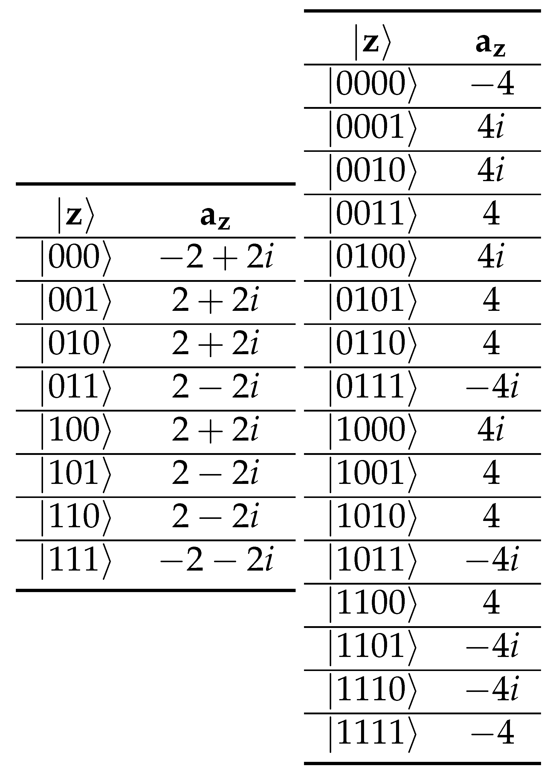
As an example we have computed the amplitudes $a_z$ (disregarding the normalization factor) for $n\in \{3,4\}$ and we report them on Figure 2.

3. Doubling the Amplitudes of the Solution States of the PP

In this section we consider a quantum circuit for doubling the amplitude of the solution’s states of the partition problem.

We describe an application of the gates described in the previous section in a quantum circuit to deal with PP (see Figure 3). While the following results apply specifically to the PP, they can be applied to any other search problem.

Let us denote ${\sum }_{e\in E}s(e)/2$ by $\mathcal{S}$. Notice that S belonging to $\mathbb{Z}$ is a requirement for PP to have a solution. We use the two’s complement representation of $-\mathcal{S}$, so requiring for it $m=\lceil {log}_2\mathcal{S}\rceil +1$ qubits. Then for each $e\in E$, we use $k_e=\lfloor {log}_{2}s(e)\rfloor +1$ qubits to encode $s(e)$. These qubits will remain constant in every phase of the circuit and therefore we will not consider them in the rest of the discussion. As usual, we use n qubits to encode a subset $E^{\prime }$ of E, i.e., if $|x_{n-1}{x}_{n-2}\dots x_0\rangle$ is the state of those n qubits, then an element e, $0\le e<n$, is included in the set $E^{\prime }$ if and only if $x_e=1$. We will use m qubits, denoted in the following by $|\sigma \rangle$, to store the sum $\sigma =-\mathcal{S}+{\sum }_{e\in E^{\prime }}s(e)$ for the elements selected in $|x\rangle$. In this way $|\sigma \rangle ={|0\rangle }^{{\otimes }^m}$ for a solution $|x\rangle$ of the PP. Qubit $|c\rangle$ is used for control purposes.

For a top-down description we can distinguish four groups of bits: $|x\rangle$, $|\sigma \rangle$, $|c\rangle$ and the sets of qubits used to represent the constants $s(e)$ for each element of E. Note that the number of qubits of the circuit, $n+m+1+{\sum }_{e\in E}{k}_e$, is polynomial in the size of a concise specification of the PP.

At the beginning of the circuit we have the superposition:

$$\begin{array}{c}\hfill |{\phi }_0{\rangle =|0\rangle }^{{\otimes }^n}|\sigma \rangle |c\rangle \end{array}$$

where $\sigma$ is set to the two’s complement of $-\mathcal{S}$ and $|c\rangle$ is set to $|1\rangle$. Then, we apply the Hadamard q-gate to the first n qubits, so obtaining

$$\begin{array}{cc}\hfill |{\phi }_1\rangle & =\left(H^{{\otimes }^n}\otimes I^{m+1}\right)|{\phi }_0\rangle ={\displaystyle \frac{1}{\sqrt{2^n}}}\sum _{x=0}^{2^n-1}|x\rangle |\sigma \rangle |c\rangle \hfill \end{array}$$

Next, we use each qubit $x_e$ to conditionally sum the element $s(e)$ to $|\sigma \rangle$. If there exists a solution to the PP then, in the final superposition of $|\sigma \rangle$, the amplitude of the state ${|x\rangle |0\rangle }^{{\otimes }^m}|c\rangle$ will not be 0. The states $|x\rangle$ for which $|\sigma \rangle$ is zero will be referred to as the solutions states of the PP. The control qubit $|c\rangle$ will be set to zero exactly for those states for which $|\sigma \rangle ={|0\rangle }^{{\otimes }^m}$. At this point we apply an uncomputational step in order to set $|\sigma \rangle =|-\mathcal{S}\rangle$. Now if we apply the S gate to the first n qubits we obtain, by Lemma 1

$$\begin{array}{cc}\hfill |{\phi }_2\rangle & =\left(S^{{\otimes }^n}\otimes I^{m+1}\right)|{\phi }_1\rangle ={\displaystyle \frac{1}{\sqrt{2^n}}}\sum _{x=0}^{2^n-1}{i}^{w(x)}|x\rangle |\sigma \rangle |c\rangle \hfill \end{array}$$

Afterwards Hadamard gate is applied to the first n qubits controlled by the control qubit $|c\rangle$ such that it only affects non-solution states (see Figure 3). For the sake of simplicity we suppose that PP has only two solutions whose numeric representation is y and its bitwise complement $\overline{y}$. By Equation (3), we obtain

$$\begin{array}{cc}\hfill |{\phi }_2\rangle & \stackrel{\mathrm{contr}{H}^{{\otimes }^n}}{\to }|{\phi }_3\rangle ={\displaystyle \frac{1}{\sqrt{2^n}}}\sum _{z\in \{y,\overline{y}\}}{i}^{w(z)}|z\rangle |\sigma \rangle |0\rangle +\hfill \\ \hfill +& {\displaystyle \frac{1}{2^n}}\sum _{z=0}^{2^n-1}\sum _{x\notin \{y,\overline{y}\}}{i}^{w(x)}{(-1)}^{x·z}|z\rangle |\sigma \rangle |1\rangle =\hfill \\ \hfill =& {\displaystyle \frac{1}{2^n}}\left[\sqrt{2^n}\sum _{z\in \{y,\overline{y}\}}{i}^{w(z)}|z\rangle |\sigma \rangle |0\rangle +\sum _{z=0}^{2^n-1}\sum _{x\notin \{y,\overline{y}\}}{i}^{w(x)}{(-1)}^{x·z}|z\rangle |\sigma \rangle |1\rangle \right]\hfill \end{array}$$

(19)

Now we want to quantify the amplitude of the state $|y\rangle |\sigma \rangle |1\rangle$ and $|\overline{y}\rangle |\sigma \rangle |1\rangle$ of Equation (19). We consider only the state $|y\rangle |\sigma \rangle |1\rangle$ since the same arguments can be applied to state $|\overline{y}\rangle |\sigma \rangle |1\rangle$. The amplitude $b_y$ of the state $|y\rangle |\sigma \rangle |1\rangle$ (in the following we disregard the normalization factor $1/2^n$) is given by the following formula

$$\begin{array}{c}\hfill b_y=\sum _{x\notin \{y,\overline{y}\}}{i}^{w(x)}{(-1)}^{x·y}\end{array}$$

(20)

We may write the above sum as

$$\begin{array}{c}\hfill b_y=\sum _{x\notin \{y,\overline{y}\}}{i}^{w(x)}{(-1)}^{x·y}=\sum _{x=0}^{2^n-1}{i}^{w(x)}{(-1)}^{x·y}-\sum _{x\in \{y,\overline{y}\}}{i}^{w(x)}{(-1)}^{x·y}\end{array}$$

(21)

We have that

$$\begin{array}{cc}\hfill \sum _{x\in \{y,\overline{y}\}}{i}^{w(x)}{(-1)}^{x·y}& =i^{w(y)}{(-1)}^{y·y}+i^{n-w(y)}{(-1)}^{\overline{y}·y}=\hfill \\ \hfill =& i^{w(y)}{(-1)}^{w(y)}+i^{n-w(y)}=\hfill \end{array}$$

(22)

Then, recalling that $i^x=i^{-x}$ when x is even and $i^{-x}=-i^x$ when x is odd, we have two cases:

• $w(y)$ is even

  $$\begin{array}{cc}\hfill i^{w(y)}{(-1)}^{w(y)}& +i^{n-w(y)}=i^{w(y)}{(-1)}^{w(y)}+i^{n+w(y)}=\hfill \\ \hfill & =i^{w(y)}(1+i^n)\hfill \end{array}$$

  (23)
• $w(y)$ is odd

  $$\begin{array}{cc}\hfill i^{w(y)}{(-1)}^{w(y)}& +i^{n-w(y)}=i^{w(y)}{(-1)}^{w(y)}-i^{n+w(y)}=\hfill \\ \hfill & =-i^{w(y)}(1+i^n)\hfill \end{array}$$

  (24)

For simplicity of notation in the following we denote $w(y)$ as simply $\overline{w}$. We have that if $n=2m$ is even then, by Theorem 1, $b_y$ is

$$\begin{array}{c}\hfill b_y=\left\{\begin{array}{cc}{(-1)}^{\overline{w}}{i}^{m+\overline{w}}{2}^m-i^{\overline{w}}(1+i^{2m})\hfill & \mathrm{if}\overline{w}\mathrm{is}\mathrm{even}\hfill \\ \hfill & \\ {(-1)}^{\overline{w}}{i}^{m+\overline{w}}{2}^m+i^{\overline{w}}(1+i^{2m})\hfill & \mathrm{if}\overline{w}\mathrm{is}\mathrm{odd}\hfill \end{array}\right.\end{array}$$

(25)

while if $n=2m+1$ is odd, by Theorem 2, $b_y$ is

$$\begin{array}{c}\hfill b_y=\left\{\begin{array}{cc}{(-1)}^{\overline{w}}{i}^{m+\overline{w}}{2}^m(1+i)-i^{\overline{w}}(1+i^{2m+1})\hfill & \mathrm{if}\overline{w}\mathrm{is}\mathrm{even}\hfill \\ \hfill & \\ {(-1)}^{\overline{w}}{i}^{m+\overline{w}}{2}^m(1+i)+i^{\overline{w}}(1+i^{2m+1})\hfill & \mathrm{if}\overline{w}\mathrm{is}\mathrm{odd}\hfill \end{array}\right.\end{array}$$

(26)

It is immediate to check that in Equations (25) and (26) the term $i^{\overline{w}}(1+i^n)$ becomes negligible, with respect to the other term in the equation, as m becomes bigger. We conclude that the amplitude of the state $|y\rangle |\sigma \rangle |1\rangle$ is almost the same as the amplitude of state $|y\rangle |\sigma \rangle |0\rangle$, thus effectively duplicating the chances of state $|y\rangle$ at the end of the circuit.

Figure 3 captures on the Quirk simulator the instance of the PP where elements in $\mathcal{E}$ are $s(0)=2,s(1)=1$ and $s(2)=3$ depicted in rows 1–2, 3–4 and 5–6, bottom-up referring to the number of the rows as well as the significance of the qubits. The 7th row is used for the control qubit. Rows 8–11 encode $-\mathcal{S}=-3$ which in two’s complement is represented with four bits $\sigma =1101$ (bootom-up). The last three qubits are used to be set on the superposition as usual.

Since $n=2m+1=3$ and $|y\rangle =|011\rangle$, we have that $b_y=3-3i$, thus the probability of getting $|y\rangle$ is, by (19), ${\displaystyle \frac{1}{64}}\left[|2\sqrt{2}{|}^2+{|3-3i|}^2\right]={\displaystyle \frac{26}{64}}=0.40625$ which is exactly the output of Quirk simulator as it can be checked in [10].

As can be easily seen, this circuit resembles Grover’s algorithm. Both have an initial superposition in the states where the solution will be encoded, afterwards the function to be solved (also called oracle) is computed in order to identify the solution state that should be marked in some way. Finally, a sort of transformation (Z axis turns, Hadamards) before measuring is required. However, they have important differences in some of these generic steps that can generate on the one hand why our proposal amplifies the probability of the solution state more than Grover’s but on the other hand Grover’s one can be iterated; meanwhile, ours cannot.

The main difference relies on how the algorithms mark the solution state. In our proposal the X axis is used for that; i.e., formerly the control qubit is set to $|1\rangle$ which means “no solution”; meanwhile, as soon as $\sigma =-\mathcal{S}+{\sum }_{e\in E^{\prime }}s(e)$ equals 0 (solution condition) it is set to $|0\rangle$. In Grover’s algorithm, the solution state is marked on the Z axis; that is, by means of a negative sign in the solution state. This last fact allows the calculations to be carried without any entanglement with the solution state.

Finally, the amplitude amplification part is also different but follows somehow the same fashion. In our proposal, we perform the amplification of the probability amplitude by means of turns in the Z axis and Hadamard transformations, which is very similar to the inversion on the mean of Grover’s algorithm nevertheless, we apply Hadamard gates controlled by a qubit in which the solution has been marked. This fact generates an entanglement with the result of the function, which probably disables the interference required to iterate the corresponding piece of code.

4. Conclusions and Future Work

We have presented a quantum algorithm for doubling the amplitude of the state which corresponds to the solution of the partition problem. We further studied in detail the effects of applying first Hadamard, then S and finally Hadamard gates to the state ${|0\rangle }^{{\otimes }^n}$.

Since the proposed method doubles the amplitude of the states corresponding to a solution of the referred problem, one can infer that the reiteration of the method could lead us to a quantum polynomial algorithm that could solve the problem P = NP. Of course, we emphasize, that this is not our intention. Due to the way in which we mark the solution state pointed out at the end of the previous section, our piece of quantum code cannot directly be iterated as it can in the case of Grover’s algorithm, therefore our proposal is simply to research to what extent this circuit could be either iterated/modified to be iterable, or, used as a shortcut to finish sooner some algorithms like Grover´s one.

The algorithm presented makes use of an oracle, and the approach is similar to the black box model as described in [11]; the idea of iterating this algorithm will suffer inevitably from the same limitation described there, and then the maximum speed-up should be limited to the polynomial, as it occurs with Grover’s algorithm. It is our belief that together with any transformation aimed to make iterable the proposed code, it would come as drawback that its computational cost will compensate such an advantage.

Another idea related to our proposal is the possibility of application to the hidden subgroup problem. It is described in Section 5.4.3 of [3] and it has a known quantum solution by a variant of Shor’s algorithm for the specific case of finite Abelian groups. However, the general problem remains open, with important consequences, for example for the graph isomorphism problem. This problem is discussed in Section 16.3 of [12] by using Boolean functions and their parity. This discussion is very similar to our Figure 2; thus, we think that it is worth investigating the possible relationship between them and, moreover, we also think that the problem of the hidden subgroup on Lie groups of general nature, such as SU(2) groups representing the quantum states of a single qubit, SU(4) for two qubits, and so on deserves to be studied. This could also offer an interesting research line for future works.