Article

On the Complexity of Finding the Maximum Entropy Compatible Quantum State

by
Serena Di Giorgio
1,2,*,† and
Paulo Mateus
1,2,†
1
Departamento de Matemática, Instituto Superior Técnico, Universidade de Lisboa, Av. Rovisco Pais, 1049-001 Lisboa, Portugal
2
Instituto de Telecomunicações, Universidade de Lisboa, Av. Rovisco Pais, 1049-001 Lisboa, Portugal
*
Author to whom correspondence should be addressed.
These authors contributed equally to this work.
Mathematics 2021, 9(2), 193; https://doi.org/10.3390/math9020193
Submission received: 15 December 2020 / Revised: 11 January 2021 / Accepted: 15 January 2021 / Published: 19 January 2021
(This article belongs to the Special Issue Quantum Computing Algorithms and Computational Complexity)

Abstract

:
Herein we study the problem of recovering a density operator from a set of compatible marginals, motivated by limitations of physical observations. Given that the set of compatible density operators is not singular, we adopt Jaynes’ principle and wish to characterize a compatible density operator with maximum entropy. We first show that comparing the entropy of compatible density operators is complete for the quantum computational complexity class QSZK, even for the simplest case of 3-chains. Then, we focus on the particular case of quantum Markov chains and trees and establish that for these cases, there exists a procedure polynomial in the number of subsystems that constructs the maximum entropy compatible density operator. Moreover, we extend the Chow–Liu algorithm to the same subclass of quantum states.

1. Introduction

Quantum tomography [1] allows us to associate a unique quantum state over a finite-dimensional Hilbert space provided that multiple copies of the quantum system are available, together with a complete set of measurements. Observe that when the degrees of freedom increase, the amount of resources for performing the latter grows exponentially. However, physically relevant phenomena are entirely determined by few-body correlations—their Hamiltonians are in general highly local [2]—and when we restrict ourselves to k-order dependencies, the data collection results in an exponential speed-up in the number of subsystems, leading to efficient tomography techniques [3]. Clearly, a partial dataset admits many possible compatible density operators. The overlap between (quantum) statistical mechanics and quantum information theory provides a well-established tool, entropy maximization, to dealing with the remaining degrees of freedom. By using von Neumann entropy within Jaynes’ principle [4], we define a criterion to estimate density operators, maximally unbiased with regards to the provided partial information.
Problem statement.
A question that naturally arises is the following: is there an efficient and effective procedure for inferring the aforementioned quantum state? More concretely, is it possible to find a density operator describing a finite-dimensional multipartite quantum system that maximizes the von Neumann entropy under the constraints given by its few-body marginals? In this work, we focus on this problem for the case of direct correlations, that is, 2-body marginals.
The problem we address is strictly related to the (quantum) Hamiltonian learning problem [5,6,7]—every density operator is thermal for a determined Hamiltonian. In general, the Hamiltonian is given, and one tries to find out its properties, so the problem of its characterization is not well explored. Recent developments in (quantum) machine learning techniques [8] renewed the interest in the Hamiltonian learning problem. In [9], an effective neural-networks approach to the problem has been proposed, and an upper bound, which is polynomial in the number of qudits, has been established for its sample complexity [10].
One of the main reasons for the little background on the problem at hand relies on the computational hardness of well-known problems that reduce to it. First, the quantum marginal problem [11,12], that consists of determining whether a set of marginal quantum states has a global density operator compatible with them, and for which a solution is known just in some particular cases [13,14,15]. Then, the classical inference problem of a probability distribution via graphical models [16] also leads to a maximum entropy estimation. Density operators naturally encompass classical probability distributions on the finite-dimensional setup; therefore, when considering direct correlations between the subsystems, the hardness results for classical graph-inference should be considered. In particular, the classical problem is well known for being computationally hard [17,18]. The only cases for which a polynomial procedure is known is when the direct correlations have the structure of a tree (undirected acyclic graph), and moreover, for this case, there exists an efficient procedure for determining the most likely tree from a general graph—the Chow–Liu algorithm [19]. The speed-up is due to the Markov condition, which can be directly inferred from the graphical structure, resulting in the factorization of the maximum entropy joint probability distribution. Many attempts have been made for developing appropriate operatorial graphical models [20,21], but none of them naturally encodes the desired generalization of Markovianity. For obtaining a compression of the learning procedure, further conditions [22] need to be verified.
In this article, we study the aforementioned problem restricted to a tree-structured set of marginals density operators and the abstraction of the Chow–Liu algorithm. Namely, we focus on two questions. First, is the inference efficiency limited to mutually commuting (and acyclic connected) density operators, which encode classical probability distributions? Second, can we determine a broader set of density operators for which an extended efficient procedure is similarly achieved?
Contributions of the paper.
We start by showing that comparing the entropies of 3-chains—quantum states compatible with two given 2-body marginals—is a complete problem for the class QSZK [23,24,25]—Quantum Statistical Zero Knowledge. This result hints that finding the maximum entropy compatible state given two marginals should be not feasible, even for a quantum computer [26], at least by performing an entropy-monotonic step-by-step optimization into the compatibility space of the provided marginals. Indeed, the complexity class QSZK, originally defined by J. Watrous in 2002 [25], collects promise problems whose true instances can be verified by a zero knowledge quantum proof between two quantum entities, generalizing the class Statistical Zero Knowledge (SZK) to quantum computers. Natural complete problems for the class represent its hardness, including distinguishing two quantum states (Problem 4) and determining their quantum entropy difference [27].
Next, we restrict the class of quantum states to make the problem feasible. We consider quantum Markov trees, states for which each 3-subchains form a quantum Markov chain [28]. In this case, we show that the maximum entropy compatible problem is in P, and also that there exists a polynomial-time quantum circuit that constructs the maximal entropy compatible state. Finally, we use this result to extend the Chow–Liu algorithm [19] for quantum states whose all 3-subchains are quantum Markov chains. The results obtained in this paper provide a natural extension of prior work [29] to the many-body scenario.
Organization of the paper.
In Section 2, we give some background and state clearly the problems we are addressing. In Section 3, we attain the hardness of comparing the entropy of a compatible chain. In Section 4, we consider the restriction of the maximum entropy problem to quantum Markov trees. There, we provide the polynomial-time solution for this case, how to construct the solution with a polynomial-quantum circuit, and the generalization of Chow–Liu algorithm. Some of the proofs are left to the appendices. Finally, we draw some conclusions and leave some open problems in Section 5.

2. Background and Problem Statement

Throughout this work, we assume all quantum states and operators to be defined over a finite dimensional Hilbert space H that is composed of n parts, such that H = i = 1 n H i . We denote by I a collection of subsets of { 1 , n } and throughout the text we call I the set of marginals indexes. Elements of I are denoted by J, and its complement is represented by J ¯ . Given I , we are interested in density operators that are compatible with a I -indexed family of marginal density operators C where C = { ρ J B H J } J I such that
Tr J J ¯ ρ J = Tr J J ¯ ρ J   for all   J , J I ,
where H J = i J H i . We call each element ρ J a marginal density operator. We also denote by Q ( C ) = { Q J } J I a family of quantum circuits such that Q J constructs the density operator  ρ J .
The compatibility set Comp C associated to a given family of compatible marginals C is the set of density operators over H that admits as partial traces all the elements of C , that is:
Comp C : = ρ B H : Tr J ¯ ρ = ρ J for all J I .
The family C is said to be admissible when Comp C 0 , that is, if it admits at least one density operator whose marginals coincide with those in C .
We start by noticing that, the problem of the admissibility for a compatible set where all marginal density operators are diagonal for the same basis—that is, density operators encoding discrete probability distributions—collapses in the classical compatible marginal problem [30]. This classical problem has been shown to be NP-complete for the three-dimensional case [31]. There are many cases for which it is solvable [32], and there is always a solution if we consider only two-body marginals (bipartite marginals) that form an acyclic graph.
The relevant case where the marginals are not diagonal for the same basis has been the target of several research works and is called the quantum compatible marginal problem. Liu showed that this problem is Quantum Merlin Arthur (QMA)-complete, that is, it is one of the hardest problem in the computational complexity class QMA [12]. The class Quantum Merlin Arthur (QMA) [33] collects promise problems whose “yes” answer can be verified by a 1-message quantum interactive proof, generalizing to the quantum realm the class NP of problems classically verifiable in poly-time.
Problem 1.
Quantum Compatible Marginal Problem (QCMP)
  • Input: A family of circuits Q ( C ) that construct the family of marginal density operators C .
  • Accept: if C is admissible.
  • Reject: if C is not admissible.
In some cases, we know that C is admissible, for instance when we are promised that the marginals ρ J are indeed partial traces of a global state. In Physics, it is reasonable to assume that we can prepare many copies of a global system, but in general, we can only partially observe it. In this case, given that we have many copies of the global system, we would be able to characterize in full detail the partial traces and know that they form an admissible set. The question now is to infer the global state with maximum entropy among those in the compatibility set. This leads to the following problem.
Problem 2.
Maximum Entropy Compatible Marginal Problem (MECMP)
  • Input: A family of circuits Q ( C ) promised to construct an admissible C , and a real value k.
  • Accept: if there exists a ρ C o m p C such that S ( ρ ) k
  • Reject: otherwise.
Given the general complexity of this problem, we focus on the more straightforward case where all sets J in I have two indexes. Thus, we consider that we are given a set of compatible two-body marginals, and we want to reconstruct the maximum entropy state compatible with those marginals. For this two-body case, it is possible to construct an associated graph, where each two-body marginal denotes an edge.
Definition 1.
Let C be a I -indexed family of two-body compatible marginal density operators. The associated graph G C is { 1 , , n } , E , where ( i , j ) E if { i , j } I .
In the simplest non-trivial case, we have that n = 3 and I = { { 1 , 2 } , { 2 , 3 } } . We call this case a 3-chain. In the next section, we show that given two density operators ρ 0 and ρ 1 in the compatible set of a 3-chain, comparing who has higher entropy is QSZK-complete. We denote the subspaces H 1 , H 2 and H 3 by H A , H B and H C , respectively.

3. Hardness of Comparing Entropy of a Compatible Chain

Ben-Aroya et al. [27] showed that, given two quantum circuits Q 0 and Q 1 that generate two mixed states ρ 0 and ρ 1 , respectively, such that | S ( ρ 0 ) S ( ρ 1 ) | > 1 2 , determining whether S ( ρ 0 ) > S ( ρ 1 ) is QSZK-complete. Thus, they conclude that it is quite improbable that computing the von Neumann entropy of a mixed state can be done in BQP [34]. We further look into this problem by restricting to the case when ρ 0 and ρ 1 live in the same Hilbert space and have the same marginals. We state our problem as follows:
Problem 3.
3-Chain Compatible Quantum Entropy Difference (3cQED)
  • Input: Two quantum circuits Q 0 and Q 1 that generate tripartite density operators ρ 0 and ρ 1 , respectively, over the same Hilbert space of the form H A H B H C , promised that:
    Tr A ( ρ 0 ) = Tr A ( ρ 1 ) ;
    Tr C ( ρ 0 ) = Tr C ( ρ 1 ) ;
    | S ( ρ 0 ) S ( ρ 1 ) | 1 / 2 ;
    then,
  • Accept: if S ( ρ 0 ) S ( ρ 1 ) 1 / 2 ;
  • Reject: if S ( ρ 1 ) S ( ρ 0 ) 1 / 2 .
Clearly, 3cQED is a particular case of QED, wherein the latter the Hilbert space of ρ 0 and ρ 1 does not have to be the same, nor do the densities need to be tripartite.
Obviously, 3cQED is reducible to QED, and therefore it lies in QSZK. It remains to show that it is QSZK hard. To do so, we adapt the proof of Ben-Aroya et al., and reduce QSD α , β , natural complete problem for the class QSZK [25], to 3cQED, for  0 α < β 2 1 .
Problem 4.
Quantum state distance (QSD α , β ) with 0 α < β 2 1 :
  • Input: Two quantum circuits Q 0 and Q 1 , acting on m qubits, that prepare the states ρ 0 or ρ 1 promised that
    either | | ρ 0 ρ 1 | | t r β ;
    or | | ρ 0 ρ 1 | | t r α ;
    then,
  • Accept: | | ρ 0 ρ 1 | | t r β ,
  • Reject: | | ρ 0 ρ 1 | | t r α .
In Problem 4, | | ρ 0 ρ 1 | | t r denotes the trace distance between the operators ρ 0 and ρ 1 .
Theorem 1.
For any 0 α < β 2 1 , Q S D α , β is reducible to 3cQED.
Proof of Theorem 1.
The idea of the proof is the following. From  quantum circuits Q 0 and Q 1 acting on m bits that generate, respectively, ρ 0 and ρ 1 fulfilling the promise of QSD α , β , we are going to construct, in polynomial-time, two quantum circuits Q 0 and Q 1 that generate tripartite density operators ρ 0 and ρ 1 , fulfilling the promise of 3cQED, such that QSD α , β ( Q 0 , Q 1 ) N O iff 3cQED ( Q 0 , Q 1 ) N O .
Concretely, given circuits Q 0 , Q 1 , that construct ρ 0 and ρ 1 , we first apply the polarization lemma (Lemma A1 in Appendix A) with n = m and obtain circuits R 0 and R 1 that output density operators μ 0 , μ 1 , respectively. We then construct two circuits Z 0 and Z 1 as follows. Z 1 is implemented by a circuit which first applies a Hadamard gate on a single qubit b, measures b and then conditioned on the result it applies either R 0 or R 1 . The output of Z 1 is ξ 1 = 1 2 | 0 0 | μ 0 + 1 2 | 1 1 | μ 1 . Since we need to construct a tripartite system, we introduce a non-orthodox, but useful, notation ξ 1 A C to denote a copy of ξ 1 where the qubit part of ξ 1 belongs to the system of A and the remaining part belongs to system of C. Similarly, we denote by ξ 1 C A to indicate a copy of ξ 1 where the qubit part belongs to C and remaining part to A. Circuit Z 0 is the same as Z 1 except that the qubit b is traced out. The output of Z 0 is ξ 0 = 1 2 μ 0 + 1 2 μ 1 . We shall denote by ξ 0 A and ξ 0 C a copy of ξ 0 belonging to the subsystem of A or C, respectively.
Finally, we denote by | ϕ ± A C two maximally entangled states between A and C. Moreover, take ζ = 1 2 | ϕ + ϕ + | + 1 2 | ϕ ϕ | and note that S ( ζ ) = 1 . We denote by Q the circuit that prepares ζ . Consider:
  • ρ = ξ 0 A ζ A C ξ 0 C | 0 0 | B ;
  • ρ = ξ 1 A C ξ 1 C A | 0 0 | B .
Note that in ρ the subsystem of A contains ξ 0 A and a qubit of ζ A C ; the subsystem of C contains ξ 0 C and the other qubit of ζ A C . Moreover, in  ρ , the subsystem of A has a qubit entangled with μ 0 and μ 1 in the subsystem C ( ξ 1 A C ); and has another μ 0 and μ 1 entangled with a qubit of C ( ξ 1 C A ).
The reduction outputs the following pair of density operators ( ρ , ρ ) together with the circuits that construct them, namely Q 0 = Z 0 Z 0 Q and Q 1 = Z 1 Z 1 . We ignore the construction of the state | 0 0 | B , which is trivial.
Start by observing that by tracing C from both ρ and ρ we obtain ( 1 2 | 0 0 | + 1 2 | 1 1 | ) ( 1 2 μ 0 + 1 2 μ 1 ) | 0 0 | . The same state will be obtained by tracing subsystem A from both ρ and ρ . So, ρ and ρ have compatible marginals.
Part 1
If ( Q 0 , Q 1 ) ( QSD α , β ) N O then ( Z 0 Z 0 Q , Z 1 Z 1 ) 3cQED N O .
We know that ρ 0 ρ 1 tr α . By the Polarization lemma (Lemma A1 in Appendix A) we get μ 0 μ 1 tr 2 m . By the joint-entropy theorem (Lemma A2),
S ( ξ 1 ) = 1 2 ( S ( μ 0 ) + S ( μ 1 ) ) + 1 .
On the other hand, ξ 0 is very close both to μ 0 and to μ 1 . Specifically, ξ 0 μ 1 tr = 1 2 μ 0 1 2 μ 1 tr 2 m . Thus, by Fannes’ inequality (Lemma A3 in Appendix A) | S ( ξ 0 ) S ( μ 1 ) | 2 m · poly ( m ) 0.1 , for large enough m 0 . Similarly, | S ( ξ 0 ) S ( μ 0 ) | 0.1 . It follows that
| S ( ξ 0 ) 1 2 ( S ( μ 0 ) + S ( μ 1 ) ) | 0.1 .
Combining the two equations we get S ( ξ 1 ) S ( ξ 0 ) 0.9 . Thus, S ( ρ ) S ( ρ ) 2 × 0.9 1 = 0.8 . Therefore, ( Z 0 Z 0 Q , Z 1 Z 1 ) 3cQED N O .
Part 2
If ( Q 0 , Q 1 ) ( QSD α , β ) Y E S then ( Z 0 Z 0 Q , Z 1 Z 1 ) 3cQED Y E S .
By the Polarization lemma (Lemma A1 in Appendix A) μ 0 μ 1 tr 1 2 m . Using Lemma A5 (in Appendix A), we get that S ( ξ 0 ) 1 2 [ S ( μ 0 ) + S ( μ 1 ) ] + 1 H ( 1 2 + μ 0 μ 1 tr 2 ) 1 2 [ S ( μ 0 ) + S ( μ 1 ) ] + 1 H ( 2 m 0 ) . By  Lemma A2 (in Appendix A) we know that S ( ξ 1 ) = 1 2 ( S ( μ 0 ) + S ( μ 1 ) ) + 1 . Therefore, S ( ξ 1 ) S ( ξ 0 ) = H ( 2 m ) < 0.1 for sufficiently large m.
In particular, S ( ρ ) S ( ρ ) 2 0.1 1 = 0.8 and ( Z 0 Z 0 Q , Z 1 Z 1 ) 3cQED Y E S .    □
It follows that comparing the entropy of a set of compatible marginals is QSZK-complete, as this problem is also an instance of QED. As a consequence, we expect that finding the maximum entropy state is also generally hard, at least by performing a step by step entropy-increasing procedure. We now focus our attention on a particular sub-case in which this problem can be addressed.

4. Quantum Markov Chains and Trees

Given that the general problem of finding the maximum entropy state is hard, we focus on a well-behaved subset of density operators, namely quantum Markov trees (QMT)—Definition 4—which extends the notion of quantum Markov chains (QMC) [35] to the multi-partite scenario. By defining QMTs, we were able to extend the learning techniques provided by classical graphical models—Bayes composition [16] and Chow–Liu algorithm—to an enlarged set of density operators with respect to the mutually-commuting ones.
We refer to a set of two-body density operators as tree-structured when its associated graph—Definition 1—is a tree. In particular, we showed that given a tree-structured set of two-body marginal density operators:
  • it admits a QMT in the compatibility space iff every sub-3-chain is compatible with a QMC—Theorem 3;
  • the QMT coincides with the density operator that maximizes the von Neumann entropy, constrained by the provided set of two-body marginals—Corollary 1;
  • defining a proper order in the graph—constructive ordering—we can construct the unique compatible QMT directly from the marginals. The Lagrange multipliers in the optimization problem are then obtained through Theorem 2.
We were then able to show that for QMTs, the MECMP is in P—Theorem 3. Moreover, given a general set of two-body marginals, we found that if all the sub-3-chains are compatible with a QMC, the optimal-sub-tree, which is a QMT, can be efficiently determined by generalizing the Chow–Liu learning algorithm—Theorem 5.
The main achievement consists in the exponential speed-up of the general Markov condition. For the case at hand, QMC-compatibility of every tree chain—polynomial in the number of 1-body subsystem n—implies the QMC-compatibility of every further sub-chains formed by sub-groups of nodes—exponential in n.
In order of proving the mentioned results, first we give the essential background on QMC—Section 4.1, then we formally define QMT—Section 4.2. In Section 4.3 we provide the entropic characterization of QMTs, then in Section 4.4 we derive the compatibility condition for a given set of tree-structured marginals with a QMT, and in Section 4.5 we study the MECM problem restricted to QMTs. Finally, in Section 4.6, we extend the Chow–Liu algorithm for determining the optimal tree when the provided set is not tree-structured.

4.1. Background on Quantum Markov Chains

We consider QMCs that rely on the Hilbert space H = H A H B H C and take C = { ρ { A , B } B H { A B } } , ρ { B , C } B H { B C } } . To simplify notation, we drop the brackets and commas in the indexes and so, for instance, the partial trace ρ { A , B } is just denoted by ρ A B (the same simplification is applied for the Hilbert subspaces H { A , B } , which are denoted just by H A B ).
Recall the definition of quantum Markov chain:
Definition 2
([36]). A quantum Markov chain (QMC) is a 3-chain A B C for which there exists a recovery map R B B C : B ( H B ) B ( H B C ) , i.e., an arbitrary trace-preserving completely positive (CPTP) map (see, for instance, [37,38]), s.t. ρ A B C = I A R B B C ( ρ A B ) , where I A denotes the identity map on B ( H A ) .
By definition, the recovery map must fulfill that R B B C ρ B = ρ B C .
Definition 3.
A family of QMC’s { ρ A B C ( n ) } n N is said to be constructed in polynomial time if all elements ρ A B C ( n ) rely in the same (finite) Hilbert space H A H B H C (that does not depend on n) and there is polynomial-time family of quantum circuits that generate both ρ A B ( n ) and R B B C ( n ) .
Given that the dimension of (a polynomial-time) quantum Markov chain does not grow with n, it can be represented in matrix form in polynomial-time by multiplying all the gates involved in the circuits that generate ρ A B ( n ) and R B B C ( n ) . We stress that to design circuits for density operators and CPTP maps we require only an ancilla space of the same dimension of the support of these operators/maps [39]. Therefore, the number of gates is polynomial in n, but the full dimension of the space (including ancillae) does not grow with n.
From this point on, we assume that ρ A B C is invertible (on its support), as invertible density operators are dense. To derive the main result of the paper, we need to establish a central lemma listing some known characterizations of QMCs. We give the proof in Appendix B.
Lemma 1.
Let ρ A B C be an invertible density operator. The following four assertions are equivalent:
1.
ρ A B C is a QMC over the chain A B C .
2.
I ρ ( A : C | B ) = 0 , where I ρ ( A : C | B ) : = S ( ρ A B ) + S ( ρ B C ) S ( ρ B ) S ( ρ A B C ) .
3.
P B B C ( X ) : = ρ B C 1 2 ( ( ρ B 1 2 X ρ B 1 2 ) i d C ) ρ B C 1 2 , is a CPTP map for any X B ( H B ) and preserves the partial trace ρ A B .
4.
log ρ A B C ( log ρ A B ) i d C = i d A ( log ρ B C ) i d A ( log ρ B ) i d C .
The map P B B C ( X ) is known as Petz recovery map or transpose map. Again, to ease notation, we drop the identities whenever they are obvious, for instance, we drop them in the expressions ρ B C 1 2 ( ( ρ B 1 2 X ρ B 1 2 ) id C ) ρ B C 1 2 to just ρ B C 1 2 ρ B 1 2 X ρ B 1 2 ρ B C 1 2 , and the same for log ρ A B C ( log ρ A B ) id C , which we write just log ρ A B C log ρ A B .
Observe that we can also recover a tripartite density operator from ρ B C through  P B A B ( · ) :
ρ A B 1 2 ρ B 1 2 ρ B C ρ B 1 2 ρ A B 1 2 ,
and by uniqueness, since the von Neumann entropy is operator-concave [40,41], we have P B B C ( ρ A B ) = P B A B ( ρ B C ) . However, it is not known whether, given a family of QMC that can be constructed in polynomial time via P B B C ( n ) ( X ) , it is possible to build P B A B ( n ) ( X ) in polynomial-time. The next result states that solution to MECMP (Problem 2) and also QCMP (Problem 1), for 3-chains can be fully determined when a QMC belongs to the compatibility set, the proofs can be found in [29].
Lemma 2.
Given a 3-chain { ρ A B , ρ B C } compatible with a QMC, say ρ A B C , then the solution of the maximum entropy estimator ρ ˜ A B C is precisely ρ A B C . Moreover, the 3-chain { ρ A B , ρ B C } is compatible with a QMC in B H A B C iff Tr A ( ρ A B ) = Tr C ( ρ B C ) and the operator Θ A B C = ρ B C 1 2 ρ B 1 2 ρ A B 1 2 is normal. Moreover, if two marginals { ρ A B , ρ B C } are compatible with a QMC on B H A B C , say ρ A B C , then the operator Θ A B C is its square root.

4.2. Definition of Quantum Markov Trees

We are now able to extend the above result from 3-chains to a more general setting, namely to trees. From this point on, we make the following assumption.
Assumption 1.
Assume the graph G C associated to a Maximum Entropy Compatible Marginal Problem C over X = { X 1 , X n } is a tree, that is, G C is an acyclic connected graph over X .
By taking any node as a root of G C , we construct an arborescence (or a directed tree). For the sake of readability, we introduce the following notation. We call a constructive ordering of C any total order compatible with the topological order of an arborescence of G C . Without loss of generality, we consider a constructive order of the form X 1 < < X n and denote by G k the induced subgraph of G C containing all the nodes V k = { X 1 , X k } for k { 1 n } . We also denote by C k the marginals in C containing nodes in { X 1 , X k } and by Y k , for  k 2 , the node in V k 1 connected to X k in G k (the adjacent node of X k in G k ). Finally, we denote by Y k ¯ the set V k 1 \ { Y k } , which is non-empty for k 3 .
The next result follows easily:
Proposition 1.
If G C is a tree, than all the subgraphs G k are trees, and moreover, X k is a leaf of G k .
We now define a quantum Markov tree, which, as we shall see later on, generalizes the notion of Markov random field, when the underlying graph is a tree.
Definition 4.
Let ρ B H X with X : = { X 1 , X n } be an invertible density operator (over its support) and C is a (non-trivial) set of two-body marginals of ρ. We say that ρ is quantum Markov tree (QMT) or is factorizable via Petz according to C if its square root is such that ρ = Θ Θ = Θ Θ where Θ admits a decomposition, for some constructive order X 1 < < X n , of the form
Θ = Δ n Δ 3 ( ρ X 1 X 2 1 2 i d { X 1 X 2 } ¯ )
with Δ k = ρ X k Y k 1 2 i d X k ρ Y k 1 2 i d { X k Y k } ¯ , for all k = 3 n .
We note that for Equation (6) to be well defined, it must be the case that G C is a tree, that is, that we are working under Assumption 1. It is relatively simple to extend the notion to acyclic graphs (which may not be connected).

4.3. QMT as Max-Entropy Density Operator

The following result will shed some light on the relationship between Markov random fields and QMTs.
Theorem 2.
Let ρ B H X be an invertible density operator over (its support) and C is a (nontrivial) set of two-body marginals s.t. G C is a spanning tree over X , then there exists ρ Comp ( C ) factorizable via Petz according to C iff there exists ρ B H X such that, equivalently, one of the following two hold:
(i) 
log ρ = C log ρ X i X j i = 1 n ( d e g X i 1 ) log ρ X i ;
(ii) 
we have
k = 2 , , n : ρ k = T r V k ¯ ρ is s.t. I ρ k X k : Y k ¯ | Y k = 0
for some constructive ordering X 1 < < X n .
Proof of Theorem 2.
The proof follows by induction on k, that is, by adding one edge per node following a constructive ordering in C . Therefore, we have that
C = ρ X k Y k B H X k Y k : Y k { X 1 , , X k 1 } ; k = 2 , , n ,
The proof follows by complete induction on k.
(Basis k = 3 ): The first chain occurs when the third node is added, that is, when k = 3 . Assume there exists ρ 3 Comp C 3 that is factorizable via Petz, i.e.,
Θ 3 = ρ 3 1 2 = ρ X 3 Y 3 1 2 ρ Y 3 1 2 ρ Y 3 ¯ Y 3 1 2 = ρ X 3 Y 3 1 2 ρ Y 3 1 2 ρ X 1 X 2 1 2 .
Observe that we can use Lemma 2 and so, Θ 3 is exactly the operator described in the lemma, and since it is a square root, it is normal. Then, by Lemma 1, we have the following equivalences: ρ 3 is a QMC iff I ρ 3 X 3 : Y 3 ¯ | Y 3 = 0 iff log ρ 3 = log ρ X 3 Y 3 + log ρ X 1 X 2 log ρ Y 3 . The other direction follows immediately.
(Induction step k k + 1 ):
Complete induction hypothesis: j = 3 , , k ρ j Comp C j factorizable via Petz according with C j iff there exists ρ j B H V j such that, equivalently, one of the following two hold:
  • log ρ j = C j log ρ X i X t i = 1 j ( deg G j X i 1 ) log ρ X i ;
  • I ρ j X j : Y j ¯ | Y j = 0 .
Induction step: Assume there ρ k + 1 Comp C k + 1 factorizable via Petz according with C k + 1 , then, our goal is to show that the following holds for ρ k + 1 :
  • log ρ k + 1 = C k + 1 log ρ X i X t i = 1 k + 1 ( deg G k X i 1 ) log ρ X i and,
  • I ρ k + 1 X k + 1 : Y k + 1 ¯ | Y k + 1 = 0 .
Therefore, assume ρ k + 1 Comp C k + 1 factorizable via Petz, i.e.,
Θ k + 1 = ρ k + 1 1 2 = Δ k + 1 Δ k Δ 3 ρ X 1 X 2 1 2 where Δ i : = ρ X i Y i 1 2 ρ Y i 1 2 .
Then:
ρ k + 1 = Θ k + 1 Θ k + 1 = Δ k + 1 Δ k Δ 2 ρ X 1 Y 1 Δ 2 Δ k Δ k + 1 = ρ X k + 1 Y k + 1 1 2 ρ Y k + 1 1 2 ρ k ρ Y k + 1 1 2 ρ X k + 1 Y k + 1 1 2 = Θ k + 1 Θ k + 1 = ρ X 1 X 2 1 2 Δ 3 Δ k Δ k + 1 Δ k + 1 Δ k Δ 3 ρ X 1 X 2 1 2 = ρ k 1 2 ρ Y k + 1 1 2 ρ X k + 1 Y k + 1 ρ Y k + 1 1 2 ρ k 1 2 .
We can use Lemma 2 on the set { ρ X k + 1 Y k + 1 , ρ k } and conclude that ρ k + 1 is a QMC in the order X k + 1 Y k + 1 ¯ Y k + 1 . Therefore, using Lemma 1, we have ρ k + 1 is a QMC iff I ρ k + 1 X k + 1 : Y k + 1 ¯ | Y k + 1 = 0 iff
log ρ k + 1 = log ρ X k + 1 Y k + 1 + log ρ Y k + 1 ¯ Y k + 1 log ( ρ Y k + 1 ) = I . H . C k + 1 log ρ X i X t i = 1 k + 1 ( deg C i X i 1 ) log ρ X i .
The other direction is straightforward. Just notice that Tr X k + 1 ( ρ k + 1 ) = ρ k , and by induction hypothesis ρ k is compatible with C k , and so is ρ k + 1 . Moreover, by construction of ρ k + 1 it is also compatible with C k + 1 .    □
Note that the proof of the previous theorem does not depend on which constructive ordering one chooses. This follows from the fact that condition (i) is equivalent to condition ( i i ), and condition (i) does not assume any ordering.
The reader conversant in Markov random fields will identify condition (ii) as the quantum analogue of the Local Markov Property of a Markov random field—any variable X i is conditionally independent of the remaining nodes given its adjacent nodes:
X i { X i } Ad X i ¯ | Ad X i ,
where Ad X i is the set of adjacent nodes to X i . The notion of conditional independence is equivalently replaced by the conditional mutual information being null, that is
I ( X i : { X i } Ad X i ¯ | Ad X i ) = 0 ,
which, for the case of the tree G k and for the node X k , we have
I ( X k : Y k ¯ | Y k ) = 0 .
The following results state how to compute the solution Maximum Entropy Compatible Marginal Problem when G C is a tree and there exists ρ Comp ( C ) that factorizes via Petz according to C .
Corollary 1.
Let ρ B H factorize via Petz according to C and G C a spanning tree. Then,
ρ = a r g m a x ρ Comp ( C ) S ( ρ ) .
Proof of Corollary 1.
It follows that in the case ρ B H factorizes via Petz according to C , we have log ρ = C log ρ X i X j i = 1 n ( deg X i 1 ) log ρ X i , which saturates the subadditivity of the von Neumann entropy for every 3-chain Y k ¯ Y k X k , k = 3 , , n in the spanning tree.    □

4.4. Compatibility with a QMT

We are now ready to state our main theorem, which gives a stronger characterization for the existence of a compatible density operator that is a QMT. Previously, we needed multivariate measurements to establish whether there exists a QMT in the given compatibility set. Herein, we show that it is enough to consider two-body measurements, which makes the procedure feasible in practice. The proof requires some technical lemmas that we placed in Appendix C.
Theorem 3.
Let C : = { ρ X i X j B H X i X j , i j { 1 , , n } } be a set of admissible two-body marginals and such that the associate graph G C = V , E is a spanning tree. Then, there exists ρ ˜ B H such that ρ ˜ Comp C factorizable via Petz according to C iff
I ρ X i : ad X j | X j = 0 , ρ X i X j C and ad X j , ad X j X i ,
where ad X j indicates an adjacent node of X j in G C , that is ad X i Ad X i . Moreover,
ρ ˜ : = a r g m a x ρ Comp ( C ) S ( ρ ) .
Proof of Theorem 3.
As in the previous theorem, we assume a constructive ordering X 1 < < X n for C which will be used in the induction proof. Moreover, we can rewrite C using such order as in Equation (8). Thus, the set of conditions in Equation (17) are:
I ρ X k : ad Y k | Y k = 0 , ad Y k V k 1 , k = 3 , , n .
( ) Using the previous theorem we have that
I ρ k ( X k : Y k ¯ | Y k ) = I ρ ( X k : Y k ¯ | Y k ) = 0 .
Moreover, by Proposition 1, X k is leaf in G k and it is only connected to Y k . Finally, by applying the chain rule of the quantum conditional mutual information (c.f. in Appendix C Equation (A13)) and choosing the chain to start in a node adjacent to X k , say ad X k , it follows that I ρ X k : ad Y k | Y k = 0 .
( ) The proof follows again by complete induction in the number of nodes k, following the assumed constructive ordering of C . Again, the simplest tree where the equation has any meaning requires three nodes.
(Basis k = 3 ): for this case the statement of this theorem coincides with (ii) of Theorem 2, since ad Y 3 = Y 3 ¯ .
(Induction step k k + 1 ):
Induction hypothesis: We assume
I ρ X k : ad Y k | Y k = 0 , ad Y k V k 1 , k = 3 , , n ,
and so, by hypothesis, ρ is factorizable via Petz according to C , and so, by Theorem 2, we have
I ρ X : Y ¯ | Y = 0 = 3 , k .
Induction step: We assume I ρ ( X k + 1 : ad Y k + 1 | Y k + 1 ) = 0 ad Y k + 1 V k and our goal is to show that there exists ρ k + 1 factorizable via Petz according to C k + 1 such that its partial traces hold
I ρ k + 1 X k + 1 : Y k + 1 ¯ | Y k + 1 = 0 .
Observe that, by definition, Y k + 1 V k , let m k + 1 be some step in which Y k + 1 was connected to some node (note that it might connect to some node in many steps). Clearly, we have 3 m k + 1 k . We consider two cases, depending on the degree of Y k + 1 in G k .
Case (1) deg Y k + 1 = 1, then by construction, it must be that Y k + 1 = X m k and by Equation (22) we have that for ρ m k its partial traces hold
I ρ m k X m k : Y m k ¯ | Y m k = 0 .
By Lemma A7 (in Appendix C) since
V k \ { X m k , Y m k } Y m k ¯ = V m k \ { X m k , Y m k } ,
we also have for ρ k that
I ρ X m k : V k \ { X m k , Y m k } | Y m k = I ρ Y k + 1 : V k \ { Y k + 1 , ad Y k + 1 } | ad Y k + 1 = 0 ,
where the last equality is obtained by noticing that X m k = Y k + 1 and Y m k = ad Y k + 1 . Recall that we have,
I ρ X k + 1 : ad Y k + 1 | Y k + 1 = 0 .
Moreover, the set { V k \ { Y k + 1 , ad Y k + 1 } , ad Y k + 1 , Y k + 1 , X k + 1 } , forms the chain
V k \ { Y k + 1 , ad Y k + 1 } ad Y k + 1 Y k + 1 X k + 1 .
Then, by using Lemma A6 (a) (in Appendix C), there exists a density operator ρ k + 1 B H V k + 1 such that its partial traces fulfill
I ρ X k + 1 : V k \ { Y k + 1 } | Y k + 1 = I ρ k + 1 ( X k + 1 : Y k + 1 ¯ | Y k + 1 ) = 0 .
Furthermore, by construction of this ρ k + 1 in Lemma A6 (a) (in Appendix C) we have Tr X k + 1 ρ k + 1 = ρ k , and so ρ k + 1 is s.t.:
I ρ X i : V i \ { X i , Y i } | Y i = 0 i : 2 i k + 1 .
(Case 2) deg Y k + 1 > 1 , then G k + 1 can be seen as a star centered in Y k + 1 , with as many branches, as many as adjacent nodes ( ad Y k + 1 ) i in G k + 1 , whose number is precisely the degree r k of Y k + 1 in G k , plus the new added node X k + 1 (c.f. Figure 1).
To prove the thesis we must find ρ k + 1 such that, if 
I ρ X k + 1 : ( ad Y k + 1 ) i | Y k + 1 = 0 i = 1 r k
then, accordingly to Theorem 2, it is enough to show:
I ρ k + 1 X k + 1 : Y k + 1 ¯ | Y k + 1 = 0 .
Moreover, by induction hypothesis, we know that
I ρ X : ad Y | Y = 0 ad Y V k , = 3 , k .
and again, by Theorem 2, we must have:
I ρ X : Y ¯ | Y = 0 = 3 , k .
We proceed to show Equation (32) by using Corollary A2 (in Appendix C). Indeed, this results guarantees that the star
{ X k + 1 , Y k + 1 , ( ad Y k + 1 ) 1 G 1 , , ( ad Y k + 1 ) r k G r k }
factorizes via Petz according to
{ X k + 1 Y k + 1 , Y k + 1 ( ad Y k + 1 ) 1 G 1 , , Y k + 1 ( ad Y k + 1 ) r k G r k }
iff
I ρ X k + 1 : ad Y k + 1 i G i | Y k + 1 = 0 , i 1 , , r k ;
I ρ ad Y k + 1 i G i : ad Y k + 1 j G j | Y k + 1 = 0 , i j 1 r k .
Using Theorem 2 in Equation (37), we get the goal, stated in Equation (32). The conditions in Equation (38) come from the complete induction hypothesis Equation (34). On the other hand, the conditions stated in Equation (37), come from observing that, for every ( ad Y k + 1 ) i , there is a chain
X k + 1 Y k + 1 ( ad Y k + 1 ) i G i ,
for which we already have the conditions:
I ρ X k + 1 : ( ad Y k + 1 ) i | Y k + 1 = 0 ,
I ρ Y k + 1 : G i | ( ad Y k + 1 ) i = 0 .
Equation (40) follows from induction hypothesis Equation (33). Moreover, Equation (41) follows from the fact that, by hypothesis, ρ k is a QMT, and so
Y k + 1 ( ad Y k + 1 ) i G i
is a quantum Markov chain. Therefore, by using Lemma A6 (a) (in Appendix C), we get the desired condition
I ρ X k + 1 : ad Y k + 1 i G i | Y k + 1 = 0 .
Since the argument holds for all the adjacent nodes ad Y k + 1 i , we derive the whole set of conditions (37), which ends the proof for case (2).
Finally, the fact that the obtained state maximizes the von Neumann entropy with the provided marginals comes for free from Corollary 1.    □

4.5. QMT and the MECM Problem

We are now able to show that for QMTs, the MECM problem is in P and that there is a polynomial quantum circuit that constructs the Maximum entropy compatible density operator. Moreover, we also show that it is possible to extend the Chow–Liu algorithm efficiently for quantum Markov networks. To derive these results, we need first to compute the number of 3-chains in a graph with n nodes—proof in Appendix D.
Lemma 3.
The number of 3-chains # c in a tree with n 2 vertices satisfies n 2 # c 1 2 ( n 1 ) ( n 2 ) . Moreover, the number of 3-chains for any graph is upper-bounded by 1 2 n ( n 1 ) ( n 2 ) , and it reaches the bound for a complete graph of n nodes.
We are now able to establish a sufficient condition for the MECMP problem to be in P.
Theorem 4.
The Maximum Entropy Compatible Marginal Problem for C is in P when
1.
G C is a spanning tree
2.
ρ i j k is a QMC constructed in polynomial-time (with respect with the number of nodes n) where ρ i , j , ρ j , k C and i < j < k for some given constructive order of G C .
Moreover, there exists a quantum polynomial circuit that constructs the maximum entropy compatible tree.
Proof of Theorem 4.
From Theorem 3, the density operator that maximizes the Entropy is a QMT. Moreover, we can compute its entropy in polynomial time, by considering the constructive ordering of point 2. Indeed, from Theorem 2 (i), when ρ is a QMT we have that
S ( ρ ) = C S ( ρ X i X j ) i = 1 n ( deg X i 1 ) S ( ρ X i ) .
Moreover, since each ρ X i X j belongs to a QMC constructed in polynomial time, we can compute a matrix representation of the density operator of the QMC in polynomial-time as well. Recall in Definition 3, that the Hilbert space of a polynomial-time QMC is fixed, and does not depend on the complexity parameter, that is, as usual, the dimension of the Hilbert space associated with each node is fixed (regarding) the complexity parameter n (the number of nodes).
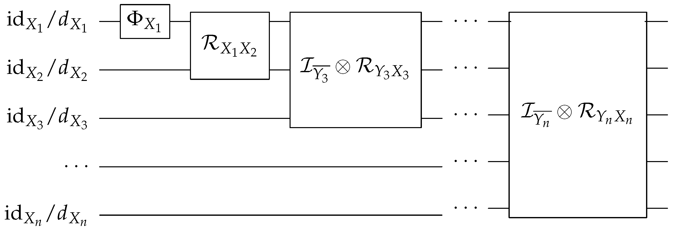
Moreover, given the constructive order, we are also able to make a quantum circuit (c.f. Figure 2) to construct the maximum entropy compatible tree by constructing the first Markov chain ρ X 1 , X 2 , X 3 and then applying the circuits for the recovery maps R of the remaining nodes.    □

4.6. QMT and Chow–Liu Algorithm

Two-body marginals for which all 3-chains form a QMC have another interesting property. It is possible to find the QMT closest, with regards to the quantum relative entropy (the generalization of the Kullback–Leibler divergence [42]), to the unknown density operator. Note that the number of spanning trees over a complete graph is given by Cayley’s formula [43], n n 2 which is exponential on n. To extract the closest QMT, we need to construct a weighted graph (where the nodes are each component of the density operator), and the edges are weighted with the von Neumann mutual information between every two components. The optimal spanning tree, which can be found using the polynomial-time algorithm by Chow–Liu Algorithm 1, gives the support to a QMT. Moreover, this QMT will be the one closest to the unknown state. When the density operators are diagonal, that is, describe a probability distribution, this algorithm coincides with the well-established Chow–Liu algorithm.
Algorithm 1 Chow–Liu Algorithm
  • Input: { C , I C } from a set of RVs X = { X 1 , X n } , where
    • C = { p ( X i , X j ) ; X i X j X } is a set of two-body marginal probability distributions;
    • I C = { I ( X i : X j ) : p ( X i , X j ) C } is the associated set of conditional mutual information.
  • Output: { C T C s.t. H ( p ( X ) | p T ( X ) ) is minimal } , where
    • C T subset of 2-body marginals which associate graph is a tree;
    • p T ( X ) Comp C T .
  • Sort C = { p ( X i , X j ) = p α } α = 1 M 1 2 n ( n 1 ) s.t. I 1 I 2 . . . . I N ;
  • Initialize: C T = α = 0 .
  • Iterate: while a M do
                      if C T p α s.t. G T is a tree
                         then C T = C T { p α } ;
                       α = α + 1 ;
                  return C T
Theorem 5.
If the set of two body marginals C is s.t. every 3-chain is compatible with a QMC then every subtree is a QMT. A QMT that minimizes the quantum relative entropy with respect to the (unknown) given quantum state, is the maximum weighted tree G T C where the weight of each edge is given by the quantum mutual information. Such tree can be obtained efficiently using the (generalized) Chow–Liu learning algorithm [19].
Proof of Theorem 5.
The proof consists in applying Theorem 3 to the main result of Section 6 in the paper [29], that we are going to briefly recall.
Let ρ X be the unknown quantum state that describes best the quantum system for which the bipartite marginals are known (for instance, they have been measured and collected in C ). Moreover, let ρ ˜ C T be the maximum von Neumann entropy d.o. compatible with a subset C T C s.t. G C T is a tree. We refer to ρ ˜ C T as quantum tree. Their relative entropy can be written as
S ρ X | | ρ ˜ C T = S ρ X Tr ρ X log ρ ˜ C T = S ρ ˜ C T S ρ X ,
where we have used condition (i) in Theorem 2 on log ρ ˜ C T .
Therefore, the optimal maximum entropy estimator ρ ˜ is computed over the subtree with minimal von Neumann entropy:
ρ ˜ = argmin C T C max ρ Comp ( C T ) S ρ .
Since the number of possible spanning trees is n n 2 [43], we can not choose the best fitting tree efficiently, in general. However, in the case at hand, we can manipulate Equation (45) and derive subcases for which the computation can be performed efficiently.
Observe that
C T S ρ X i X j i = 1 n deg X i 1 S ρ X i = C T I ρ ( X i , X j ) + i = 1 n S ρ X i ,
and set
Δ S ( ρ ˜ C T ) : = C T S ρ X i X j i = 1 n deg X i 1 S ρ X i S ( ρ ˜ C T ) ,
which is always non-negative. By adding and subtracting the term
C T S ρ X i X j + i = 1 n deg X i 1 S ρ X i
to Equation (45), it assumes the form
S ρ X | | ρ ˜ C T = C T I ρ ( X i , X j ) Δ S ( ρ ˜ C T ) + i = 1 n S ρ X i S ρ X .
By using condition (i) of Theorem 2, we can replace the log term of S ρ ˜ C T of Equation (48) and thus, for a QMT, Δ S ( ρ ˜ C ) = 0 . Moreover, we also have the converse, that is, Δ S ( ρ ˜ C ) = 0 holds only for QMTs. The latter result can be derived by observing that
Δ S ( ρ ˜ C T ) = i = 1 n 2 I ρ ( X l i : V i \ { X l i , ad X l i } | ad X l i ) ,
which, by positivity of quantum conditional mutual information, is 0 iff all the terms in the sum are 0. Then, by Theorem 3, we have Δ S ( ρ ˜ C ) = 0 iff all the 3-chains in C T are QMC.
Therefore, when the provided set of marginals C is s.t. every 3-chain is compatible with a QMC, Δ S ( ρ ˜ C ) = 0 in Equation (50). Therefore, the best tree is the one that maximizes the term
C T I ρ ( X i , X j ) ,
i.e., the maximum weighted spanning sub-tree, where the weights are given by the mutual information between every couple of linked nodes.
This problem is efficiently solved for classical graphs by the Chow–Liu algorithm, which we have here generalized to quantum states, be replacing the Shannon entropy with the von Neumann entropy. □
The general case of efficiently finding the optimal spanning tree which gives the support to a quantum tree remains open. Minimizing the general form of Equation (50) would require the maximization of the quantity C T I ρ ( X i , X j ) + Δ S ( ρ ˜ C T ) with S ( ρ ˜ C T ) > 0 . Already in the tripartite scenario, it is evident that the maximum weighted tree is not a necessarily solution to the problem.
For the sake of completeness, we present the Chow–Liu algorithm in pseudo-code. In its quantum version, the Shannon entropy is replaced by the von Neumann entropy, so as the relative entropy with the quantum relative entropy.

5. Conclusions

In this paper, we addressed the problem of learning the maximum entropy density operator, describing an unknown quantum system on a finite-dimensional Hilbert space, from a set of two-body marginals.
First, we have shown that comparing the entropies of 3-chains—the simplest non-trivial scenario, where two marginals are known in a tripartite quantum system—is QSZK-complete. The result hints that finding the maximum entropy compatible state should be in general not feasible, with a step by step entropy-monotonic procedure.
Then, we determined a subclass of density operators where the addressed problem is in P. Concretely, by observing that the problem at hand naturally abstracts the inference problem for classical probability distribution within graphical models, we ask whether an exact efficient max-entropy learning procedure is limited to classical Markovian systems—the set of constraints is a tree-structured set of mutually commuting density operators. We generalize and extend the classical procedure to a larger subset of density operators, namely two-body marginals compatible with a quantum Markov tree (QMT), whose 3-chains are polynomial-time quantum Markov chains. In addition, for a general set of quantum states whose 3-subchains are quantum Markov chains, we were able to generalize the Chow–Liu algorithm for extracting the optimal QMT. Moreover, we showed that, in the case at hand, the maximum entropy quantum state could be constructed by a polynomial-time quantum circuit.
We stress that the obtained procedures overcome the quantum marginal problem, for which a solution is known in the case of compatibility of the provided set of marginals with a QMT.
Understanding other classes of quantum states for which this problem is tractable (at least in quantum polynomial time) would be a relevant problem. In particular, a further study on the robustness of the procedure can shed some light on the power of quantum machine learning techniques on solving the same problem beyond the Markovian assumption. Indeed, differently from the classical scenario, quantum Markov chains have been proven to be in general distant in trace distance from approximately-Markovian chains—that is, tripartite density operators ρ A B C s.t. I ρ A : B | C ϵ , ϵ > 0 —and the result naturally extends to QMT and many body density operators.

Author Contributions

Conceptualization, S.D.G. and P.M.; Formal analysis, S.D.G.; Funding acquisition, P.M.; Investigation, S.D.G. and P.M.; Methodology, S.D.G. and P.M.; Supervision, P.M.; Writing—original draft, P.M.; Writing—review & editing, S.D.G. and P.M. All authors have read and agreed to the published version of the manuscript.

Funding

This work is supported by Security and Quantum Information Group of Instituto de Telecomunicações, by Programme (COMPETE 2020) of the Portugal 2020 framework [Project Q.DOT with Nr. 039728 (POCI-01-0247-FEDER-039728)] and the Fundação para a Ciência e a Tecnologia (FCT) through national funds, by FEDER, COMPETE 2020, and by Regional Operational Program of Lisbon, under UIDB/50008/2020 (actions QuRUNNER, QUESTS), Project QuantumMining POCI-01-0145-FEDER-031826 and Project PREDICT PTDC/CCI-CIF/29877/2017.

Conflicts of Interest

The authors declare no conflict of interest.

Abbreviations

The following abbreviations are used in this manuscript:
MDPIMultidisciplinary Digital Publishing Institute
DOAJDirectory of open access journals
TLAThree letter acronym
LDlinear dichroism
QSZKQuantum Statistical Zero Knowledge
CPTPCompletely Positive Trace Preserving
QMAQuantum Merlin Arthur
QCMPQuantum Compatible Marginal Problem
MECMPMaximum Entropy Compatible Marginal Problem
BQPBounded-Error Quantum Polynomial Time
(3c)QED(3-chain) Quantum Entropy Difference
QSDQuantum Statistical Difference
QMCQuantum Markov Chain
QMTQuantum Markov Tree

Appendix A. Lemmas for Theorem 1

To perform the proof of Theorem 1, we need the following lemmas.
Lemma A1 (Polarization lemma, Theorem 5 in [25]).
Let α and β satisfy 0 α < β 2 1 . Then, there is a deterministic polynomial-time procedure that, on input ( Q 0 , Q 1 , 1 n ) where Q 0 and Q 1 are quantum circuits, outputs descriptions of quantum circuits ( R 0 , R 1 ) (each having size polynomial in n and in the size of Q 0 and Q 1 ) such that
ρ 0 ρ 1 tr α μ 0 μ 1 tr 2 n , ρ 0 ρ 1 tr β μ 0 μ 1 tr 1 2 n .
The proof of the following lemmas can be found in [38].
Lemma A2 (Joint entropy theorem [38]).
Suppose p i are probabilities, | i are orthogonal states for a system A and ρ i is any set of density operators for another system B. Then,
S i p i | i i | ρ i = H ( p i ) + i p i S ( ρ i ) .
Lemma A3 (Fannes’ inequality [38]).
Suppose ρ and σ are density matrices over a Hilbert space of dimension d. Suppose further that the trace distance between them satisfies t = ρ σ tr 1 / e . Then,
| S ( ρ ) S ( σ ) | t ( ln d ln t ) .
Lemma A4 (Lemma 3.2 in [44]).
Let ρ 0 and ρ 1 be two density matrices, and let ρ = 1 2 ( ρ 0 + ρ 1 ) . If there exists a measurement with outcome 0 or 1 such that making the measurement on ρ b yields the bit b with probability at least p, then
S ( ρ ) 1 2 [ S ( ρ 0 ) + S ( ρ 1 ) ] + ( 1 H ( p ) ) .
In particular, by choosing the right observable we have
Lemma A5 (Theorem 1 in [25]).
Let ρ 0 and ρ 1 be two density matrices, and let ρ = 1 2 ( ρ 0 + ρ 1 ) . Then,
S ( ρ ) 1 2 [ S ( ρ 0 ) + S ( ρ 1 ) ] + ( 1 H ( 1 2 + ρ 0 ρ 1 tr 2 ) ) .

Appendix B. Proof of the Central Lemma 1

The proof of the lemma comes straightforwardly from the following definitions and previously established theorems.
Definition A1.
Let H be a finite dimensional Hilbert space and ρ i B H , i = 1,2, density operators. Their relative entropy is defined as:
S ρ 1 ρ 2 : = T r ρ 1 log ρ 1 log ρ 2 i f s u p p ρ 1 s u p p ρ 2 + o t h e r w i s e .
Originally defined by Umegaki [45]. A relevant property of the quantum relative entropy is its monotonicity under CPTP maps, also known as Uhlmann’s theorem [46].
Theorem A1.
Let H and K be finite dimensional Hilbert spaces, ρ i B H , i = 1,2, density operators with s u p p ρ 1 s u p p ρ 2 . For a CPTP map Φ : B H B K the following inequality holds:
S ρ 1 ρ 2 S Φ ( ρ 1 ) Φ ( ρ 2 ) .
Corollary A1.
The von Neumann entropy is strong sub-additivite:
S ρ A B C ρ A B i d c d C S ρ B C ρ B i d c d C .
Proof of Corollary A1.
Observe that setting in (A6) ρ 1 ρ A B C , ρ 2 ρ A B id C / d C and ϕ ( · ) Tr A · , we obtain which is equivalent to the non-negativity of the quantum conditional mutual information I ρ A : C | B 0 . □
The following two theorems characterize the case of the equality and they will be the core of the proof of Lemma 1.
Theorem A2 (Theorem 2 in [47]).
Let Φ : B H B K be a CPTP map and let ρ i B H , i = 1,2, and ϕ ρ i B K be all invertible density operators. Then, the equality holds in the Uhlmann theorem iff the following equivalent conditions hold:
(i) 
ϕ ϕ ρ 2 i t ϕ ρ 1 i t = ρ 2 i t ρ 1 i t t R ;
(ii) 
ϕ log ϕ ρ 1 log ϕ ρ 2 = log ρ 1 log ρ 2 ;
where ( i i ) is obtained differentiating ( i ) in t = 0.
The adjoint map ϕ ( · ) is understood with respect to the Hilbert–Schmidt inner product.
Theorem A3 (Theorem 5.2 in [35]).
A tripartite state ρ A B C B H A B C is a QMC in the order A-B-C iff I ρ A : C | B = 0 . Furthermore, one can always choose as recovery map the rotated Petz map:
P B B C t ( X ) : = ρ B C 1 + i t 2 ρ B 1 + i t 2 X ρ B 1 i t 2 i d C ρ B C 1 i t 2 , f o r a n y X B ( H B ) , t R .
Proof of Theorem A3 of Lemma 1.
  • (3 ⇒ 1) This implication comes for free from the definition of QMC. Moreover, the map P B B C · is clearly CPTP. The complete positivity indeed comes for free from the Hermitianicity of ρ B id C / d C and ρ B C , then of their square-roots.
  • (1 ⇒ 3) Equation (A8) for t = 0 gives exactly the Petz map in (3), so the implication comes as corollary of Theorem A3.
  • (1 ⇔ 2) This follows from the statement of Theorem A3.
  • (2 ⇔ 4) It comes as corollary of Theorem A2, using the settings in Corollary A1.

Appendix C. Lemmas for Theorem 2 and 3

We need the following Lemmas to derive the proof.
Lemma A6.
Let X = { A , B , C , D } be the labeling of parts of a finite dimensional Hilbert space H and C = { ρ X Y B H X Y , X , Y X } an admissible set of two-body marginals. Assume ρ A B , ρ B C C and ρ ˜ A B C B H A B C : ρ ˜ A B C C o m p ( ρ A B , ρ B C ) such that
I ρ A : C | B = 0 .
(a) 
If the associate graph G C is a chain A-B-C-D (i.e., C = { ρ A B , ρ B C , ρ C D } ) then
ρ ˜ B H : ρ ˜ C o m p C s.t I ρ A : C D | B = 0 iff ρ ˜ B C D B H B C D : ρ ˜ B C D C o m p ( ρ B C , ρ C D ) s . t I ρ B : D | C = 0 .
(b) 
If the associate graph G C is a star centered in B (i.e., C = { ρ A B , ρ B C , ρ B D } )
Mathematics 09 00193 i001
then
ρ ˜ B H : ρ ˜ C o m p C s . t I ρ A : C D | B = 0 iff
(i) 
ρ ˜ C B D C o m p ( ρ B C , ρ B D ) , ρ ˜ B C D B H B C D s.t. I ρ C : D | B = 0 and
(ii) 
ρ ˜ A B D C o m p ( ρ A B , ρ B D ) , ρ ˜ A B D B H A B D s.t. I ρ A : D | B = 0 .
In both the cases, ρ ˜ = a r g m a x ρ C o m p C S ( ρ ) and factorizes over the elements of C via Petz following a constructive ordering for C .
Proof of Lemma A6.
We prove cases (a) and (b) together, but each direction of the equivalence at a time. We notice than one direction follows easily from the chain rule, we start with that direction ( ) Recall the chain rule for quantum conditional mutual information:
I ρ A : X 1 , , X n | B = I ρ A : X 1 | B + I ρ A : X 2 | B X 1 + + + I ρ A : X n | B X 1 , , X n 1
and recall that the conditional mutual information is non negative.
Case (a)
I ρ A B : D | C = I ρ B : D | C + I ρ B : D | A C = 0 I ρ B : D | C = 0
The case (b) is analogous:
I ρ A C : D | B = I ρ A : D | B + I ρ A : D | B C = 0 I ρ A : D | B = 0 I ρ A C : D | B = I ρ C : D | B + I ρ C : D | A B = 0 I ρ C : D | B = 0
( ) (a) To prove the other direction of the statement, we show that there exists a ρ ˜ B H : ρ ˜ Comp ρ ˜ A B C , ρ ˜ B C D and QMC on the order AB-C-D.
By hypothesis and using Lemma 1, the tripartite states can be recovered from two of its two-body marginals using the Petz recovery map:
I ρ A : C | B = 0 iff ρ ˜ A B C = ρ B C 1 2 ρ B 1 2 ρ A B ρ B 1 2 ρ B C 1 2 = ρ A B 1 2 ρ B 1 2 ρ B C ρ B 1 2 ρ A B 1 2 ,
I ρ B : D | C = 0 iff ρ ˜ B C D = ρ B C 1 2 ρ C 1 2 ρ C D ρ C 1 2 ρ B C 1 2 = ρ C D 1 2 ρ C 1 2 ρ B C ρ C 1 2 ρ C D 1 2 .
Using Lemma 2, we check the compatibility of the two marginals with the desired QMC showing that the operator Θ A B C D : = ρ ˜ A B C 1 2 ρ C 1 2 ρ C D 1 2 is normal:
Θ A B C D Θ A B C D = ρ ˜ A B C 1 2 ρ C 1 2 ρ C D ρ C 1 2 ρ ˜ A B C 1 2
  = ρ A B 1 2 ρ B 1 2 ρ B C 1 2 ρ C 1 2 ρ C D ρ C 1 2 ρ B C 1 2 ρ ˜ B C D ρ B 1 2 ρ A B 1 2
  = ρ A B 1 2 ρ B 1 2 ρ C D 1 2 ρ C 1 2 ρ B C ρ C 1 2 ρ C D 1 2 ρ B 1 2 ρ A B 1 2
  = ρ C D 1 2 ρ C 1 2 ρ A B 1 2 ρ B 1 2 ρ B C ρ B 1 2 ρ A B 1 2 ρ ˜ A B C ρ C 1 2 ρ C D 1 2
  = Θ A B C D Θ A B C D .
Equality in Equation (A19) follows for Equation (A16) and Lemma 2. Equality in Equation (A20) follows from permuting density operators in different Hilbert spaces.
(b) Similarly to (a), we show that there exists a ρ ˜ B H : ρ ˜ Comp ρ ˜ A B C , ρ ˜ C B D , ρ ˜ A B D and QMC on the order AC-B-D. Again, using Lemma 1, the tripartite states can be recovered from two of its two-body marginals using the Petz recovery map:
I ρ A : C | B = 0 iff ρ ˜ A B C = ρ B C 1 2 ρ B 1 2 ρ A B ρ B 1 2 ρ B C 1 2 = ρ A B 1 2 ρ B 1 2 ρ B C ρ B 1 2 ρ A B 1 2 ,
I ρ C : D | B = 0 iff ρ ˜ C B D = ρ B C 1 2 ρ B 1 2 ρ B D ρ B 1 2 ρ B C 1 2 = ρ B C 1 2 ρ B 1 2 ρ B D ρ B 1 2 ρ B C 1 2 ,
I ρ A : D | B = 0 iff ρ ˜ A B D = ρ A B 1 2 ρ B 1 2 ρ B D ρ B 1 2 ρ A B 1 2 = ρ A B 1 2 ρ B 1 2 ρ B D ρ B 1 2 ρ A B 1 2 .
First, by using Lemma 2, we check the compatibility of the two marginals ρ B D and ρ A B C with the desired QMC showing that the operator Θ A B C D : = ρ ˜ A B C 1 2 ρ B 1 2 ρ B D 1 2 is normal:
Θ A B C D Θ A B C D = ρ ˜ A B C 1 2 ρ B 1 2 ρ B D ρ B 1 2 ρ ˜ A B C 1 2
  = ρ A B 1 2 ρ B 1 2 ρ B C 1 2 ρ B 1 2 ρ B D ρ B 1 2 ρ B C 1 2 ρ ˜ B C D ρ B 1 2 ρ A B 1 2
  = ρ A B 1 2 ρ B 1 2 ρ B D 1 2 ρ ˜ A B D ρ B 1 2 ρ B C ρ B 1 2 ρ B D 1 2 ρ B 1 2 ρ A B 1 2 ρ ˜ A B D
  = ρ B D 1 2 ρ B 1 2 ρ A B 1 2 ρ B 1 2 ρ B C ρ B 1 2 ρ A B 1 2 ρ ˜ A B C ρ B 1 2 ρ B D 1 2
  = Θ A B C D Θ A B C D .
Moreover, the QMC ρ ˜ = Θ A B C D Θ A B C D is in Comp ρ ˜ A B C , ρ ˜ C B D , ρ ˜ A B D by using Equations (A23)–(A25). □
The previous lemma can be trivially extended to the n-partite scenario, i.e., to an arbitrary chain and a star:
Corollary A2.
Let X = { X 1 , X n } be the labeling set of the parts of a finite dimensional Hilbert space H and C = { ρ X Y B H X Y , X , Y X } a set of two-body marginals on it classically compatible. Assume G C is a star centered in some Y X , i.e., C = { ρ X i Y , i = 1 , , n 1 } then there exists ρ ˜ B H : ρ ˜ C o m p C such that ρ ˜ is a quantum Markov network iff
I ρ X i : X j | Y = 0 i j 1 , , n 1 .
Moreover,
ρ ˜ = a r g m a x ρ Comp C S ( ρ )
and factorizes over the elements of C via Petz following a constructive ordering for C .
Proof of Corollary A2.
The proof follows by adding at each step a node to the setting of Lemma A6 (case b). Shortly, consider the constructive ordering for the graph X = { Y , X 1 , , X n } . Start from graph G 3 , where V 3 Y , X 1 , X 2 , X 3 , clearly in this case we are in the situation of Lemma A6 (b), then:
I ρ ( X 2 : X 1 | Y ) = 0 I ρ ( X 3 : X 1 | Y ) = 0 I ρ ( X 3 : X 1 X 2 | Y ) = 0 .
Observe that the two conditions I ρ ( X 3 : X 1 X 1 | Y ) = 0 and I ρ ( X 2 : X 1 | Y ) = 0 are those required by Theorem 2 s.t. there exists a Petz-factorizable d.o. ρ 3 over G 3 . Next, we add the link X 4 Y to the graph and verify that I ρ ( X 4 : X 1 X 2 X 3 | Y ) = 0 also holds. We need to use again Theorem 2 to construct a Petz-factorizable ρ 4 . This condition follows by applying Lemma A6 (b):
I ρ ( X 4 : X 1 X 2 X 3 | Y ) = 0 iff I ρ ( X 3 : X 1 X 2 | Y ) = 0 and I ρ ( X 4 : X 1 X 2 | Y ) = 0 .
where the first condition is the one we got in the previous step, the second comes from Lemma A6 (b):
I ρ ( X 4 : X 1 X 2 | Y ) = 0 iff I ρ ( X 4 : X 1 | Y ) = 0 a n d I ρ ( X 4 : X 2 | Y ) = 0 .
Then, we keep adding nodes and decomposing the next required condition by Theorem 2. We notice that at each step, i.e., every time we add a node, in order to have a Petz decomposable d.o. on the new graph we have to add to the previous set of 3-chains, all the new 3-chains, i.e., the ones that involve the last added node. □
Lemma A7.
Let ρ B H , where X = { X 1 , , X n } and H = i = 1 n H X i , such that ρ C o m p C with G C a tree (i.e., we work under Assumption 1, and take X 1 < < X n the constructive order). If for some n the following conditions hold
I ρ j X i : Y j ¯ | Y j = 0 , j = 3 , , ,
then, by taking any i and m i i such that
d e g X i | G i = d e g X i | G m i and d e g Y i | G i = d e g Y i | G m i ,
the following conditions also hold
I ρ X i : V r i \ { X i , Y i } | Y i = 0 , r i : i r i m i ,
Proof of Lemma A7.
Take that Equation (A36) with j = ρ r i . By Theorem 2, we know that ρ r i factorizes via Petz over its two-body marginals according to C r i . Then, set
Δ k : = ρ X k Y k 1 2 ρ Y k 1 2 ,
it follows that the factorization via Petz can be written as follows:
ρ r i = Δ r i Δ r i 1 Δ i ρ X 1 X 2 Δ i Δ r i 1 Δ r i ,
where, in general, [ Δ i , Δ j ] 0 . Note that, from the definition of m i it must be the case that [ Δ r i , Δ s ] = 0 s : i s r i . This follows since Equation (A37) imposes that no more nodes are connected to X i and Y i when adding nodes from step i to m i ; and therefore, the additional Δ k ’s operate on different Hilbert spaces. Then, Equation (A40) is to be written as:
ρ k = Δ i Δ r i ρ X 1 X 2 Δ r i Δ i .
Now consider a new, but equivalent, constructive ordering <
X 1 < < X i 1 < X r i < X i + 1 < < X r i 1 < X i ,
obtained from the order < by exchanging r i with i. By using Theorem 2 (ii) with the order < , we get in C r i the condition
I ρ r i X r i : Y r i ¯ | Y r i = 0 .
Which for the usual order < can be stated as:
I ρ X i : V r i \ { X i , Y i } | Y i = 0 .
The latter equality is valid for all r i : i r i m i , since the only property used was the fact that deg X i | G i = deg X i | G r i . □

Appendix D. Number of 3-Chains

Proof of Lemma 3.
We make the proof by counting, for each node X i , how many 3-chains X j X i X k can be formed, and summing all of them afterwards.
For a spanning tree, the lower bound is the number of 3-chains in a n-chain (all nodes have degree 2, with exception of the root and the leaf). In this case, every node is the central node of only one 3-chain, aside for the root and the leaf; thus, # c = n 2 . The upper bound is derived by counting the number of 3-chains in a n-star (there is a root and all the remaining nodes are leaves). The root, say Y, has deg Y = n 1 , and the remaining nodes (enumerate them as X 1 , X n 1 ), have degree one. In this case, consider the first edge X 1 Y , it can be linked through Y to more n-2 nodes, which also gives the number of 3-chains it can be part of. The next edge X 2 Y , it can be connected through Y to n 3 nodes to form n 3 different chains (the chain X 2 Y X 1 is the same as X 1 Y X 2 , which has been already counted for). It is now clear that the number of 3-chains in an n-star is
# c i = k = 2 n ( n k ) = k = 1 n 2 k = 1 2 ( n 1 ) ( n 2 ) .
The number of chains in a n-star is also the number of 3-chains that a node contributes in a complete graph. Then, to obtain the number of 3-chains in a complete graph it is enough to multiply Equation (A45) by the number of nodes, and so # c = n # c i = 1 2 n ( n 1 ) ( n 2 ) .
Another way of obtaining this value consists in using well-known formulas from combinatorial calculus, and observing that the number of 3-chains in a complete graph of n vertices is the number of simple dispositions, i.e., the number of ordered sequences of length 3 without repetitions in a set of n elements, divided by two. The factor 2 comes from the symmetry of the 3-chains; that is, A B C is the same 3-chain as C B A . Then, once again,
# c = 1 2 n ! ( n 3 ) ! = 1 2 n ( n 1 ) ( n 2 )

References

  1. D’Ariano, M.; G Paris, M.G.; Sacchi, M.F. Quantum tomography. Adv. Imaging Electron. Phys. 2003, 128, 206–309. [Google Scholar]
  2. Huber, F.M.; Gühne, O. Characterizing ground and thermal states of few-body Hamiltonians. Phys. Rev. Lett. 2016, 117, 010403. [Google Scholar] [CrossRef] [PubMed]
  3. Cotler, J.; Wilczek, F. Quantum overlapping tomography. Phys. Rev. Lett. 2020, 124, 100401. [Google Scholar] [CrossRef] [PubMed] [Green Version]
  4. Jaynes, E.T. Information theory and statistical mechanics. Phys. Rev. 1957, 106, 620. [Google Scholar] [CrossRef]
  5. Bairey, E.; Arad, I.; Lindner, N.H. Learning a local Hamiltonian from local measurements. Phys. Rev. Lett. 2019, 122, 020504. [Google Scholar] [CrossRef] [PubMed] [Green Version]
  6. Bairey, E.; Guo, C.; Poletti, D.; Lindner, N.H.; Arad, I. Learning the dynamics of open quantum systems from their steady states. New J. Phys. 2020, 22, 032001. [Google Scholar] [CrossRef]
  7. Wiebe, N.; Granade, C.; Ferrie, C.; Cory, D.G. Hamiltonian Learning and Certification Using Quantum Resources. Phys. Rev. Lett. 2014, 112, 190501. [Google Scholar] [CrossRef] [Green Version]
  8. Biamonte, J.; Wittek, P.; Pancotti, N.; Rebentrost, P.; Wiebe, N.; Lloyd, S. Quantum machine learning. Nature 2017, 549, 195. [Google Scholar] [CrossRef]
  9. Anshu, A.; Arunachalam, S.; Kuwahara, T.; Soleimanifar, M. Sample-efficient learning of quantum many-body systems. arXiv 2020, arXiv:2004.07266. [Google Scholar]
  10. Cao, N.; Xie, J.; Zhang, A.; Hou, S.Y.; Zhang, L.; Zeng, B. Supervised learning for quantum maximum entropy estimation. arXiv 2020, arXiv:2005.01540. [Google Scholar]
  11. Klyachko, A.A. Quantum marginal problem and N-representability. In Journal of Physics: Conference Series; IOP Publishing: Bristol, UK, 2006; Volume 36, p. 72. [Google Scholar]
  12. Liu, Y.K. Consistency of local density matrices is QMA-complete. In Approximation, Randomization, and Combinatorial Optimization Algorithms and Techniques; Springer: Berlin/Heidelberg, Germany, 2006; pp. 438–449. [Google Scholar]
  13. Higuchi, A.; Sudbery, A.; Szulc, J. One-qubit reduced states of a pure many-qubit state: Polygon inequalities. Phys. Rev. Lett. 2003, 90, 107902. [Google Scholar] [CrossRef] [PubMed] [Green Version]
  14. Bravyi, S. Requirements for Compatibility between Local and Multipartite Quantum States. Quantum Inf. Comput. 2004, 4, 12–26. [Google Scholar]
  15. Huber, F.M. Quantum States and Their Marginals: From Multipartite Entanglement to Quantum Error-Correcting Codes. Ph.D. Thesis, University of Siegen (DE), Siegen, Germany, 2018. [Google Scholar]
  16. Bishop, C.M. Pattern Recognition and Machine Learning; Springer: Berlin/Heidelberg, Germany, 2006. [Google Scholar]
  17. Dagum, P.; Luby, M. Approximating probabilistic inference in Bayesian belief networks is NP-hard. Artif. Intell. 1993, 60, 141–153. [Google Scholar] [CrossRef] [Green Version]
  18. Valiant, L.G. The complexity of computing the permanent. Theor. Comput. Sci. 1979, 8, 189–201. [Google Scholar] [CrossRef] [Green Version]
  19. Chow, C.K.; Liu, C.N. Approximating discrete probability distributions with dependence trees. IEEE Trans. Inf. Theory 1968, 14, 462–467. [Google Scholar] [CrossRef] [Green Version]
  20. Leifer, M.S.; Spekkens, R.W. Towards a formulation of quantum theory as a causally neutral theory of Bayesian inference. Phys. Rev. A 2013, 88, 052130. [Google Scholar] [CrossRef] [Green Version]
  21. Fitzsimons, J.F.; Jones, J.A.; Vedral, V. Quantum correlations which imply causation. Sci. Rep. 2015, 5, 18281. [Google Scholar] [CrossRef] [Green Version]
  22. Horsman, D.; Heunen, C.; Pusey, M.F.; Barrett, J.; Spekkens, R.W. Can a quantum state over time resemble a quantum state at a single time? Proc. R. Soc. A Math. Phys. Eng. Sci. 2017, 473, 20170395. [Google Scholar] [CrossRef]
  23. Watrous, J. Quantum computational complexity. arXiv 2008, arXiv:0804.3401. [Google Scholar]
  24. Bernstein, E.; Vazirani, U. Quantum complexity theory. Siam J. Comput. 1997, 26, 1411–1473. [Google Scholar] [CrossRef]
  25. Watrous, J. Limits on the power of quantum statistical zero-knowledge. In Proceedings of the 43rd Annual IEEE Symposium on Foundations of Computer Science, Vancouver, BC, Canada, 16–19 November 2002; IEEE: New York, NY, USA, 2002; pp. 459–468. [Google Scholar]
  26. Arora, S.; Barak, B. Computational Complexity: A Modern Approach; Cambridge University Press: Cambridge, UK, 2009. [Google Scholar]
  27. Ben-Aroya, A.; Schwartz, O.; Ta-Shma, A. Quantum Expanders: Motivation and Construction. Theory Comput. 2020, 6, 47–79. [Google Scholar] [CrossRef]
  28. Fawzi, O.; Renner, R. Quantum conditional mutual information and approximate Markov chains. Commun. Math. Phys. 2015, 340, 575–611. [Google Scholar] [CrossRef] [Green Version]
  29. Giorgio, S.D.; Mateus, P.; Mera, B. Recoverability from direct quantum correlations. J. Phys. A Math. Theor. 2020, 53, 185301. [Google Scholar] [CrossRef] [Green Version]
  30. Wang, Y.J. Compatibility among Marginal Densities. Biometrika 2004, 91, 234–239. [Google Scholar] [CrossRef]
  31. De Loera, J.; Onn, S. The Complexity of Three-Way Statistical Tables. Siam J. Comput. 2004, 33, 819–836. [Google Scholar] [CrossRef] [Green Version]
  32. Fritz, T.; Chaves, R. Entropic Inequalities and Marginal Problems. IEEE Trans. Inf. Theory 2013, 59, 803–817. [Google Scholar] [CrossRef] [Green Version]
  33. Watrous, J. Succinct quantum proofs for properties of finite groups. In Proceedings of the 41st Annual Symposium on Foundations of Computer Science, Redondo Beach, CA, USA, 12–14 November 2000; IEEE: New York, NY, USA, 2000; pp. 537–546. [Google Scholar]
  34. Aaronson, S. Quantum computing, postselection, and probabilistic polynomial-time. Proc. R. Soc. A Math. Phys. Eng. Sci. 2005, 461, 3473–3482. [Google Scholar] [CrossRef] [Green Version]
  35. Sutter, D. Approximate Quantum Markov Chains. In Approximate Quantum Markov Chains; Springer International Publishing: Cham, Switzerland, 2018; pp. 75–100. [Google Scholar]
  36. Sutter, D.; Fawzi, O.; Renner, R. Universal recovery map for approximate Markov chains. Proc. R. Soc. A 2016, 472, 20150623. [Google Scholar] [CrossRef]
  37. Choi, M.D. Completely positive linear maps on complex matrices. Linear Algebra Appl. 1975, 10, 285–290. [Google Scholar] [CrossRef] [Green Version]
  38. Nielsen, M.A.; Chuang, I. Quantum Computation and Quantum Information; Cambridge University Press: Cambridge, UK, 2010. [Google Scholar]
  39. Aharonov, D.; Kitaev, A.; Nisan, N. Quantum circuits with mixed states. In Proceedings of the Thirtieth Annual ACM Symposium on Theory of Computing, Berkeley, CA, USA, 28–30 May 1998; pp. 20–30. [Google Scholar]
  40. Löwner, K. Über monotone matrixfunktionen. Math. Z. 1934, 38, 177–216. [Google Scholar] [CrossRef]
  41. Bengtsson, I.; Życzkowski, K. Geometry of Quantum States: An Introduction to Quantum Entanglement; Cambridge University Press: Cambridge, UK, 2006. [Google Scholar]
  42. Cover, T.M.; Thomas, J.A. Elements of Information Theory; John Wiley & Sons: New York, NY, USA, 2012. [Google Scholar]
  43. Cayley, A. A theorem on trees. Quart. J. Math. 1889, 23, 376–378. [Google Scholar]
  44. Ambainis, A.; Nayak, A.; Ta-Shma, A.; Vazirani, U. Dense quantum coding and quantum finite automata. J. Assoc. Comput. Mach. (JACM) 2002, 49, 496–511. [Google Scholar] [CrossRef]
  45. Umegaki, H. Conditional expectation in an operator algebra, IV (entropy and information). In Kodai Mathematical Seminar Reports; Department of Mathematics, Tokyo Institute of Technology: Tokyo, Japan, 1962; Volume 14, pp. 59–85. [Google Scholar]
  46. Uhlmann, A. Relative entropy and the Wigner-Yanase-Dyson-Lieb concavity in an interpolation theory. Commun. Math. Phys. 1977, 54, 21–32. [Google Scholar] [CrossRef]
  47. Petz, D. Monotonicity of quantum relative entropy revisited. Rev. Math. Phys. 2003, 15, 79–91. [Google Scholar] [CrossRef] [Green Version]
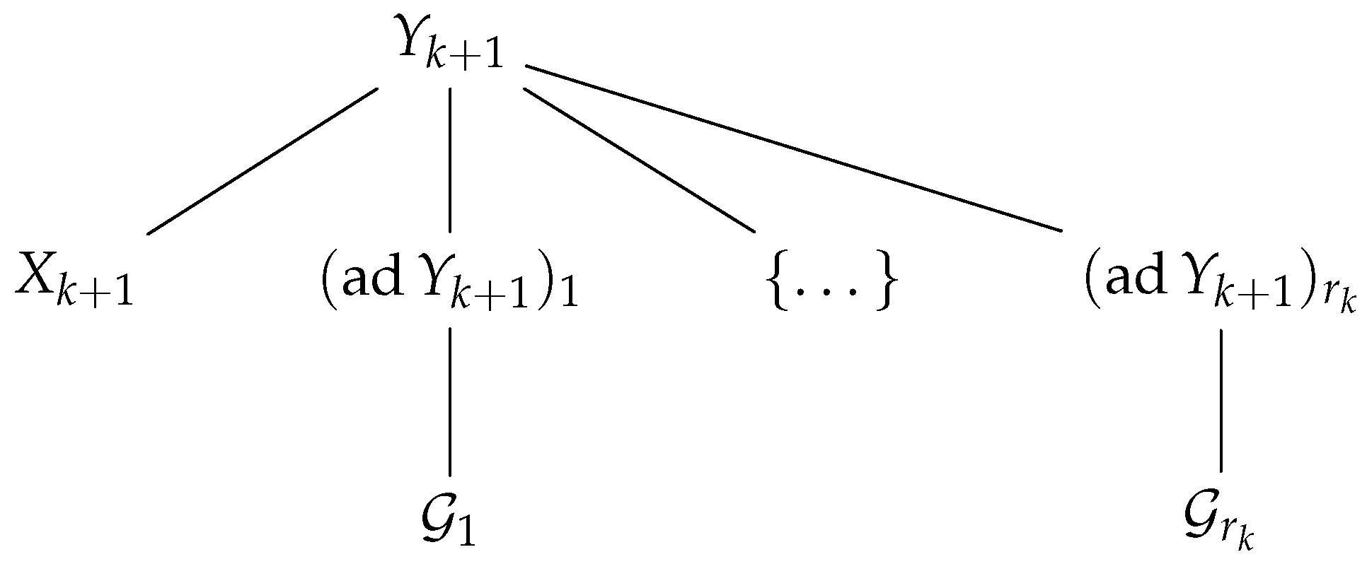
Figure 1. The associate graph G k + 1 : can be seen as a star centered in Y k + 1 , where every branch is an adjacent of Y k + 1 in V k , plus the link to X k + 1 . G i indicates the rest of the graph (a tree) that is connected to the i-th adjacent ( ad Y k + 1 ) i . The number of adjacent nodes to Y k + 1 in G k + 1 is r k + 1 by adding X k + 1 to other r k nodes in G k .
Mathematics 09 00193 g001
Figure 2. Quantum circuit that outputs the optimal quantum Markov trees (QMT). Note that the k-th block I Y k ¯ R Y k X k operates only over two components X k and Y k , for all k = 3 n .
Mathematics 09 00193 g002
Publisher’s Note: MDPI stays neutral with regard to jurisdictional claims in published maps and institutional affiliations.