Series Solutions of High-Dimensional Fractional Differential Equations

Abstract

In the present paper, the series solutions and the approximate solutions of the time–space fractional differential equations are obtained using two different analytical methods. One is the homotopy perturbation Sumudu transform method (HPSTM), and another is the variational iteration Laplace transform method (VILTM). It is observed that the approximate solutions are very close to the exact solutions. The solutions obtained are very useful and significant to analyze many phenomena, and the solutions have not been reported in previous literature. The salient feature of this work is the graphical presentations of the third approximate solutions for different values of order $\alpha$.

1. Introduction

The fractional derivative has a long history which is as old as the integer derivative and was first mentioned in a letter from Leibniz to L’Hospital in 1695 [1]. Presently, this subject is widely applied in plasma physics, fluid dynamics, solid-state physics, engineering, economics, medicine, financial market, non-Newtonian mechanics, automatic control theory, chemical physics and so on (see [2,3,4,5,6,7,8], for example). In particular, the authors obtained the existence and uniqueness of the solution of fractional epidemiological model for computer viruses [6] and fractional SIR epidemic model of childhood disease [7], respectively. The reason it is widely used in science and engineering community is that fractional derivative is not a local operator. That means the next state of an equation depends not only on its current state but also on all its historical states. This strong memory effects shows that fractional derivative is very important to represent the treatment and to manage the malaria disease and other kinds of problems [7]. However, many definitions of fractional integral and fractional derivative have been proposed without a uniform one, for instance, Riemann–Liouville fractional integral, Caputo fractional derivative, Weyl fractional derivative [9], Caputo–Fabrizio fractional derivative [6], Atanagana–Baleanu fractional derivative [7] and so on. The most commonly used definitions are Riemann–Liouville integral and Caputo derivative.

For general nonlinear equations, it is difficult to derive exact solutions. If they are not available, the obtaining of the series solutions or the numerical solutions may be crucial, because they can interpret many physical phenomena and are useful for physicists. Therefore, the exact solutions can be replaced by the approximate solutions within a certain scale. There are several approximation methods for deriving series solutions of fractional differential equations, including the Adomian decomposition method [10,11], the homotopy analysis method [12,13,14], the variational iteration method [15,16], the homotopy perturbation method [17,18], the Exp-function method [19,20] and the Elzaki projected differential transform method [21] and so on.

In ref. [22], the homotopy perturbation Sumudu transform method was proposed, which was an elegant combination of Sumudu transform and homotopy perturbation method, and it is a powerful mathematical method for solving fractional differential equations. In ref. [23], the authors extended the HPSTM to the time fractional differential equation. In this work, we apply this method to general time–space fractional differential equations. Comparing the HPSTM with other classical numerical methods, we know that the HPSTM not only reduce the volume of computational work but also maintain a high accuracy of the results. At the same time, the HPSTM does not need over restrictive assumption or linearization.

In ref. [24], the authors proposed an analytical method, called the variational iteration Laplace transform method. In this method, Laplace transform can overcome principle drawbacks in applications of the variational iteration method to fractional equations. The VILTM was also investigated by many authors to handle time fractional equations arising in science and engineering [25,26]. In ref. [27], the authors chose Lagrange multiplier as $-1$ to obtain analytical solutions of fractional wave-like equations. In the VILTM, the main problem is how to determine the Lagrange multiplier. Until now, there is no effective method to identify the Lagrange multiplier. In this work, using the Laplace transform, we can easily derive new variational iteration formula and Lagrange multiplier without tedious calculations.

The rest of the paper is organized as follows. In Section 2, we introduce some basic ideas of fractional calculus, the Sumudu transform and the Laplace transform. In Section 3, we illustrate the concrete steps of the HPSTM, and provide the condition for convergence and error estimates of the method. In Section 4, we illustrate the concrete steps of the VILTM, and provide the condition for convergence and error estimates of the method. In Section 5, we apply the HPSTM and the VILTM to obtain approximation solutions of fractional equations with initial values. We also include some numerical results to illustrate our results. Throughout the paper, the equations with fractional-order derivatives in the Caputo sense are considered.

2. Preliminaries

Definition 1

([9]). A real function f: ${\mathbb{R}}^{+}\to \mathbb{R}$ belongs to ${\mathbb{C}}_{\mu }$, $\mu \in \mathbb{R}$, if there exists a real number $k>\mu$ such that $f(x)=x^{k}g(x)$, where $g(x)\in C[0,+\infty )$, and it is said to be in the space ${\mathbb{C}}_{\mu }^m$ if $f^{(m)}\in {\mathbb{C}}_{\mu },m\in \mathbb{N}$.

Definition 2

([9]). The Riemann–Liouville fractional integral of order $\alpha ⩾0$ of a function $f\in {\mathbb{C}}_{\mu }$ is defined as follows:

$${\mathrm{I}}^{\alpha }f(x):=\left\{\begin{array}{cc}\frac{1}{\Gamma (\alpha )}{\int }_0^x{(x-\tau )}^{\alpha -1}f(\tau )\mathrm{d}\tau ,\hfill & \alpha >0,x>0,\hfill \\ f(x),\hfill & \alpha =0,\hfill \end{array}\right.$$

where $\mu ⩾-1$, Γ is the Gamma function.

Definition 3

([9]). The Caputo fractional derivative operator of order $\alpha >0$ of $f\in {\mathbb{C}}_{\mu }^n(\mu ⩾-1,n\in \mathbb{N})$ is defined as follows:

$$\begin{array}{c}\hfill {\mathrm{D}}^{\alpha }f(x):=\left\{\begin{array}{cc}\frac{1}{\Gamma (n-\alpha )}{\int }_0^x{(x-\tau )}^{n-\alpha -1}{f}^{(n)}(\tau )\mathrm{d}\tau ,\hfill & n-1<\alpha <n,x>0,\hfill \\ f^{(n)}(x),\hfill & \alpha =n.\hfill \end{array}\right.\end{array}$$

Consider $f(x,t)$ as a function of t, if it belongs to ${\mathbb{C}}_{\mu }^n(\mu ⩾-1,n\in \mathbb{N})$, then we have the following definition for time fractional derivative.

Definition 4

([9]). The Caputo time fractional derivative operator of order $\alpha >0$ of $f(x,t)$ is defined as follows:

$$\begin{array}{c}\hfill {\mathrm{D}}_t^{\alpha }f(x,t):=\left\{\begin{array}{cc}\frac{1}{\Gamma (n-\alpha )}{\int }_0^t{(t-\tau )}^{n-\alpha -1}\frac{{\partial }^{n}f(x,\tau )}{\partial {\tau }^n}\mathrm{d}\tau ,\hfill & n-1<\alpha <n,t>0,\hfill \\ \frac{{\partial }^{n}f(x,t)}{\partial t^n},\hfill & \alpha =n.\hfill \end{array}\right.\end{array}$$

Consider $f(x,t)$ as a function of x, if it belongs to ${\mathbb{C}}_{\mu }^n(\mu ⩾-1,n\in \mathbb{N})$, then we have the following definition for space fractional derivative.

Definition 5

([9]). The Caputo space fractional derivative operator of order $\beta >0$ of $f(x,t)$ is defined as follows:

$$\begin{array}{c}\hfill {\mathrm{D}}_x^{\beta }f(x,t):=\left\{\begin{array}{cc}\frac{1}{\Gamma (n-\beta )}{\int }_0^x{(x-\tau )}^{n-\beta -1}\frac{{\partial }^{n}f(\tau ,t)}{\partial {\tau }^n}\mathrm{d}\tau ,\hfill & n-1<\beta <n,x>0,\hfill \\ \frac{{\partial }^{n}f(x,t)}{\partial x^n},\hfill & \beta =n.\hfill \end{array}\right.\end{array}$$

Definition 6

([28]). The Sumudu transform, is defined over the set of function

$$A=\left\{f(t):\exists M,{\tau }_1,{\tau }_2>0,s.t.\left|f(t)\right|<M{e}^{\frac{\left|t\right|}{{\tau }_j}},\mathrm{if}t\in {(-1)}^j\times [0,+\infty )\right\}$$

by the following formula:

$$S[f(t)](u)={\int }_0^{\infty }f(ut)e^{-t}\mathrm{d}t,u\in (-{\tau }_1,{\tau }_2).$$

Definition 7

([25]). The Laplace transform, is defined over the set of function

$$A=\left\{f(t)\in C[0,+\infty ):\exists M>0anda\in \mathbb{R},s.t.\left|f(t)\right|\le M{e}^{at}\right\}$$

by the following formula:

$$L[f(t)](s)={\int }_0^{\infty }f(t)e^{-st}\mathrm{d}t,s>a.$$

Property 1

([29,30]). (i) The Sumudu transform satisfies linear property, i.e.,

$$\begin{array}{c}\hfill S[af(t)+bh(t)]=aS[f(t)]+bS[h(t)],\end{array}$$

where $a,$ b are constants.

(ii)

$$\begin{array}{c}\hfill S[t^{\alpha }]=u^{\alpha }\Gamma (\alpha +1),\alpha >0.\end{array}$$

Property 2

([25]). (i) The Laplace transform satisfies linear property, i.e.,

$$\begin{array}{c}\hfill L[af(t)+bh(t)]=aL[f(t)]+bL[h(t)],\end{array}$$

where $a,$ b are constants.

(ii)

$$\begin{array}{c}\hfill L[t^{\alpha }]=s^{-\alpha -1}\Gamma (\alpha +1),\alpha >0.\end{array}$$

Lemma 1

([29,30]). The Sumudu transform of the Caputo fractional derivative is

$$\begin{array}{c}\hfill S[{\mathrm{D}}_t^{\alpha }f(t)]=u^{-\alpha }S[f(t)]-\sum _{k=0}^m{u}^{-\alpha +k}{f}^{(k)}(0),m<\alpha \le m+1,m\in \mathbb{N}.\end{array}$$

(1)

Lemma 2

([25]). The Laplace transform of the Caputo fractional derivative is

$$\begin{array}{c}\hfill L[{\mathrm{D}}_t^{\alpha }f(t)]=s^{\alpha }L[f(t)]-\sum _{k=0}^m{s}^{\alpha -k-1}{f}^{(k)}(0),m<\alpha \le m+1,m\in \mathbb{N}.\end{array}$$

(2)

3. Homotopy Perturbation Sumudu Transform Method

In this section, we extend the algorithm of HPSTM [22] to the general fractional nonhomogeneous differential equation in ${\mathbb{R}}^3$

$${\mathrm{D}}_t^{\alpha }U(x,y,z,t)+\mathcal{R}U(x,y,z,t)+\mathcal{N}U(x,y,z,t)=g(x,y,z,t)$$

(3)

with the initial condition

$$U(x,y,z,0)=f(x,y,z),$$

(4)

where $\alpha \in (0,1]$, $(x,y,z)\in {\mathbb{R}}^3$, $t\in [0,\infty )$, $\mathcal{R}$ and $\mathcal{N}$ represent the linear and the nonlinear differential operator, respectively, $g(x,y,z,t)$ is the source term.

Applying the Sumudu transform to both sides of (3), we obtain

$$S[{\mathrm{D}}_t^{\alpha }U(x,y,z,t)]+S[\mathcal{R}U(x,y,z,t)]+S[\mathcal{N}U(x,y,z,t)]=S[g(x,y,z,t)].$$

According to the property (1), we have

$$S[U(x,y,z,t)]=f(x,y,z)-u^{\alpha }S[\mathcal{R}U(x,y,z,t)+\mathcal{N}U(x,y,z,t)-g(x,y,z,t)].$$

(5)

Furthermore, applying the inverse Sumudu transform $S^{-1}$ to both sides of (5), we can obtain

$$U(x,y,z,t)=M(x,y,z,t)-S^{-1}[u^{\alpha }S[\mathcal{R}U(x,y,z,t)+\mathcal{N}U(x,y,z,t)]],$$

where $M(x,y,z,t)$ represents the term arising from the initial condition and the source term, i.e.,

$$M(x,y,z,t)=f(x,y,z)+S^{-1}[u^{\alpha }S[g(x,y,z,t)]].$$

Now we construct the homotopy perturbation equation as follows

$$U(x,y,z,t)=M(x,y,z,t)-p\times S^{-1}[u^{\alpha }S[\mathcal{R}U(x,y,z,t)+\mathcal{N}U(x,y,z,t)]],p\in [0,1].$$

(6)

According to standard homotopy perturbation method, the solution of (6) is

$$\begin{array}{cc}\hfill U(x,y,z,t)& =\sum _{n=0}^{\infty }{p}^n{U}_n(x,y,z,t),\hfill \end{array}$$

(7)

and the nonlinear term $\mathcal{N}U(x,y,z,t)$ can be decomposed into

$$\begin{array}{cc}\hfill \mathcal{N}U(x,y,z,t)& =\sum _{n=0}^{\infty }{p}^n{H}_n(U),\hfill \end{array}$$

(8)

where $H_n(U)$ are Adomian polynomials

$$\begin{array}{cc}\hfill H_n(U)& =\frac{1}{n!}\frac{{\partial }^n}{\partial p^n}\left(\mathcal{N}\left(\sum _{k=0}^{\infty }{p}^k{U}_k\right)\right){|}_{p=0}.\hfill \end{array}$$

Now, substituting (7) and (8) into (6), we can obtain

$$\sum _{n=0}^{\infty }{p}^n{U}_n(x,y,z,t)=M(x,y,z,t)-p\times S^{-1}\left[u^{\alpha }S\left[\mathcal{R}\left(\sum _{n=0}^{\infty }{p}^n{U}_n(x,y,z,t)\right)+\sum _{n=0}^{\infty }{p}^n{H}_n(U)\right]\right].$$

(9)

Comparing the coefficients of same powers of p, we obtain the following recurrence equations

$$\begin{array}{cc}\hfill p^0:U_0(x,y,z,t)=& M(x,y,z,t),\hfill \\ \hfill p^n:U_n(x,y,z,t)=& -S^{-1}\left[u^{\alpha }S[\mathcal{R}{U}_{n-1}(x,y,z,t)+H_{n-1}(U)]\right],n=1,2,\cdots .\hfill \end{array}$$

According to the HPM, we assume that the solution of (4)–(6) can be written as

$$V(x,y,z,t)=\underset{n\to \infty }{lim}\left(U_0+U_{1}p+U_2{p}^2+\cdots +U_n{p}^n\right).$$

(10)

Thus, the solution of (3) and (4) is

$$U(x,y,z,t)=\underset{p\to 1}{lim}V(x,y,z,t)=\underset{n\to \infty }{lim}\left(U_0+U_1+U_2+\cdots +U_n\right).$$

The nonlinear differential operator $\mathcal{N}$ determines the convergence of series (10). Since the parameter p may be relatively large (we can take $p\to 1$), the derivatives of the nonlinear part must be chosen sufficiently small. Actually, the series is convergent for most cases [17]. Moreover, there are many references discussing the convergence of series approximate solutions by the homotopy perturbation method, one can see [31] for example.

In the following, we will provide a condition for the convergence of the HPSTM. To do this, we first define an operator $\mathcal{T}:X\to X$ by

$$\begin{array}{c}\hfill \mathcal{T}[v(x,y,z,t)]=S^{-1}[u^{\alpha }S[v(x,y,z,t)]],\end{array}$$

where $X=\{v(x,y,z,t)$: v is continuous on $(x,y,z,t)\in {\mathbb{R}}^3\times [0,\infty )\}$ is a Banach space with norm $\left|\right|v\left|\right|$. Since S is a linear operator, we know that $\mathcal{T}$ is a linear operator. The norm of a linear operator $\mathcal{T}$ is defined by

$$\left|\right|\mathcal{T}\left|\right|=sup\{|\left|\mathcal{T}v\right||,|\left|v\right||\le 1\}.$$

Then we have the following theorem for the convergence of the HPSTM.

Theorem 1.

Suppose that the linear operators $\mathcal{T}$ and $\mathcal{R}$ satisfy $\left|\right|\mathcal{TR}\left|\right|<1$, and the nonlinear operator $\mathcal{N}$ satisfies

$$\left|\right|\mathcal{TN}u-\mathcal{TN}v\left|\right|\le \gamma \left|\right|u-v\left|\right|,u,v\in X,$$

for some constant $0<\gamma <1-\left|\right|\mathcal{TR}\left|\right|$. Then the series solution ${\sum }_{k=0}^{\infty }{U}_k(x,y,z,t)$ is convergent.

Proof. 

The recurrence equations become

$$\begin{array}{c}\hfill U_n(x,y,z,t)=-\mathcal{TR}{U}_{n-1}(x,y,z,t)-\mathcal{T}{H}_{n-1}(U),n=1,2,\cdots .\end{array}$$

Suppose that $\{S_n(x,y,z,t)\}$ is the sequence of partial sums of the series solution, i.e.,

$$S_n(x,y,z,t)=\sum _{k=0}^n{U}_k(x,y,z,t),n=1,2,\cdots .$$

In ref. [32], it was pointed out that the Adomian polynomials $H_n(U)$ only depend on $U_0,\cdots ,U_n$, and thus we can calculate $H_n(U)$ in an explicit manner by the following relation

$$\begin{array}{c}\hfill \mathcal{N}\left(\sum _{k=0}^n{p}^k{U}_k(x,y,z,t)\right)=\sum _{k=0}^n{p}^k{H}_k(U).\end{array}$$

Let $p=1$, we have

$$\begin{array}{c}\hfill \mathcal{N}{S}_n(x,y,z,t)=\sum _{k=0}^n{H}_k(U).\end{array}$$

Hence, we have

$$\begin{array}{c}\hfill \mathcal{T}{H}_n(U)=\mathcal{T}\mathcal{N}{S}_n(x,y,z,t)-\mathcal{T}\mathcal{N}{S}_{n-1}(x,y,z,t).\end{array}$$

For any $n>0$, we have

$$\begin{array}{cc}\hfill & \left|\right|S_{n+1}(x,y,z,t)-S_n(x,y,z,t)\left|\right|=\left|\right|\mathcal{TR}{U}_n(x,y,z,t)+\mathcal{T}{H}_n(U)\left|\right|\hfill \\ \hfill \le & \left|\right|\mathcal{TR}{U}_n(x,y,z,t)\left|\right|+\left|\right|\mathcal{T}\mathcal{N}{S}_n(x,y,z,t)-\mathcal{T}\mathcal{N}{S}_{n-1}(x,y,z,t)\left|\right|\hfill \\ \hfill \le & (|\left|\mathcal{TR}\right||+\gamma )||U_n(x,y,z,t)\left|\right|\le \cdots \le {(|\left|\mathcal{TR}\right||+\gamma )}^{n+1}\left|\right|U_0(x,y,z,t)\left|\right|.\hfill \end{array}$$

For any $m>n>0$, we have

$$\begin{array}{c}\hfill \begin{array}{cc}\hfill & \left|\right|S_m(x,y,z,t)-S_n(x,y,z,t)\left|\right|\hfill \\ \hfill \le & \left|\right|S_m(x,y,z,t)-S_{m-1}(x,y,z,t)\left|\right|+\cdots +\left|\right|S_{n+1}(x,y,z,t)-S_n(x,y,z,t)\left|\right|\hfill \\ \hfill \le & \sum _{k=n+1}^m{(|\left|\mathcal{TR}\right||+\gamma )}^k\left|\right|U_0(x,y,z,t)\left|\right|<\frac{{(|\left|\mathcal{TR}\right||+\gamma )}^{n+1}}{1-(|\left|\mathcal{TR}\right||+\gamma )}\left|\right|U_0(x,y,z,t)\left|\right|.\hfill \end{array}\end{array}$$

(11)

Since $0<\left|\right|\mathcal{TR}\left|\right|+\gamma <1$, we know that $\{S_n(x,y,z,t)\}$ is a Cauchy sequence in Banach space X, so it converges, and we have

$$\begin{array}{c}\hfill U(x,y,z,t)=\underset{n\to \infty }{lim}\sum _{k=0}^n{U}_k(x,y,z,t).\end{array}$$

Let $m\to \infty$ in inequality (11), we have the following error estimates

$$\begin{array}{c}\hfill \left|\right|U(x,y,z,t)-S_n(x,y,z,t)\left|\right|<\frac{{(|\left|\mathcal{TR}\right||+\gamma )}^{n+1}}{1-(|\left|\mathcal{TR}\right||+\gamma )}\left|\right|U_0(x,y,z,t)\left|\right|.\end{array}$$

The proof is completed. □

Remark 1.

Comparing the HPSTM with other classical methods, we know that the homotopy series solutions for fractional equations can be constructed without using any overstrict assumption.

4. Variational Iteration Laplace Transform Method

In this section, we introduce the algorithm of VILTM [24,25,26] for the general fractional nonhomogeneous differential Equation (3) with the initial condition (4).

Applying the Laplace transform L to both sides of (3), then the iteration formula of (3) becomes

$$\begin{array}{c}\hfill \begin{array}{cc}\hfill U_{n+1}(x,y,z,s)=& U_n(x,y,z,s)+\lambda (s)[s^{\alpha }{U}_n(x,y,z,s)\hfill \\ & -f(x,y,z)s^{\alpha -1}+L[\mathcal{R}[U_n(x,y,z,t)]+\mathcal{N}[U_n(x,y,z,t)]-g(x,y,z,t)]],\hfill \end{array}\end{array}$$

(12)

where $U_n$ is the n-th order approximate solution. Considering $L(\mathcal{R}[U_n]+\mathcal{N}[U_n])$ as restricted term, the Lagrange multiplier can be identified as

$$\lambda =-\frac{1}{s^{\alpha }}.$$

Applying the inverse Laplace transform $L^{-1}$ to both sides of (12), we obtain

$$\begin{array}{c}\hfill \begin{array}{cc}\hfill U_{n+1}(x,y,z,t)=& U_n(x,y,z,t)-L^{-1}[s^{-\alpha }[s^{\alpha }{U}_n(x,y,z,s)\hfill \\ & -f(x,y,z)s^{\alpha -1}+L[\mathcal{R}[U_n(x,y,z,t)]+\mathcal{N}[U_n(x,y,z,t)]-g(x,y,z)]]]\hfill \\ \hfill =& U_0(x,y,z,t)-L^{-1}[s^{-\alpha }L[\mathcal{R}[U_n(x,y,z,t)]+\mathcal{N}[U_n(x,y,z,t)]]],\hfill \end{array}\end{array}$$

(13)

where the initial iteration value $U_0(x,y,z,t)$ can be determined as

$$\begin{array}{c}\hfill U_0(x,y,z,t)=f(x,y,z)+L^{-1}[s^{-\alpha }L[g(x,y,z,t)]].\end{array}$$

Finally, the approximation solution is

$$\begin{array}{c}\hfill U(x,y,z,t)=\underset{n\to \infty }{lim}{U}_n(x,y,z,t).\end{array}$$

There are many references discussing the convergence of approximate solutions by variational iteration method, one can see [33] for example. In ref. [33], based on the sufficient condition that guarantees the existence of a unique solution, the authors proved that the series solution is convergence.

The following theorem provides the convergence for the VILTM.

Theorem 2.

Suppose that the conditions of Theorem 1 are satisfied. Then the approximate solution $U_n(x,y,z,t)$ is convergent.

Proof. 

The Sumudu transform and the Laplace transform exhibit a duality relation expressed as follows:

$$S[f(t)](\frac{1}{s})=sL[f(t)](s),L[f(t)](\frac{1}{u})=uS[f(t)](u),\mathrm{for}s,u>0.$$

By this duality relation, we can prove that

$$S^{-1}[u^{\alpha }S[f(t)]]=L^{-1}[s^{-\alpha }L[f(t)]].$$

Then we have

$$\begin{array}{c}\hfill L^{-1}[s^{-\alpha }L[u(x,y,z,t)]]=\mathcal{T}[u(x,y,z,t)].\end{array}$$

Hence, the iteration formula becomes

$$\begin{array}{c}\hfill U_{n+1}(x,y,z,t)=U_0(x,y,z,t)-\mathcal{TR}[U_n(x,y,z,t)]-\mathcal{TN}[U_n(x,y,z,t)].\end{array}$$

For any $n>0$, we have

$$\begin{array}{cc}\hfill & \left|\right|U_{n+1}(x,y,z,t)-U_n(x,y,z,t)\left|\right|\hfill \\ \hfill \le & \left|\right|\mathcal{TR}{U}_n(x,y,z,t)-\mathcal{TR}{U}_{n-1}(x,y,z,t)\left|\right|+\left|\right|\mathcal{TN}{U}_n(x,y,z,t)-\mathcal{TN}{U}_{n-1}(x,y,z,t)\left|\right|\hfill \\ \hfill \le & (|\left|\mathcal{TR}\right||+\gamma )||U_n(x,y,z,t)-U_{n-1}(x,y,z,t)\left|\right|\hfill \\ \hfill \le & \cdots \le {(|\left|\mathcal{TR}\right||+\gamma )}^n\left|\right|U_1(x,y,z,t)-U_0(x,y,z,t)\left|\right|\hfill \\ \hfill =& {(|\left|\mathcal{TR}\right||+\gamma )}^n\left|\right|\mathcal{TR}{U}_0(x,y,z,t)+\mathcal{TN}{U}_0(x,y,z,t)\left|\right|.\hfill \end{array}$$

For any $m>n>0$, we have

$$\begin{array}{c}\hfill \begin{array}{cc}\hfill & \left|\right|U_m(x,y,z,t)-U_n(x,y,z,t)\left|\right|\hfill \\ \hfill \le & \left|\right|U_m(x,y,z,t)-U_{m-1}(x,y,z,t)\left|\right|+\cdots +\left|\right|U_{n+1}(x,y,z,t)-U_n(x,y,z,t)\left|\right|\hfill \\ \hfill \le & \sum _{k=n}^{m-1}{(|\left|\mathcal{TR}\right||+\gamma )}^k\left|\right|\mathcal{TR}{U}_0(x,y,z,t)+\mathcal{TN}{U}_0(x,y,z,t)\left|\right|\hfill \\ \hfill <& \frac{{(|\left|\mathcal{TR}\right||+\gamma )}^n}{1-(|\left|\mathcal{TR}\right||+\gamma )}\left|\right|\mathcal{TR}{U}_0(x,y,z,t)+\mathcal{TN}{U}_0(x,y,z,t)\left|\right|.\hfill \end{array}\end{array}$$

(14)

Since $0<\left|\right|\mathcal{TR}\left|\right|+\gamma <1$, we know that $\{U_n(x,y,z,t)\}$ is a Cauchy sequence in Banach space X, so it converges, and we have

$$\begin{array}{c}\hfill U(x,y,z,t)=\underset{n\to \infty }{lim}{U}_n(x,y,z,t).\end{array}$$

Let $m\to \infty$ in inequality (14), we have the following error estimates

$$\begin{array}{c}\hfill \left|\right|U(x,y,z,t)-U_n(x,y,z,t)\left|\right|<\frac{{(|\left|\mathcal{TR}\right||+\gamma )}^n}{1-(|\left|\mathcal{TR}\right||+\gamma )}\left|\right|\mathcal{TR}{U}_0(x,y,z,t)+\mathcal{TN}{U}_0(x,y,z,t)\left|\right|.\end{array}$$

The proof is completed. □

Remark 2.

The VILTM is easy to apply, which simplifies the applications of variational iteration method to fractional differential equations, and improves the convergence of iteration.

5. Applications of HPSTM and VILTM to Fractional Differential Equations

5.1. The One-Dimensional Time–Space Fractional KdV Equation

The nonlinear KdV equation is an important mathematical model in physics and engineering. The fractional KdV equation has been applied to model a wide range of physical phenomena, such as internal waves in coastal waters, waves in plasma physics, magma flow and conduit waves, flow in blood vessels, boundary layer behavior and so on. In ref. [34], the author introduced a fractional KdV equation with initial conditions, and the explicit numerical solutions are derived by the Adomian decomposition method. In this section, we employ the HPSTM and the VILTM to obtain the series solutions of the following KdV equation, namely

$$\begin{array}{c}\hfill {\mathrm{D}}_t^{\alpha }U(x,t)={\mathrm{D}}_x^{3}U(x,t)+U(x,t){\mathrm{D}}_x^{\beta }U(x,t)\end{array}$$

(15)

with the initial condition

$$U(x,0)=x^2,$$

where $0<\alpha ,\beta \le 1,(x,t)\in \mathbb{R}\times [0,\infty )$.

5.1.1. Homotopy Perturbation Sumudu Transform Method

Applying the Sumudu transform to both sides of (15) and taking into account the initial condition, we have

$$\begin{array}{c}\hfill S[U(x,t)]=x^2+u^{\alpha }S[{\mathrm{D}}_x^{3}U(x,t)+U(x,t){\mathrm{D}}_x^{\beta }U(x,t)].\end{array}$$

(16)

Then the inverse Sumudu transform of (16) implies that

$$\begin{array}{c}\hfill U(x,t)=x^2+S^{-1}[u^{\alpha }S[{\mathrm{D}}_x^{3}U(x,t)+U(x,t){\mathrm{D}}_x^{\beta }U(x,t)]].\end{array}$$

(17)

Now we apply the homotopy perturbation method to obtain the following equation

$$\begin{array}{c}\hfill \sum _{n=0}^{\infty }{p}^n{U}_n(x,t)=x^2+p\times S^{-1}\left[u^{\alpha }S\left[{\mathrm{D}}_x^3\left(\sum _{n=0}^{\infty }{p}^n{U}_n(x,t)\right)+\sum _{n=0}^{\infty }{p}^n{H}_n^U(x,t)\right]\right],\end{array}$$

where the nonlinear terms $H_n^U(x,t)$ are Adomian polynomials, which are given by

$$\begin{array}{cc}\hfill \sum _{n=0}^{\infty }{p}^n{H}_n^U(x,t)& =U(x,t){\mathrm{D}}_x^{\beta }U(x,t).\hfill \end{array}$$

Set

$$\begin{array}{c}\hfill U_n(x,t):={\tilde{U}}_n(x)\frac{t^{n\alpha }}{\Gamma (n\alpha +1)},\end{array}$$

then

$$\begin{array}{cc}\hfill H_n^U(x,t)=& \sum _{i=0}^n{\tilde{U}}_i(x){\mathrm{D}}_x^{\beta }{\tilde{U}}_{n-i}(x)\frac{t^{n\alpha }}{\Gamma (i\alpha +1)\Gamma ((n-i)\alpha +1)}.\hfill \end{array}$$

Comparing the coefficients with identical powers in p, we have

$$\begin{array}{cc}\hfill p^0:U_0(x,t)& ={\tilde{U}}_0(x)=x^2,\hfill \\ \hfill p^1:U_1(x,t)& =S^{-1}[u^{\alpha }S[{\mathrm{D}}_x^3{U}_0(x,t)+H_0^U(x,t)]]\hfill \\ \hfill & =S^{-1}[u^{\alpha }S[{\mathrm{D}}_x^3{\tilde{U}}_0(x)+{\tilde{U}}_0(x){\mathrm{D}}_x^{\beta }{\tilde{U}}_0(x)]]\hfill \\ \hfill & =\frac{t^{\alpha }}{\Gamma (\alpha +1)}\left\{{\mathrm{D}}_x^3{\tilde{U}}_0(x)+{\tilde{U}}_0(x){\mathrm{D}}_x^{\beta }{\tilde{U}}_0(x)\right\}\hfill \\ \hfill & =\frac{t^{\alpha }}{\Gamma (\alpha +1)}{\tilde{U}}_1(x).\hfill \end{array}$$

Proceeding in a similar manner, we have

$$\begin{array}{cc}\hfill p^k:U_k(x,t)=& \frac{t^{k\alpha }}{\Gamma (k\alpha +1)}\{{\mathrm{D}}_x^3{\tilde{U}}_{k-1}(x)\hfill \\ & +\sum _{i=0}^{k-1}\frac{\Gamma ((k-1)\alpha +1)}{\Gamma (i\alpha +1)\Gamma ((k-i-1)\alpha +1)}\left({\tilde{U}}_i(x){\mathrm{D}}_x^{\beta }{\tilde{U}}_{k-1-i}(x)\right)\}\hfill \\ \hfill =& \frac{t^{k\alpha }}{\Gamma (k\alpha +1)}{\tilde{U}}_k(x),k=1,2,\cdots ,\hfill \end{array}$$

where

$$\begin{array}{cc}\hfill {\tilde{U}}_k(x)=& {\mathrm{D}}_x^3{\tilde{U}}_{k-1}(x)+\sum _{i=0}^{k-1}\frac{\Gamma ((k-1)\alpha +1)}{\Gamma (i\alpha +1)\Gamma ((k-i-1)\alpha +1)}\left({\tilde{U}}_i(x){\mathrm{D}}_x^{\beta }{\tilde{U}}_{k-1-i}(x)\right).\hfill \end{array}$$

Hence, the solution $U(x,t)$ is represented as

$$\begin{array}{c}\hfill U(x,t)=\sum _{k=0}^{\infty }{U}_k(x,t)=\sum _{k=0}^{\infty }{\tilde{U}}_k(x)\frac{t^{k\alpha }}{\Gamma (k\alpha +1)}.\end{array}$$

5.1.2. Variational Iteration Laplace Transform Method

Applying the Laplace transform to both sides of (15), the iteration formula is given by

$$\begin{array}{c}\hfill U_{n+1}(x,s)=U_n(x,s)+\lambda (s)[s^{\alpha }{U}_n(x,s)-x^2{s}^{\alpha -1}-L[{\mathrm{D}}_x^3{U}_n(x,t)+U_n(x,t){\mathrm{D}}_x^{\beta }{U}_n(x,t)]].\end{array}$$

Considering $L[{\mathrm{D}}_x^3{U}_n(x,t)+U(x,t){\mathrm{D}}_x^{\beta }{U}_n(x,t)]$ as restricted term, we can choose the Lagrange multiplier as $\lambda =-s^{-\alpha }$. Using the inverse Laplace transform $L^{-1}$, we obtain the iteration formula of (15)

$$\begin{array}{c}\hfill U_{n+1}(x,t)=x^2+L^{-1}[s^{-\alpha }L[{\mathrm{D}}_x^3{U}_n(x,t)+U_n(x,t){\mathrm{D}}_x^{\beta }{U}_n(x,t)]].\end{array}$$

Set

$$U_0(x,t):={\tilde{U}}_0(x)=x^2.$$

Substituting it into the iteration formula, we have

$$\begin{array}{cc}\hfill U_1(x,t)=& x^2+L^{-1}[s^{-\alpha }L[{\mathrm{D}}_x^3{U}_0(x,t)+U_0(x,t){\mathrm{D}}_x^{\beta }{U}_0(x,t)]]\hfill \\ \hfill =& x^2+\frac{t^{\alpha }}{\Gamma (\alpha +1)}\left\{{\mathrm{D}}_x^3{\tilde{U}}_0(x)+{\tilde{U}}_0(x){\mathrm{D}}_x^{\beta }{\tilde{U}}_0(x)\right\},\hfill \\ \hfill =& x^2+\frac{t^{\alpha }}{\Gamma (\alpha +1)}{\tilde{U}}_1(x).\hfill \end{array}$$

Similarly, substituting

$$\begin{array}{cc}\hfill U_k(x,t)=& \sum _{i=0}^k\frac{t^{i\alpha }}{\Gamma (i\alpha +1)}{\tilde{U}}_i(x)\hfill \end{array}$$

into the iteration formula, we have

$$\begin{array}{cc}\hfill {\tilde{U}}_k(x)=& {\mathrm{D}}_x^3{\tilde{U}}_{k-1}(x)+\sum _{i=0}^{k-1}\frac{\Gamma ((k-1)\alpha +1)}{\Gamma (i\alpha +1)\Gamma ((k-i-1)\alpha +1)}\left({\tilde{U}}_i(x){\mathrm{D}}_x^{\beta }{\tilde{U}}_{k-1-i}(x)\right).\hfill \end{array}$$

When $k\to \infty$, the solution can be represented as

$$\begin{array}{c}\hfill U(x,t)=\underset{k\to \infty }{lim}{U}_k(x,t),\end{array}$$

which is the same as the limit approximate solution by the HPSTM.

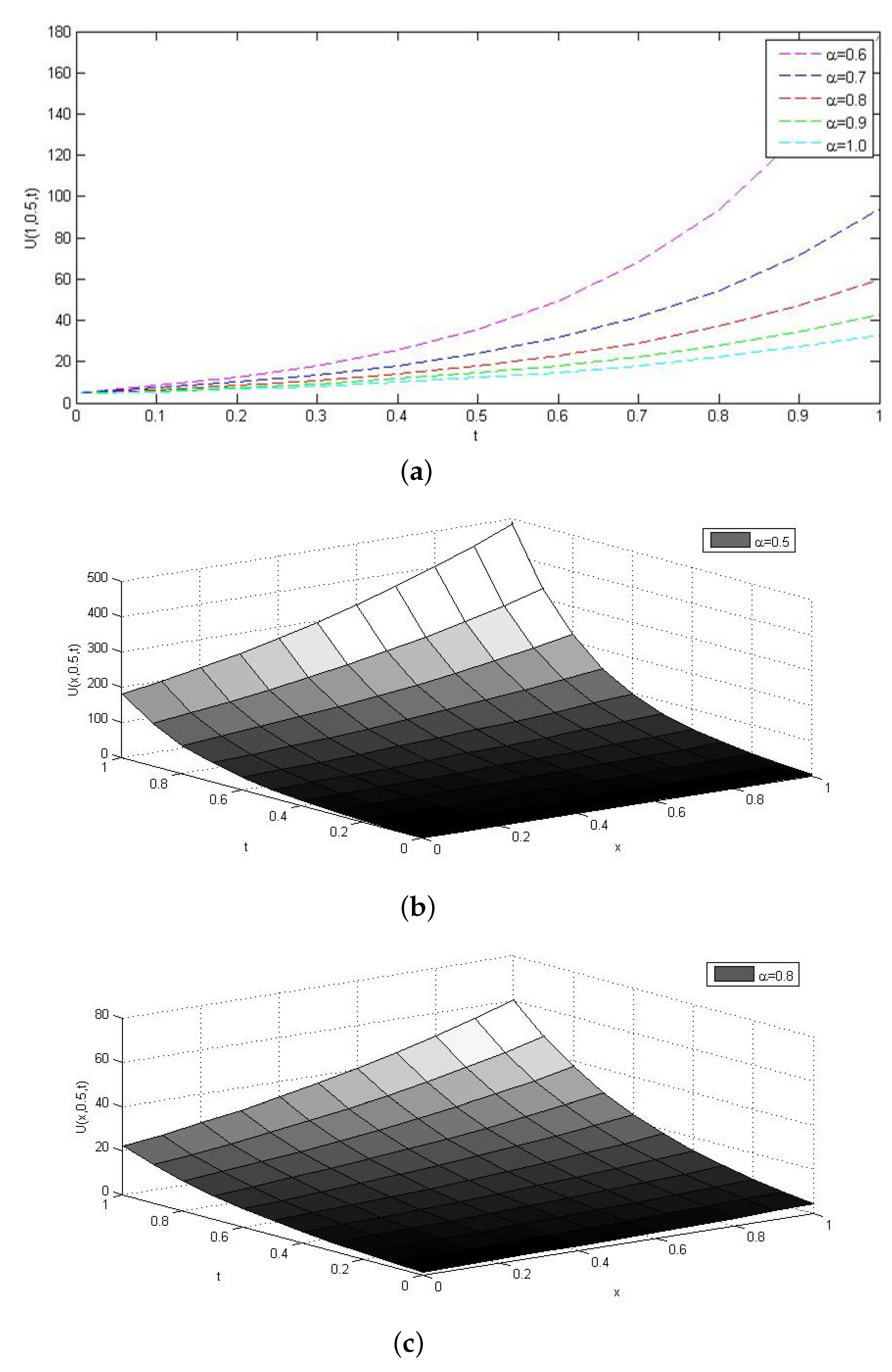
5.2. The Two-Dimensional Time Fractional Diffusion Equation

In ref. [35], Nigmatullin introduced the fractional diffusion equation in physics, which described the diffusion in media with fractal geometry. The fractional diffusion equation can also be used to describe some physical phenomena, such as Stefan problem, thermophysical process, transition flows of complex fluids and so on. In this section, we apply the HPSTM and the VILTM to the following two-dimensional time fractional diffusion equation [36]

$$\begin{array}{c}\hfill {\mathrm{D}}_t^{\alpha }U(x,y,t)={\mathrm{D}}_x^{2}U(x,y,t)+{\mathrm{D}}_y^{2}U(x,y,t),\forall x,y\in [0,1],t>0,0<\alpha ⩽1\end{array}$$

(18)

with the initial condition

$$U(x,y,0)=e^{x+y}.$$

5.2.1. Homotopy Perturbation Sumudu Transform Method

Applying the Sumudu transform to both sides of (18) and taking into account the initial condition, we obtain

$$\begin{array}{c}\hfill S[U(x,y,t)]=e^{x+y}+u^{\alpha }S[{\mathrm{D}}_x^{2}U(x,y,t)+{\mathrm{D}}_y^{2}U(x,y,t)].\end{array}$$

(19)

Then the inverse Sumudu transform of (19) implies that

$$\begin{array}{c}\hfill U(x,y,t)=e^{x+y}+S^{-1}[u^{\alpha }S[{\mathrm{D}}_x^{2}U(x,y,t)+{\mathrm{D}}_y^{2}U(x,y,t)]].\end{array}$$

(20)

Now applying the HPSTM, we obtain

$$\begin{array}{c}\hfill \sum _{n=0}^{\infty }{p}^n{U}_n(x,y,t)=e^{x+y}+p\times S^{-1}\left[u^{\alpha }S\left[{\mathrm{D}}_x^2\left(\sum _{n=0}^{\infty }{p}^n{U}_n(x,y,t)\right)+{\mathrm{D}}_y^2\left(\sum _{n=0}^{\infty }{p}^n{U}_n(x,y,t)\right)\right]\right].\end{array}$$

Comparing the coefficients with identical powers in p, we have

$$\begin{array}{cc}\hfill U_0(x,y,t)=& U(x,y,0)=e^{x+y},\hfill \\ \hfill U_1(x,y,t)=& \frac{t^{\alpha }}{\Gamma (\alpha +1)}2e^{x+y},\hfill \\ \hfill & \cdots \hfill \\ \hfill U_k(x,y,t)=& \frac{t^{k\alpha }}{\Gamma (k\alpha +1)}{2}^k{e}^{x+y},k\in \mathbb{N}.\hfill \end{array}$$

Therefore, the HPSTM series solution is

$$\begin{array}{cc}\hfill U(x,y,t)=& \sum _{k=0}^{\infty }{U}_k(x,y,t)=\sum _{k=0}^{\infty }\frac{t^{k\alpha }}{\Gamma (k\alpha +1)}{2}^k{e}^{x+y}=e^{x+y}\sum _{k=0}^{\infty }\frac{{(2t^{\alpha })}^k}{\Gamma (k\alpha +1)}.\hfill \end{array}$$

(21)

Set $\alpha =1$ in (18), we obtain the following series solution

$$\begin{array}{c}\hfill U(x,y,t)=e^{x+y}\sum _{k=0}^{\infty }\frac{{(2t)}^k}{\Gamma (k+1)}=e^{x+y+2t},\end{array}$$

(22)

which is the exact solution of (18) for $\alpha =1$. In addition, the corresponding third approximate solution is

$$\begin{array}{c}\hfill U_{app}(x,y,t)=e^{x+y}\left(1+\frac{2t}{\Gamma (2)}+\frac{4t^2}{\Gamma (3)}+\frac{8t^3}{\Gamma (4)}\right).\end{array}$$

(23)

The exact solution (22) and the third approximate solution (23) obtained by the HPSTM at $x=1,y=0.5$ for $\alpha =1$ are shown in Figure 1. It is shown from Figure 1 that the third approximate solution is nearly identical with the exact solution. The physical behaviors of the HPSTM solution (22) are shown in Figure 2. The approximate solutions of (21) for different values $\alpha \le 1$ are depicted in Figure 3. The error estimates of the approximate solutions (21) obtained by the HPSTM at $x=y=0$ for $\alpha =0.5$ are shown in Table 1, Table 2 and Table 3. It can be seen from Table 1, Table 2 and Table 3, to control the error within one thousandth, it only needs 8 steps at $t=0.1$, 20 steps at $t=0.5$ and 30 steps at $t=1$, and the time of calculation takes only a few seconds. That means this method is rapidly convergent and relatively efficient.

Figure 1. Exact solution and third approximate solution for $\alpha =1$.

Figure 2. (a) The HPSTM solution at $y=0.5$. (b) The HPSTM solution at $t=1$. (c) The HPSTM solution at $x=1$.

Figure 3. (a) Approximate solutions for different values of $\alpha \le 1$. (b) Approximate solution for $\alpha =0.5$. (c) Approximate solution for $\alpha =0.8$.

Table 1. Error estimates at $x=y=0,t=0.1$ for $\alpha =0.5$.

$\mathit{t}=0.1$	$\mathit{Exact}\mathit{Solution}$	$\mathit{Approximate}\mathit{Solution}$	$\mathit{Error}$
$n=2$	$2.4300431415$	$2.1136496465$	$0.3163934950$
$n=4$	$2.4300431415$	$2.3839562188$	$0.0460869226$
$n=6$	$2.4300431415$	$2.4250719371$	$0.0049712044$
$n=8$	$2.4300431415$	$2.4296184953$	$0.0004246462$
$n=10$	$2.4300431415$	$2.4300131524$	$0.0000299891$
$n=12$	$2.4300431415$	$2.4300413376$	$0.0000018039$
$n=14$	$2.4300431415$	$2.4300430470$	$0.0000000945$
$n=16$	$2.4300431415$	$2.4300431371$	$0.0000000044$
$n=18$	$2.4300431415$	$2.4300431413$	$0.0000000002$
$n=20$	$2.4300431415$	$2.4300431415$	$0.0000000000$
$n=22$	$2.4300431415$	$2.4300431415$	$0.0000000000$
$n=24$	$2.4300431415$	$2.4300431415$	$0.0000000000$
$n=26$	$2.4300431415$	$2.4300431415$	$0.0000000000$
$n=28$	$2.4300431415$	$2.4300431415$	$0.0000000000$
$n=30$	$2.4300431415$	$2.4300431415$	$0.0000000000$

Table 2. Error estimates at $x=y=0,t=0.5$ for $\alpha =0.5$.

$\mathit{t}=0.5$	$\mathit{Exact}\mathit{Solution}$	$\mathit{Approximate}\mathit{Solution}$	$\mathit{Error}$
$n=2$	$14.4419081954$	$4.5957691216$	$9.8461390738$
$n=4$	$14.4419081954$	$8.7234612837$	$5.7184469117$
$n=6$	$14.4419081954$	$11.7589483468$	$2.6829598486$
$n=8$	$14.4419081954$	$13.3982742876$	$1.0436339078$
$n=10$	$14.4419081954$	$14.0972339650$	$0.3446742304$
$n=12$	$14.4419081954$	$14.3433203123$	$0.0985878831$
$n=14$	$14.4419081954$	$14.4170855865$	$0.0248226089$
$n=16$	$14.4419081954$	$14.4363330458$	$0.0055777374$
$n=18$	$14.4419081954$	$14.4407788636$	$0.0011293310$
$n=20$	$14.4419081954$	$14.4416999733$	$0.0002082221$
$n=22$	$14.4419081954$	$14.4418729796$	$0.0000352158$
$n=24$	$14.4419081954$	$14.4419026959$	$0.0000054995$
$n=26$	$14.4419081954$	$14.4419073978$	$0.0000007976$
$n=28$	$14.4419081954$	$14.4419080875$	$0.0000001079$
$n=30$	$14.4419081954$	$14.4419081817$	$0.0000000144$

Table 3. Error estimates at $x=y=0,t=1$ for $\alpha =0.5$.

$\mathit{t}=1$	$\mathit{Exact}\mathit{Solution}$	$\mathit{Approximate}\mathit{Solution}$	$\mathit{Error}$
$n=2$	$108.9409043900$	$7.2567583342$	$101.6841460558$
$n=4$	$108.9409043900$	$21.2747805587$	$87.6661238313$
$n=6$	$108.9409043900$	$41.5702827846$	$67.3706216054$
$n=8$	$108.9409043900$	$63.2413329475$	$45.6995714425$
$n=10$	$108.9409043900$	$81.5563404997$	$27.3845638903$
$n=12$	$108.9409043900$	$94.3591742750$	$14.581730115$
$n=14$	$108.9409043900$	$101.9877801637$	$6.9531242263$
$n=16$	$108.9409043900$	$105.9480101826$	$2.9928942074$
$n=18$	$108.9409043900$	$107.7691538039$	$1.1717505861$
$n=20$	$108.9409043900$	$108.5207427268$	$0.4201616632$
$n=22$	$108.9409043900$	$108.8020586898$	$0.1388457002$
$n=24$	$108.9409043900$	$108.8983848776$	$0.0425195124$
$n=26$	$108.9409043900$	$108.9287781760$	$0.0121262140$
$n=28$	$108.9409043900$	$108.9376695550$	$0.0032348350$
$n=30$	$108.9409043900$	$108.9400940351$	$0.0008103549$

5.2.2. Variational Iteration Laplace Transform Method

Applying the Laplace transform to both sides of (18), the corresponding iteration formula is given by

$$\begin{array}{c}\hfill U_{n+1}(x,y,s)=U_n(x,y,s)+\lambda (s)[s^{\alpha }{U}_n(x,y,s)-e^{x+y}{s}^{\alpha -1}-L[{\mathrm{D}}_x^2{U}_n(x,y,t)+{\mathrm{D}}_y^2{U}_n(x,y,t)]].\end{array}$$

Considering $L[{\mathrm{D}}_x^2{U}_n(x,y,t)+{\mathrm{D}}_y^2{U}_n(x,y,t)]$ as restricted term, we choose the Lagrange multiplier as $\lambda =-s^{-\alpha }$. Using the inverse Laplace transform $L^{-1}$, we have the following approximate solution of (18)

$$\begin{array}{c}\hfill U_{n+1}(x,y,t)=e^{x+y}+L^{-1}\left[s^{-\alpha }L[{\mathrm{D}}_x^2{U}_n(x,y,t)+{\mathrm{D}}_y^2{U}_n(x,y,t)]\right].\end{array}$$

According to the iteration formula, we have

$$\begin{array}{cc}\hfill U_0(x,y,t)=& e^{x+y},\hfill \\ \hfill U_1(x,y,t)=& e^{x+y}+L^{-1}\left[s^{-\alpha }L[{\mathrm{D}}_x^2{U}_0(x,y,t)+{\mathrm{D}}_y^2{U}_0(x,y,t)]\right]\hfill \\ \hfill =& e^{x+y}+\frac{t^{\alpha }}{\Gamma (\alpha +1)}2e^{x+y},\hfill \\ \hfill U_2(x,y,t)=& e^{x+y}+L^{-1}\left[s^{-\alpha }L[{\mathrm{D}}_x^2{U}_1(x,y,t)+{\mathrm{D}}_y^2{U}_1(x,y,t)]\right]\hfill \\ \hfill =& e^{x+y}+\frac{t^{\alpha }}{\Gamma (\alpha +1)}2e^{x+y}+\frac{t^{2\alpha }}{\Gamma (2\alpha +1)}4e^{x+y},\hfill \\ \hfill & \cdots \hfill \\ \hfill U_k(x,y,t)=& \sum _{i=0}^k\frac{t^{i\alpha }}{\Gamma (i\alpha +1)}{2}^i{e}^{x+y}.\hfill \end{array}$$

When $k\to \infty$, the solution can be represented as

$$\begin{array}{c}\hfill U(x,y,t)=\underset{k\to \infty }{lim}{e}^{x+y}\sum _{i=0}^k\frac{{(2t^{\alpha })}^i}{\Gamma (i\alpha +1)},\end{array}$$

which is the same as the limit approximate solution by the HPSTM.

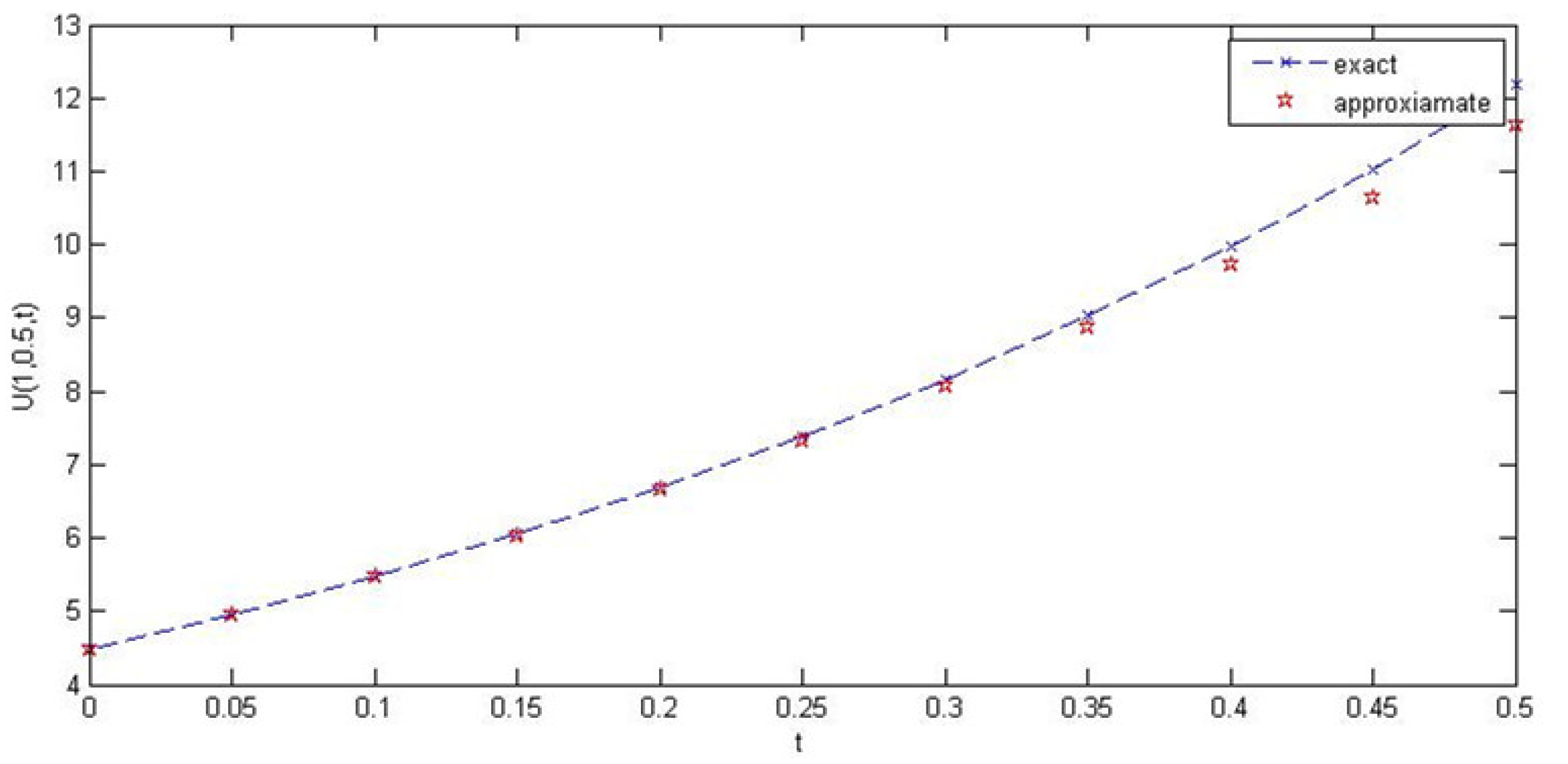
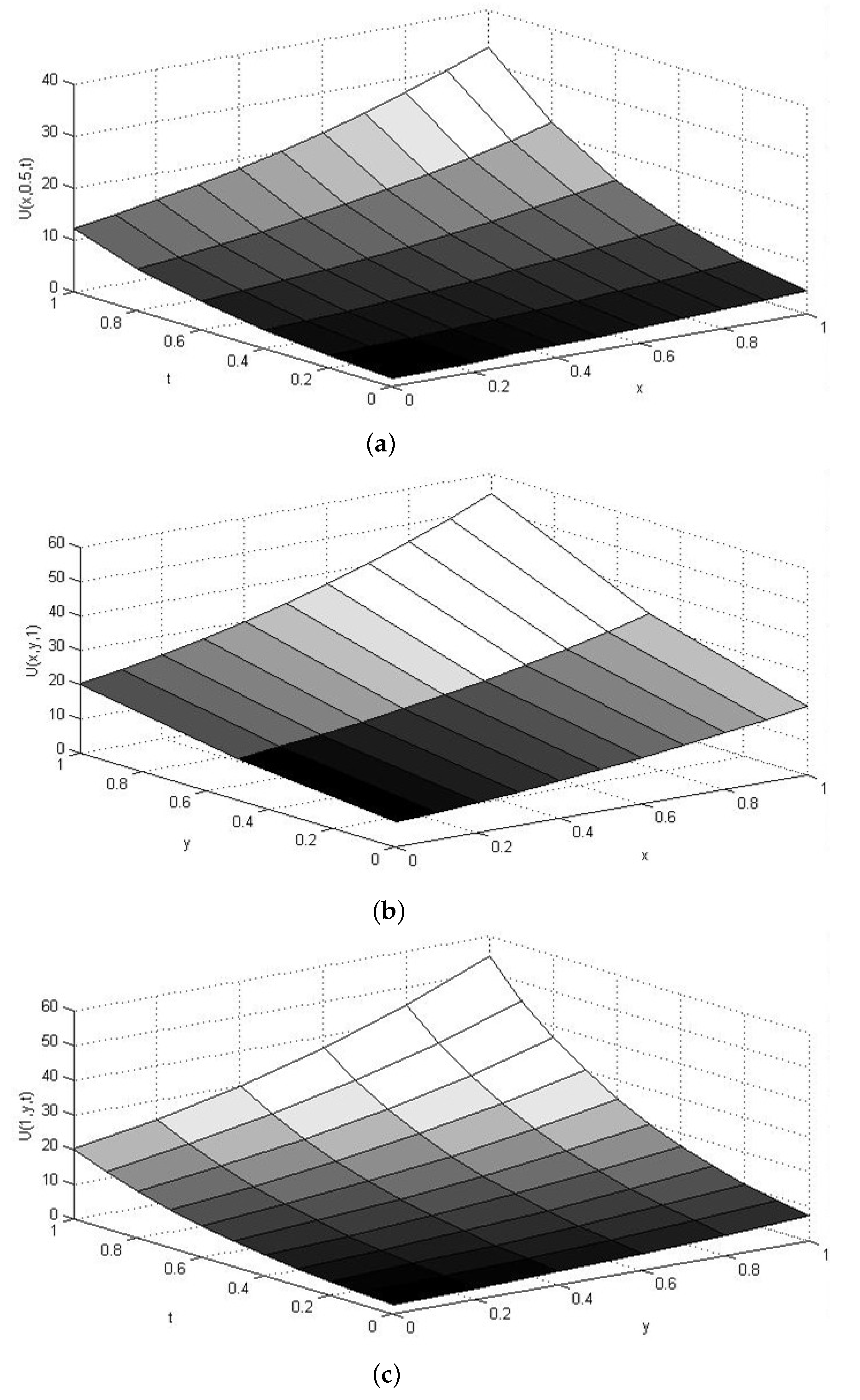
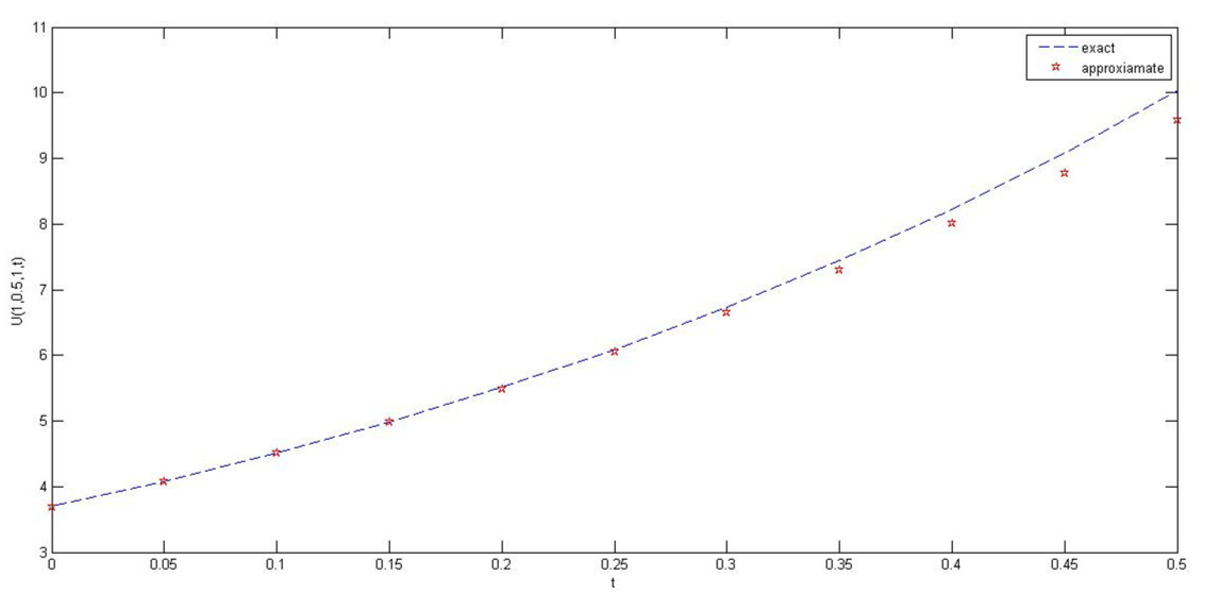
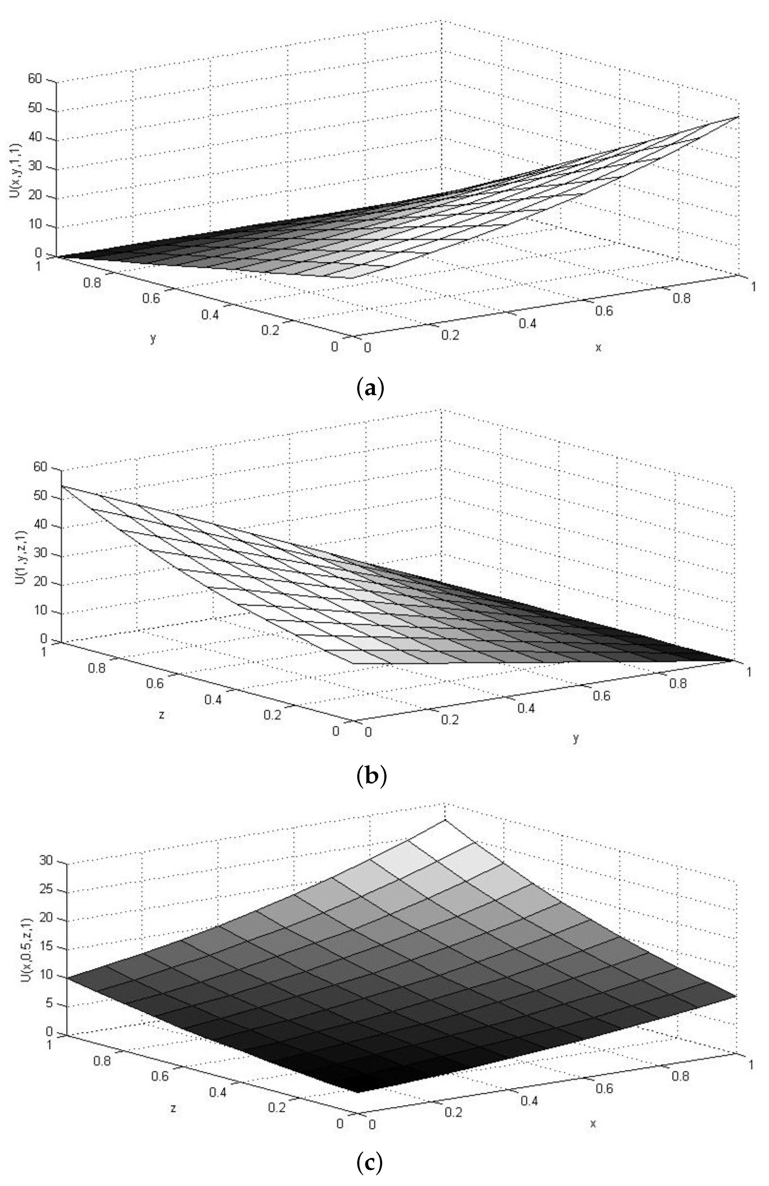
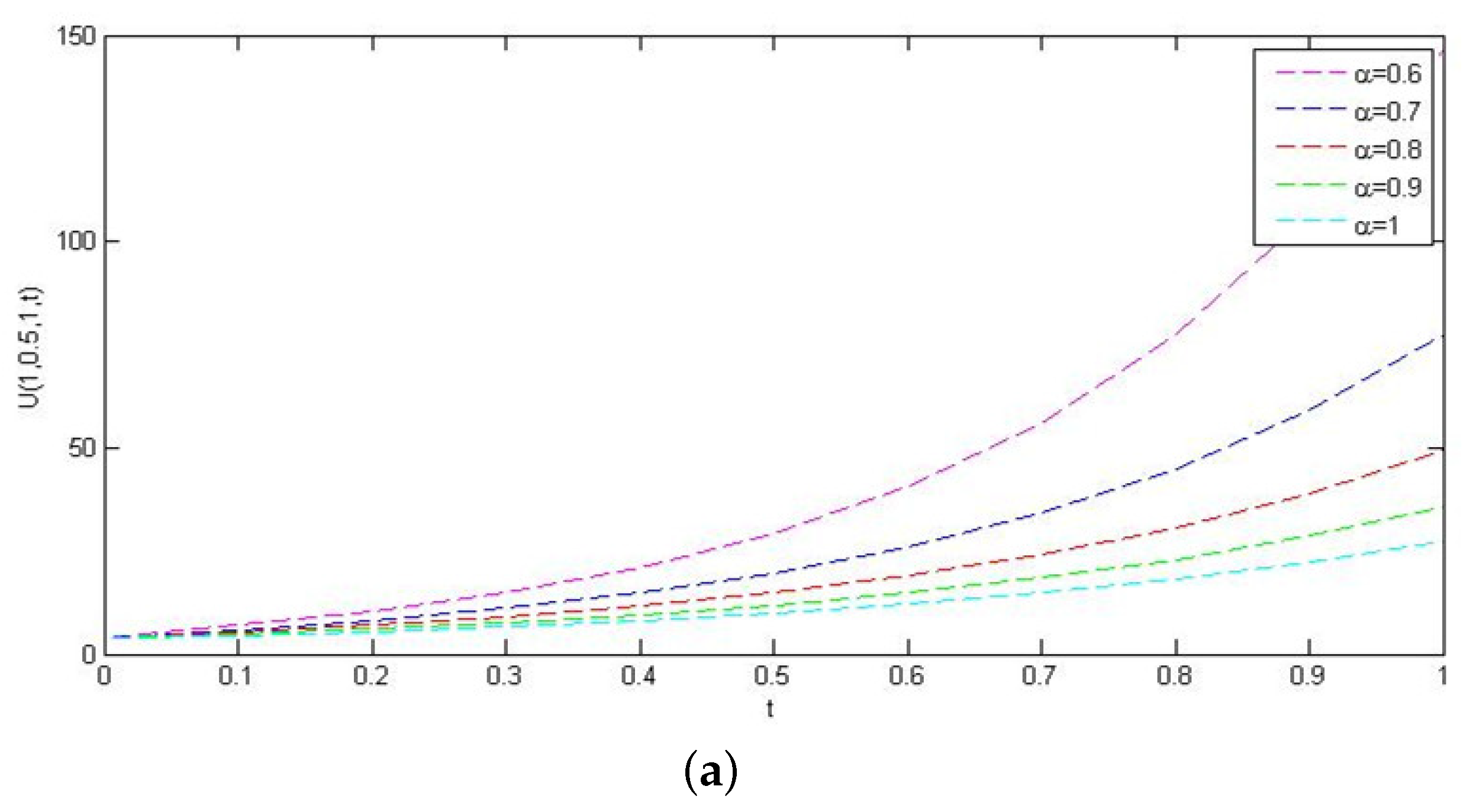
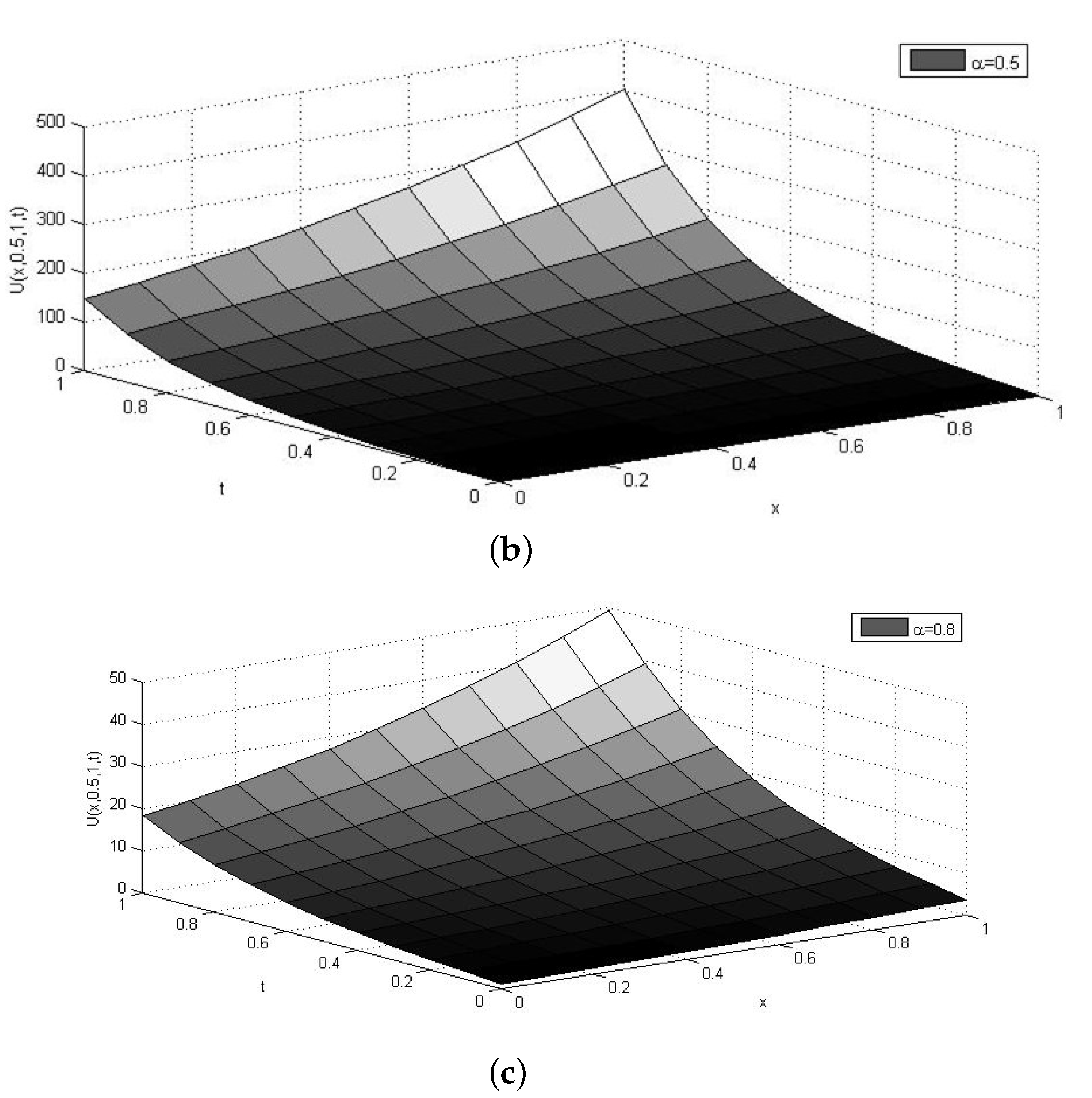
5.3. The Three-Dimensional Time Fractional Differential Equation

In this section, we apply the HPSTM and the VILTM to the following three-dimensional time fractional differential equation [36]

$$\begin{array}{c}\hfill {\mathrm{D}}_t^{\alpha }U(x,y,z,t)={\mathrm{D}}_x^{2}U(x,y,z,t)+{\mathrm{D}}_y^{2}U(x,y,z,t)+{\mathrm{D}}_z^{2}U(x,y,z,t),\forall x,y,z\in [0,1],t>0,0<\alpha ⩽1\end{array}$$

(24)

with the initial condition

$$U(x,y,z,0)=(1-y)e^{x+z}.$$

5.3.1. Homotopy Perturbation Sumudu Transform Method

Applying the Sumudu transform to both sides of (24) and taking into account the initial condition, we obtain

$$\begin{array}{c}\hfill S[U(x,y,z,t)]=(1-y)e^{x+z}+u^{\alpha }S[{\mathrm{D}}_x^{2}U(x,y,z,t)+{\mathrm{D}}_y^{2}U(x,y,z,t)+{\mathrm{D}}_z^{2}U(x,y,z,t)].\end{array}$$

(25)

The inverse Sumudu transform of (25) implies that

$$\begin{array}{c}\hfill U(x,y,z,t)=(1-y)e^{x+z}+S^{-1}[u^{\alpha }S[{\mathrm{D}}_x^{2}U(x,y,z,t)+{\mathrm{D}}_y^{2}U(x,y,z,t)+{\mathrm{D}}_z^{2}U(x,y,z,t)]].\end{array}$$

(26)

Using the HPSTM,

$$\begin{array}{cc}\hfill \sum _{n=0}^{\infty }{p}^n{U}_n(x,y,z,t)=& (1-y)e^{x+z}+p\times S^{-1}[u^{\alpha }S[{\mathrm{D}}_x^2\left(\sum _{n=0}^{\infty }{p}^n{U}_n(x,y,z,t)\right)\hfill \\ & +{\mathrm{D}}_y^2\left(\sum _{n=0}^{\infty }{p}^n{U}_n(x,y,z,t)\right)+{\mathrm{D}}_z^2\left(\sum _{n=0}^{\infty }{p}^n{U}_n(x,y,z,t)\right)]].\hfill \end{array}$$

Comparing the coefficients with identical powers in p, we have

$$\begin{array}{cc}\hfill U_0(x,y,z,t)=& (1-y)e^{x+z},\hfill \\ \hfill U_1(x,y,z,t)=& \frac{t^{\alpha }}{\Gamma (\alpha +1)}2(1-y)e^{x+z},\hfill \\ \hfill \cdots \\ \hfill U_k(x,y,z,t)=& \frac{t^{k\alpha }}{\Gamma (k\alpha +1)}{2}^k(1-y)e^{x+z},k\in \mathbb{N}.\hfill \end{array}$$

Therefore, the HPSTM series solution is

$$\begin{array}{c}\hfill U(x,y,z,t)=\sum _{k=0}^{\infty }{U}_k(x,y,z,t)=\sum _{k=0}^{\infty }\frac{t^{k\alpha }}{\Gamma (k\alpha +1)}{2}^k(1-y)e^{x+z}=(1-y)e^{x+z}\sum _{k=0}^{\infty }\frac{{(2t^{\alpha })}^k}{\Gamma (k\alpha +1)}.\end{array}$$

(27)

When $\alpha =1$, the corresponding series solution is given by

$$\begin{array}{c}\hfill U(x,y,z,t)=(1-y)e^{x+z}\sum _{k=0}^{\infty }\frac{{(2t)}^k}{\Gamma (k+1)}=(1-y)e^{x+z+2t},\end{array}$$

(28)

which is the exact solution for $\alpha =1$. In addition, the third approximate solution is

$$\begin{array}{c}\hfill U_{app}(x,y,z,t)=(1-y)e^{x+z}\left(1+\frac{2t}{\Gamma (2)}+\frac{4t^2}{\Gamma (3)}+\frac{8t^3}{\Gamma (4)}\right).\end{array}$$

(29)

The exact solution (28) and the third approximate solution (29) at $x=1,y=0.5,z=1$ for $\alpha =1$ are shown in Figure 4. It is shown from Figure 4 that the third approximate solution is closed to the exact solution. For $\alpha =1$, the approximate solutions at different values of $x,y,z,t$ are shown in Figure 5. The approximate solutions of (27) for different values $\alpha \le 1$ are depicted in Figure 6. The error estimates of the approximate solutions (27) at $x=y=z=0$ for $\alpha =0.5$ are the same as in Table 1, Table 2 and Table 3.

Figure 4. Exact solution and third approximate solution for $\alpha =1$.

Figure 5. (a) HPSTM solution at $z=1$ and $t=1$. (b) HPSTM solution at $x=1$ and $t=1$. (c) HPSTM solution at $y=0.5$ and $t=1$.

Figure 6. (a) Approximate solutions for different values of $\alpha \le 1$. (b) Approximate solution for $\alpha =0.5$. (c) Approximate solution for $\alpha =0.8$.

5.3.2. Variational Iteration Laplace Transform Method

Applying the Laplace transform to both sides of (24), we obtain the following iteration formula

$$\begin{array}{cc}\hfill U_{n+1}(x,y,z,s)=& U_n(x,y,z,s)+\lambda (s)[s^{\alpha }{U}_n(x,y,z,s)-(1-y)e^{x+z}{s}^{\alpha -1}\hfill \\ & -L[{\mathrm{D}}_x^{2}U(x,y,z,t)+{\mathrm{D}}_y^{2}U(x,y,z,t)+{\mathrm{D}}_z^{2}U(x,y,z,t)]].\hfill \end{array}$$

Considering $L[{\mathrm{D}}_x^{2}U(x,y,z,t)+{\mathrm{D}}_y^{2}U(x,y,z,t)+{\mathrm{D}}_z^{2}U(x,y,z,t)]]$ as restricted term, we can choose the Lagrange multiplier as $\lambda =-s^{-\alpha }$. Using the inverse Laplace transform $L^{-1}$, we obtain the following approximate solution of (24)

$$\begin{array}{c}\hfill U_{n+1}(x,y,z,t)=(1-y)e^{x+z}+L^{-1}\left[s^{-\alpha }L[{\mathrm{D}}_x^2{U}_n(x,y,z,t)+{\mathrm{D}}_y^2{U}_n(x,y,z,t)+{\mathrm{D}}_z^2{U}_n(x,y,z,t)]\right].\end{array}$$

According to the iteration formula, we have

$$\begin{array}{cc}\hfill U_0(x,y,z,t)=& (1-y)e^{x+z},\hfill \\ \hfill U_1(x,y,z,t)=& (1-y)e^{x+z}+L^{-1}\left[s^{-\alpha }L[{\mathrm{D}}_x^2{U}_0(x,y,z,t)+{\mathrm{D}}_y^2{U}_0(x,y,z,t)++{\mathrm{D}}_z^2{U}_0(x,y,z,t)]\right]\hfill \\ \hfill =& (1-y)e^{x+z}+\frac{t^{\alpha }}{\Gamma (\alpha +1)}2(1-y)e^{x+z},\hfill \\ \hfill U_2(x,y,z,t)=& (1-y)e^{x+z}+L^{-1}\left[s^{-\alpha }L[{\mathrm{D}}_x^2{U}_1(x,y,z,t)+{\mathrm{D}}_y^2{U}_1(x,y,z,t)++{\mathrm{D}}_z^2{U}_1(x,y,z,t)]\right]\hfill \\ \hfill =& (1-y)e^{x+z}+\frac{t^{\alpha }}{\Gamma (\alpha +1)}2(1-y)e^{x+z}+\frac{t^{2\alpha }}{\Gamma (2\alpha +1)}4(1-y)e^{x+z},\hfill \\ \hfill & \cdots \hfill \\ \hfill U_k(x,y,z,t)=& \sum _{i=0}^k\frac{t^{i\alpha }}{\Gamma (i\alpha +1)}{2}^i(1-y)e^{x+z}.\hfill \end{array}$$

When $k\to \infty$, we obtain the following series solution

$$\begin{array}{c}\hfill U(x,y,z,t)=\underset{k\to \infty }{lim}(1-y)e^{x+z}\sum _{i=0}^k\frac{{(2t^{\alpha })}^i}{\Gamma (i\alpha +1)},\end{array}$$

which is the same as the limit approximate solution by the HPSTM.

6. Conclusions

In this paper, we investigate the time–space fractional differential equations by the HPSTM and the VILTM. It can be concluded that these two methods are both important and efficient for obtaining approximate analytical solutions of fractional differential equations. The approximate solutions obtained by the HPSTM are uniformly valid not only for small parameters, but also for very large parameter $p\in [0,1]$, which is considered to be a “expansion parameter”. The VILTM does not require specific transformations for nonlinear term as required by some existing techniques.

Comparing these two methods with other classical methods, we know that the approximate solutions can be constructed without using any overstrict assumption or linearization, and the solutions are represented as convergent series with easily computable components and rapid convergence. The advantages of these two methods are their flexibility and ability to solve nonlinear equations efficiently and conveniently, and they not only reduce the volume of computational work but also maintain a high accuracy of the solutions. Meanwhile, the high agreement of solutions obtained by the HPSTM and the VILTM reinforces the conclusion that the efficiency of these two methods.

References

- Ross, B. The development of fractional calculus 1695–1900. Historia Math. 1977, 4, 75–89. [Google Scholar] [CrossRef] [Green Version]
- Bhatter, S.; Mathur, A.; Kumar, D.; Singh, J. A new analysis of fractional Drinfeld-Sokolov-Wilson model with exponential memory. Physica A 2020, 537, 122578. [Google Scholar] [CrossRef]
- Goswami, A.; Singh, J.; Kumar, D. An efficient analytical approach for fractional equal width equations describing hydro-magnetic waves in cold plasma. Physica A 2019, 524, 563–575. [Google Scholar] [CrossRef]
- Jena, R.M.; Chakraverty, S.; Jena, S.K. Analysis of the dynamics of phytoplankton nutrient and whooping cough models with nonsingular kernel arising in the biological system. Chaos Solitons Fractals 2020, 141, 1–10. [Google Scholar] [CrossRef]
- Kumar, D.; Singh, J.; Tanwar, K.; Baleanu, D. A new fractional exothermic reactions model having constant heat source in porous media with power, exponential and Mittag-Leffler laws. Int. J. Heat Mass Transf. 2019, 138, 1222–1227. [Google Scholar] [CrossRef]
- Singh, J.; Kumar, D.; Hammouch, Z.; Atangana, A. A fractional epidemiological model for computer viruses pertaining to a new fractional derivative. Appl. Math. Comput. 2018, 316, 504–515. [Google Scholar] [CrossRef]
- Veeresha, P.; Prakasha, D.G.; Kumar, D. Fractional SIR epidemic model of childhood disease with Mittag-Leffler memory. In Fractional Calculus in Medical and Health Science; CRC Press: Boca Raton, FL, USA, 2020; pp. 229–248. [Google Scholar]
- Zhang, Z.Z. A novel COVID-19 mathematical model with fractional derivatives: Singular and nonsingular kernels. Chaos Solitons Fractals 2020, 139, 1–11. [Google Scholar] [CrossRef]
- Miller, K.S.; Ross, B. An Introduction to the Fractional Calculus and Fractional Differential Equations; John Wiley & Sons, Inc.: New York, NY, USA, 1993. [Google Scholar]
- Adomian, G. Solving Frontier Problems of Physics: The Decomposition Method; Kluwer Academic: Boston, MA, USA, 1994. [Google Scholar]
- Farman, M.; Saleem, M.; Ahmad, A.; Ahmad, M. Analysis and numerical solution of SEIR epidemic model of measles with non-integer time fractional derivatives by using laplace adomian decomposition method. Ain. Shams. Eng. J. 2018, 9, 3391–3397. [Google Scholar] [CrossRef]
- Fadugba, S.E. Homotopy analysis method and its applications in the valuation of European call options with time-fractional Black-Scholes equation. Chaos Solitons Fractals 2020, 141, 110351. [Google Scholar] [CrossRef]
- Liao, S.J. Homotopy analysis method: A new analytic method for nonlinear problems. Commun. Nonlinear Sci. Numer. Simul. 1998, 3, 159–163. [Google Scholar] [CrossRef]
- Van Gorder, R.A. The variational iteration method is a special case of the homotopy analysis method. Appl. Math. Lett. 2015, 45, 81–85. [Google Scholar] [CrossRef]
- He, J.H. Approximate analytical solution for seepage flow with fractional derivatives in porous media. Comput. Methods Appl. Mech. Engrg. 1998, 167, 57–68. [Google Scholar] [CrossRef]
- Sakar, M.G.; Ergören, H. Alternative variational iteration method for solving the time-fractional Fornberg-Whitham equation. Appl. Math. Model. 2015, 39, 3972–3979. [Google Scholar] [CrossRef]
- He, J.H. Homotopy perturbation technique. Comput. Methods Appl. Mech. Eng. 1999, 178, 257–262. [Google Scholar] [CrossRef]
- Jleli, M.; Kumar, S.; Kumar, R.; Samet, B. Analytical approach for time fractional wave equations in the sense of Yang-Abdel-Aty-Cattani via the homotopy perturbation transform method. Alex. Eng. J. 2020, 59, 2859–2863. [Google Scholar] [CrossRef]
- He, J.H. Exp-function method for nonlinear wave equations. Chaos Solitons Fractals 2006, 30, 700–708. [Google Scholar] [CrossRef]
- Zulfiqar, A.; Ahmad, J. Soliton solutions of fractional modified unstable Schrödinger equation using Exp-function method. Results Phys. 2020, 19, 103476. [Google Scholar] [CrossRef]
- Lu, D.C.; Suleman, M.; He, J.H.; Farooq, U.; Noeiaghdam, S.; Chandio, F.A. Elzaki projected differential transform method for fractional order system of linear and nonlinear fractional partial differential equation. Fractals 2018, 3, 1850041. [Google Scholar] [CrossRef]
- Singh, J.; Kumar, D.; Sushila, D. Homotopy perturbation Sumudu transform method for nonlinear equations. Adv. Theor. Appl. Mech. 2011, 4, 165–175. [Google Scholar]
- Sharma, D.; Singh, P.; Chauhan, S. Homotopy perturbation Sumudu transform method with He’s polynomial for solutions of some fractional nonlinear partial differential equations. Int. J. Nonlinear Sci. 2016, 21, 91–97. [Google Scholar]
- Wu, G.C.; Baleanu, D. Variational iteration method for fractional calculus-a universal approach by laplace transform. Adv. Differ. Equ. 2013, 2013, 18. [Google Scholar] [CrossRef] [Green Version]
- Liu, Y.; Yin, X.; Zhao, L. Approximate solutions of fractional wave equations using variational iteration method and Laplace transform. Electron. J. Math. Anal. Appl. 2015, 3, 297–303. [Google Scholar]
- Wu, G.C. Laplace transform overcoming principle drawbacks in application of the variational iteration method to fractional heat equations. Therm. Sci. 2012, 16, 1257–1261. [Google Scholar] [CrossRef]
- Yulita Molliq, R.; Noorani, M.S.M.; Hashim, I. Variational iteration method for fractional heat- and wave-like equations. Nonlinear Anal. Real World Appl. 2009, 10, 1854–1869. [Google Scholar] [CrossRef]
- Watugala, G.K. Sumudu transform: A new integral transform to solve differential equations and control engineering problems. Int. J. Math. Ed. Sci. Tech. 1993, 24, 35–43. [Google Scholar] [CrossRef]
- Aşiru, M.A. Further properties of the Sumudu transform and its applications. Int. J. Math. Ed. Sci. Tech. 2002, 33, 441–449. [Google Scholar] [CrossRef]
- Katatbeh, Q.D.; Belgacem, F.B.M. Applications of the Sumudu transform to fractional differential equations. Nonlinear Stud. 2011, 18, 99–112. [Google Scholar]
- Elbeleze, A.A.; Kılıçman, A.; Taib, B.M. Note on the convergence analysis of homotopy perturbation method for fractional partial differential equations. Abstr. Appl. Anal. 2014, 2014, 803902. [Google Scholar] [CrossRef]
- Abbaoui, K.; Cherruault, Y. New ideas for proving convergence of decomposition methods. Comput. Math. Appl. 1995, 29, 103–108. [Google Scholar] [CrossRef] [Green Version]
- Elbeleze, A.A.; Kılıçman, A.; Taib, B.M. Convergence of variational iteration method for solving singular partial differential equations of fractional order. Abstr. Appl. Anal. 2014, 2014, 518343. [Google Scholar] [CrossRef]
- Momani, S. An explicit and numerical solutions of the fractional KdV equation. Math. Comput. Simul. 2005, 70, 110–118. [Google Scholar] [CrossRef]
- Nigmatullin, R.R. The realization of the generalized transfer equation in a medium with fractal geometry. Phys. Status Solidi (b) 1986, 133, 425–430. [Google Scholar] [CrossRef]
- Kumar, D.; Singh, J.; Kumar, S. Numerical computation of fractional multi-dimensional diffusion equations by using a modified homotopy perturbation method. J. Assoc. Arab. Univ. Basic Appl. Sci. 2015, 17, 20–26. [Google Scholar] [CrossRef] [Green Version]
Publisher’s Note: MDPI stays neutral with regard to jurisdictional claims in published maps and institutional affiliations. |
© 2021 by the authors. Licensee MDPI, Basel, Switzerland. This article is an open access article distributed under the terms and conditions of the Creative Commons Attribution (CC BY) license (https://creativecommons.org/licenses/by/4.0/).