Abstract
The nature of the kernel density estimator (KDE) is to find the underlying probability density function (p.d.f) for a given dataset. The key to training the KDE is to determine the optimal bandwidth or Parzen window. All the data points share a fixed bandwidth (scalar for univariate KDE and vector for multivariate KDE) in the fixed KDE (FKDE). In this paper, we propose an improved variable KDE (IVKDE) which determines the optimal bandwidth for each data point in the given dataset based on the integrated squared error (ISE) criterion with the regularization term. An effective optimization algorithm is developed to solve the improved objective function. We compare the estimation performance of IVKDE with FKDE and VKDE based on ISE criterion without regularization on four univariate and four multivariate probability distributions. The experimental results show that IVKDE obtains lower estimation errors and thus demonstrate the effectiveness of IVKDE.
1. Introduction
It is very important for many machine learning algorithms to estimate the unknown probability density functions (p.d.f.s) of given datasets, e.g., Bayesian classifiers [1,2], density-based clustering algorithms [3,4], and mutual information-based feature selection algorithms [5,6]. In order to obtain the unknown p.d.f., an effective kernel density estimator (KDE) should be thoroughly constructed in advance. The classical KDE training method is the Parzen window method [7], which uses the superposition of multiple kernel functions with a fixed Parzen window (i.e., bandwidth) to fit the unknown p.d.f. The most used kernels [8] include uniform, triangular, Epanechnikov, biwieght, triweight, cosine, and Gaussian kernels. Compared with the kernels, the bandwidth plays a more important role in p.d.f. estimation: a large bandwidth will result in an over-smoothed estimation, while a small bandwidth will lead to an under-smoothed estimation.
How to determine an optimal bandwidth is a key point for training a KDE. In order to select an appropriate bandwidth, the effective error criterion should firstly be designed [9]. Commonly used error criteria include the integrated squared error (ISE) and the mean integrated squared error (MISE). Currently, there are two main ways to design KDE, i.e, the classical Parzen window method with the fixed bandwidth parameter named the fixed kernel density estimator (FKDE) and the modified Parzen window method with the variable bandwidth parameter named the variable kernel density estimator (VKDE). The representative studies corresponding to FKDE and VKDE are summarized as follows.
- Fixed kernel density estimator. The rule-of-thumb-based KDE (RoT-KDE) [10] was designed based on the asymptotic MISE (AMISE) criterion by assuming the unknown p.d.f. as normal p.d.f. Due to the inappropriate assumption of the true p.d.f., RoT-KDE is a naive KDE and inclined to select the over-smoothed bandwidth [8]. Apart from the sample and direct RoT-KDE, there are three other sophisticated KDEs, i.e., bootstrap-based KDE (BS-KDE) [11], biased cross-validation-based KDE (BCV-KDE) [12], and unbiased cross-validation-based KDE (UCV-KDE) [13]. BS-KDE determined the optimal bandwidth based on the MISE criterion by using the bootstrap technology to estimate the true p.d.f. BCV-KDE was also designed based on the MISE criterion, which calulated the optimal bandwidth by establishing the relationship between the true p.d.f. and the derivative of the estimated p.d.f. UCV-KDE used the ISE criterion to optimize the bandwidth by representing the true p.d.f. with the estimated leave-one-out p.d.f. In RoT-KDE, BS-KDE, BCV-KDE, and UCV-KDE, all samples in the given dataset enjoy a fixed bandwidth and do not use the bandwidth to adjust the roles of data points for p.d.f. estimation.
- Variable kernel density estimator. The model of VKDE was firstly proposed by Breiman et al. [14], who introduced the variable bandwidths for each data point in the given dataset and represented the bandwidth with distance from the data point to its k-th nearest neighbor. Jones [15] clarified the difference between VKDE employing a different bandwidth for each data point and VKDE with bandwidth as a function of estimation location. Terrell and Scott [16] derived the optimization rule for variable bandwidths based on the asymptotic mean squared error (AMSE) criterion. Hall et al. [17] improved the VKDE proposed in [16] by further analyzing the rates of VKDE convergence. Wu et al. [18] proposed a strategy to express the variable bandwidth in VKDE as the product of a local bandwidth factor and a global smoothing parameter. Suaray [19] proposed a VKDE for the p.d.f. estimation of censored data. Klebanov [20] proposed an axiomatic approach to construct a VKDE which guaranteed the density estimation invariance under linear transformations of original density as well as under splitting of density into several well-separated parts.
Compared with FKDEs, the main merit of VKDEs is that the variable bandwidths can flexibly adjust the importance of data points during the p.d.f estimation. This paper focuses on the improvement of VKDE. Jones [21] discussed the roles of ISE and MISE criteria in p.d.f. estimation. We consider using the ISE criterion to calculate the optimal bandwidths for the VKDE. The mathematical analysis indicates that the ISE criterion usually leads to an over-smoothed p.d.f. estimation. Inspired by the integration of empirical and structural risks, we propose an improved variable KDE (IVKDE) which determines the optimal bandwidth for each data point based on the ISE criterion with an regularization term in this paper. The ISE and regularization represent the empirical and structural risks for constructing VKDE, respectively. In order to obtain the optimally variable bandwidths, an effective optimization scheme is developed to solve the improved objective function. We conduct the exhaustive experiments to validate the rationality, feasibility, and effectiveness of IVKDE. The experimental results show that IVKDE is convergent and able to obtain the desirable p.d.f. estimation. In comparison with FKDE and VKDE based on the ISE criterion without regularization on four univariate and four multivariate probability distributions, IVKDE obtains lower estimation errors and thus demonstrate the effectiveness of IVKDE.
The remainder of this paper is organized as follows. In Section 2, we describe the basic principles of the variable kernel density estimator. In Section 3, we introduce the improved variable kernel density estimator. In Section 4, we provide experimental results and analysis. Finally, in Section 5, we conclude this paper and discuss future works.
2. Basic Principle of VKDE
For the given dataset , the classical fixed KDE (FKDE), i.e., Parzen window method [7], is constructed as
where
is the -variate Gaussian kernel, and , is the bandwidth. Substituting Equation (2) into Equation (1) yields the estimated p.d.f. of dataset as
where
is the -dimensional Gaussian distribution with mean vector and covariance matrix . Equation (3) reflects that the estimated p.d.f. is the superposition of Gaussian p.d.f.s.
The p.d.f. of dataset estimated by VKDE is
where the covariance matrix of is , , . Equation (5) can be further transformed into the following Equation (6):
where is the variable bandwidth vector corresponding to the n-th data point. There are bandwidth parameters which need to be determined in VKDE.
3. Proposed IVKDE
In this section, we firstly provide an improved VKDE which uses an regularization term-based objective function to evaluate the efficiency of variable bandwidths. Then, a bandwidth optimization algorithm is developed to solve the optimal variable bandwidths based on the above-mentioned objective function.
The purpose of VKDE training is to make the estimated p.d.f. as close to the true p.d.f. as possible. In Equation (6), we can find that the performance of VKDE is only related to the selection of bandwidth vectors. We want to select the bandwidth vectors which can minimize the error between p.d.f. and . In order to measure the estimated error, an effective error criterion should firstly be designed. The integrated squared error (ISE)
is used in our proposed IVKDE to measure the estimated error.
In Equation (7), we can see that the third term is unrelated to the unknown bandwidth vectors. Thus, the optimal variable bandwidth vectors can be obtained by minimizing the simplified ISE criterion:
Equation (8) is a data-driven error measurement which easily leads to a data-adaptive KDE and further makes the estimated p.d.f. more inclined to fit the given dataset . In order to guarantee the good generalization capability of KDE, we give the following objective function to select the bandwidth vectors for our proposed IVKDE:
where the second term is the regulation term, is the norm of bandwidth vector , , and is the regulation factor.
Substituting Equation (6) into and terms yields
and
respectively, where , is a leave-one-out estimator trained through an unbiased cross-validation (UCV) method.
IVKDE needs to use the optimal bandwidth vectors that can minimize the objective function with the regulation term. In order to solve the optimal bandwidths, we should firstly calculate the partial derivative of with respect to . Let
where
and
We can find that it is very difficult to calculate the analytic solution of from . Here, we design the following Algorithm 1 which uses the gradient descent method to solve the optimal bandwidths for IVKDE based on the objective function as shown in Equation (9). Algorithm 1 iteratively determines the optimal bandwidths based on the decaying learning rate adjustment. Because the minimization of is required, the negative gradient is used in Algorithm 1.
| Algorithm 1 Solving the optimal bandwidths for IVKDE. |
|
4. Experimental Results and Analysis
We conduct three experiments based on eight different probability distributions as shown in Table 1 to validate the rationality, feasibility, and effectiveness of the proposed IVKDE. The graphics of these eight p.d.f.s for the given parameters are presented in Figure 1.

Table 1.
Four univariate and four multivariate probability distributions ( in bimodal, trimodal, and quadrimodal normal distributions is the two-dimensional normal distribution with mean vector and covariance matrix ).
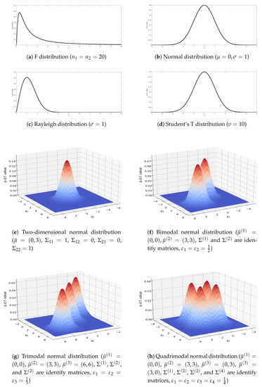
Figure 1.
Graphics of eight p.d.f.s.
4.1. Experiential Setup
The rationality is to check the convergence of Algorithm 1, the feasibility is to show the estimation capability of IVKDE to the given p.d.f.s, and the effectiveness is demonstrated by comparing the estimation performances of IVKDE with FKDE and VKDE. For FKDE and VKDE, the optimal bandwidths are also determined with the gradient descent method. The synthetic datasets obeying the above-mentioned distributions can be accessible in any country accessed via our BaiduPan (https://pan.baidu.com/s/1YhkkrckQA_e2GNd8haLE1g, accessed on 25 June 2021) with extraction code vn6j. All the estimators are implemented with the Python programming language and run on a PC with an Intel(R) Quad-core 3.00 GHz i5-7400 CPU and 16 GB memory.
4.2. Rationality of IVKDE
We test the convergence of Algorithm 1 based on the random data points obeying F, normal, two-dimensional normal, and bimodal normal distributions with the following parameters:
- F: and ;
- Normal: , , and ;
- Two-dimensional normal: , , and ;
- Bimodal normal: , , , , and .
For each distribution, we repeat the running of Algorithm 1 10 times with the following parameters: , , , , and . We check the variation of the bandwidth sum with an increase in iteration numbers, where the bandwidth sum is calculated as
In Figure 2, we can see that Algorithm 1 is convergent for the different regulation factor s on the given p.d.f. The curves of bandwidth sums firstly decrease and then keep stable with the increase in iteration numbers. This indicates that Algorithm 1 is convergent and can find the optimal bandwidths for IVKDE.
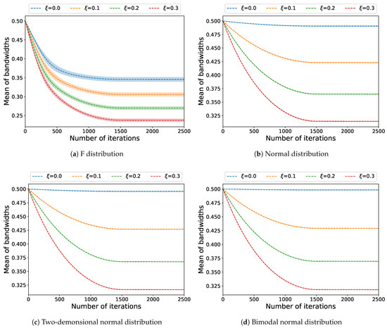
Figure 2.
Convergences of Algorithm 1 on 4 given p.d.f.s.
4.3. Feasibility of IVKDE
We check the p.d.f. estimation capability of IVKDE based on F and two-dimensional normal distributions with the following parameters:
- F: and ;
- Two-dimensional normal: , , and .
We use Algorithm 1 to determine the optimal bandwidths for each distribution based on the random data points, where the parameters of Algorithm 1 are set as , , , , , for F distribution and , , , , , and for two-dimensional normal distribution. The estimated p.d.f.s are presented in Figure 3 and Figure 4. In these two figures, we can intuitively find that IVKDE can estimate the underlying p.d.f.s based on the given data points. The estimated p.d.f.s are very close to the true p.d.f.s. The experimental results show that IVKDE is feasible to estimate the unknown p.d.f.
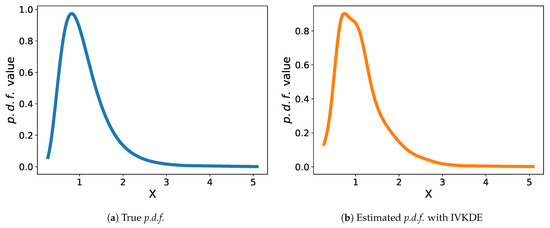
Figure 3.
Estimation capability of IVKDE on F distribution.
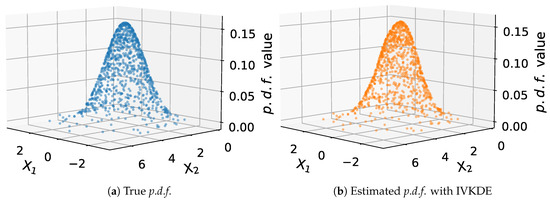
Figure 4.
Estimation capability of IVKDE on two-dimensional normal distribution.
4.4. Effectiveness of IVKDE
On eight probability distributions, as shown in Table 1, we compare the p.d.f. estimation performance of IVKDE with FKDE and VKDE. The parameters of these three kernel density estimators are summarized in Table 2. The comparative results among FKDE, VKDE, and IVKDE are listed in Table 3. We use the mean absolute error (MAE) to evaluate the training and testing performances of these three kernel density estimators. Assume the true and estimated p.d.f. values for the given dataset are and , respectively. Then, the MAE on dataset is calculated as
Table 2.
Parameter settings of FKDE, VKDE, and IVKDE.
Table 3.
Competitive results among FKDE, VKDE, and IVKDE on 8 different probability distributions.
In Table 3, we can find that IVKDE obtains the significantly better p.d.f. estimation performances on training and testing datasets than FKDE and VKDE. We carry out the statistical test on the comparative results based on the sign test method [22]. For the pairwise comparison between methods A and B, A is significantly better than B under the given significance level if the number of A’s wins reaches the critical number. There are eight different probability distributions which are used to compare the estimation performances of FKDE, VKDE, and IVKDE. The critical win number is in our comparison for the given significance level 0.05. The win numbers of IVKDE vs. FKDE and VKDE on training datasets are 7 and 8, respectively. This indicates that IVKDE obtains significantly better p.d.f. estimation performances than FKDE and VKDE on training datasets. The win numbers of IVKDE vs. FKDE and VKDE on testing datasets are 6 and 8, respectively. This indicates that IVKDE obtains significantly better p.d.f. estimation performances than VKDE on testing datasets. The experimental and statistical results show that IVKDE can improve the p.d.f. estimation performance of VKDE and thus demonstrate the effectiveness of IVKDE.
5. Conclusions and Future Works
This paper presented an improved variable kernel density estimator (IVKDE) by using both integrated squared error (ISE) and regularization to determine the optimal bandwidths. The regularization can effectively avoid the over-smoothed bandwidth selection. The experimental results demonstrated the rationality, feasibility, and effectiveness of the proposed IVKDE. Future works will be carried out according to the following research directions: (1) using IVKDE to estimate the unknown p.d.f. for a large-scale dataset [23] and (2) finding the practical applications for IVKDE in data mining and machine learning fields.
Author Contributions
Methodology, Y.J.; Writing—Original Draft Preparation, Writing—Review and Editing, Y.H.; Validation, D.H. All authors have read and agreed to the published version of the manuscript.
Funding
This paper was supported by the Basic Research Foundation of Strengthening Police with Science and Technology of the Ministry of Public Security (2017GABJC09), Open Foundation of Key Laboratory of Impression Evidence Examination and Identification Technology, The Ministry of Public Security of the People’s Republic of China (HJKF201901), Basic Research Foundation of Shenzhen (20210312191246002), and the Scientific Research Foundation of Shenzhen University for Newly-Introduced Teachers (2018060).
Data Availability Statement
The data presented in this study are available in BaiduPan https://pan.baidu.com/s/1YhkkrckQA_e2GNd8haLE1g (accessed on 25 June 2021) with extraction code vn6j.
Acknowledgments
We would like to thank the editors and two anonymous reviewers whose meticulous readings and valuable suggestions helped us to improve this paper significantly after two rounds of review.
Conflicts of Interest
The authors declare no conflict of interest.
Abbreviations
| p.d.f. | Probability Density Function |
| KDE | Kernel Density Estimator |
| ISE | Integrated Squared Error |
| MISE | Mean Integrated Squared Error |
| FKDE | Fixed Kernel Density Estimator |
| VKDE | Variable Kernel Density Estimator |
| RoT | Rule-of-Thumb |
| BS | Bootstrap |
| BCV | Biased Cross-Validation |
| UCV | Unbiased Cross-Validation |
| IVKDE | Improved Variable Kernel Density Estimator |
| MAE | Mean Absolute Error |
References
- John, G.H.; Langley, P. Estimating continuous distributions in Bayesian classifiers. In Proceedings of the Eleventh Conference on Uncertainty in Artificial Intelligence, San Francisco, CA, USA, 18–20 August 1995; pp. 338–345. [Google Scholar]
- Wang, X.Z.; He, Y.L.; Wang, D.D. Non-naive Bayesian classifiers for classification problems with continuous attributes. IEEE Trans. Cybern. 2014, 44, 21–39. [Google Scholar] [CrossRef] [PubMed]
- Azzalini, A.; Menardi, G. Clustering via nonparametric density estimation: The R package pdfCluster. J. Stat. Softw. 2014, 57, 1–26. [Google Scholar] [CrossRef] [Green Version]
- Cuevas, A.; Febrero, M.; Fraiman, R. Cluster analysis: A further approach based on density estimation. Comput. Stat. Data Anal. 2001, 36, 441–459. [Google Scholar] [CrossRef]
- Kwak, N.; Choi, C.H. Input feature selection by mutual information based on Parzen window. IEEE Trans. Pattern Anal. Mach. Intell. 2002, 24, 1667–1671. [Google Scholar] [CrossRef] [Green Version]
- Peng, H.C.; Long, F.H.; Ding, C. Feature selection based on mutual information criteria of max-dependency, max-relevance, and min-redundancy. IEEE Trans. Pattern Anal. Mach. Intell. 2005, 27, 1226–1238. [Google Scholar] [CrossRef] [PubMed]
- Parzen, E. On estimation of a probability density function and mode. Ann. Math. Stat. 1962, 33, 1065–1076. [Google Scholar] [CrossRef]
- Wand, M.P.; Jones, M.C. Kernel Smoothing; Chapman and Hall: London, UK, 1994. [Google Scholar]
- Silverman, B.W. Density Estimation for Statistics and Data Analysis; Routledge: Abingdon, UK, 2018. [Google Scholar]
- Chen, S. Optimal bandwidth selection for kernel density functionals estimation. J. Probab. Stat. 2015, 2015, 242683. [Google Scholar] [CrossRef] [Green Version]
- Taylor, C.C. Bootstrap choice of the smoothing parameter in kernel density estimation. Biometrika 1989, 76, 705–712. [Google Scholar] [CrossRef]
- Scott, D.W.; Terrell, G.R. Biased and unbiased cross-validation in density estimation. J. Am. Stat. Assoc. 1987, 82, 1131–1146. [Google Scholar] [CrossRef]
- Bowman, A.W. An alternative method of cross-validation for the smoothing of density estimates. Biometrika 1984, 71, 353–360. [Google Scholar] [CrossRef]
- Breiman, L.; Meisel, W.; Purcell, E. Variable kernel estimates of multivariate densities. Technometrics 1977, 19, 135–144. [Google Scholar] [CrossRef]
- Jones, M.C. Variable kernel density estimates and variable kernel density estimates. Aust. J. Stat. 1990, 32, 361–371. [Google Scholar] [CrossRef]
- Terrell, G.R.; Scott, D.W. Variable kernel density estimation. Ann. Stat. 1992, 20, 1236–1265. [Google Scholar] [CrossRef]
- Hall, P.; Hu, T.C.; Marron, J.S. Improved variable window kernel estimates of probability densities. Ann. Stat. 1995, 23, 1–10. [Google Scholar] [CrossRef]
- Wu, T.J.; Chen, C.F.; Chen, H.Y. A variable bandwidth selector in multivariate kernel density estimation. Stat. Probab. Lett. 2007, 77, 462–467. [Google Scholar] [CrossRef]
- Suaray, K. Variable bandwidth kernel density estimation for censored data. J. Stat. Theory Pract. 2011, 5, 221–229. [Google Scholar] [CrossRef]
- Klebanov, I. Axiomatic Approach to Variable Kernel Density Estimation. arXiv 2018, arXiv:1805.01729. Available online: https://arxiv.org/abs/1805.01729 (accessed on 4 May 2018).
- Jones, M.C. The roles of ISE and MISE in density estimation. Stat. Probab. Lett. 1991, 12, 51–56. [Google Scholar] [CrossRef]
- Demšar, J. Statistical comparisons of classifiers over multiple data sets. J. Mach. Learn. Res. 2006, 7, 1–30. [Google Scholar]
- Ur Rehman, M.H.; Liew, C.S.; Abbas, A.; Jayaraman, P.P.; Wah, T.Y.; Khan, S.U. Big data reduction methods: A survey. Data Sci. Eng. 2016, 4, 265–284. [Google Scholar] [CrossRef] [Green Version]
Publisher’s Note: MDPI stays neutral with regard to jurisdictional claims in published maps and institutional affiliations. |
© 2021 by the authors. Licensee MDPI, Basel, Switzerland. This article is an open access article distributed under the terms and conditions of the Creative Commons Attribution (CC BY) license (https://creativecommons.org/licenses/by/4.0/).