An Improved High-Dimensional Kriging Surrogate Modeling Method through Principal Component Dimension Reduction

Abstract

The Kriging surrogate model in complex simulation problems uses as few expensive objectives as possible to establish a global or local approximate interpolation. However, due to the inversion of the covariance correlation matrix and the solving of Kriging-related parameters, the Kriging approximation process for high-dimensional problems is time consuming and even impossible to construct. For this reason, a high-dimensional Kriging modeling method through principal component dimension reduction (HDKM-PCDR) is proposed by considering the correlation parameters and the design variables of a Kriging model. It uses PCDR to transform a high-dimensional correlation parameter vector in Kriging into low-dimensional one, which is used to reconstruct a new correlation function. In this way, time consumption of correlation parameter optimization and correlation function matrix construction in the Kriging modeling process is greatly reduced. Compared with the original Kriging method and the high-dimensional Kriging modeling method based on partial least squares, the proposed method can achieve faster modeling efficiency under the premise of meeting certain accuracy requirements.

1. Introduction

The surrogate model [1,2,3,4,5], also called a “response surface model”, a “meta model”, an “approximate model” or a “simulator”, has been applied to different engineering design fields. Commonly used surrogate models include PRS (polynomial response surface) [6,7], Kriging [8,9,10,11,12], RBF (radial basis function) [13,14], SVR (support vector regression) [15,16] and MARS (multiple adaptive spline regression). According to [17] et al., Kriging (also known as Gaussian process model) is widely used. The main reason for this is that the Kriging model can attain better approximation accuracy compared to the other methods mentioned above, and it can handle simple or complex, linear or nonlinear, low-dimensional or high-dimensional problems. Secondly, Kriging can predict the uncertainty of unknown points, and its basis function usually has adjustable parameters. Moreover, the Kriging model can ensure the smoothness of the function, high execution efficiency and good accuracy.

Although Kriging was developed nearly 70 years ago and has been widely used in various fields, it always has some shortcomings in the process of dealing with high-dimensional problems. As shown in [18], using the DACE toolbox in MATLAB and 150 points to construct a Kriging model for a 50-dimensional problem requires 240 to 400 s, which is time consuming. For high-dimensional problems, constructing a Kriging model requires a great deal of computational cost, which limits the application of the Kriging model to high-dimensional problems.

To solve the key problem of the “curse of dimensionality”, scholars have proposed various feasible strategies. A new method [19] combining Kriging modeling technology and a dimensionality reduction method has been proposed. This method uses slice inverse regression technology and constructs a new projection vector to reduce the original input vector without losing the basic information of the model’s response. In the sub-region after dimensionality reduction, a new Kriging correlation function is constructed using the tensor product of multiple correlation function projection directions. By studying the correlation coefficient and distance correlation of the Kriging model, an effective Kriging modeling method [20] based on a new spatial correlation function is created to promote modeling efficiency. There are also gradient enhancement Kriging methods that use partial gradient sets to balance modeling efficiency and model accuracy. Chen et al. [21] mainly use feature selection techniques to predict the impact of each input variable on the output and rank them, and then select the gradient according to empirical evaluation rules. Mohamed A. et al. 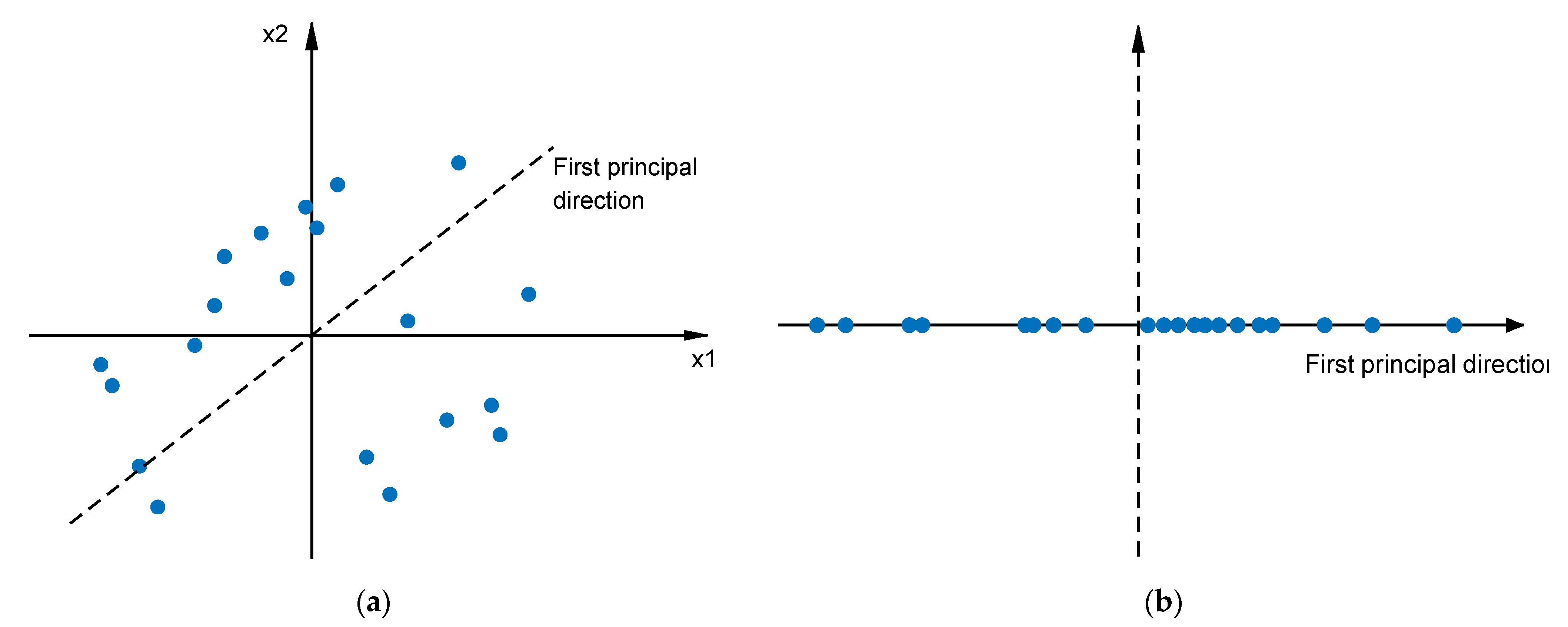[22] also proposed a new gradient enhancement alternative model method based on partial least squares, which greatly reduced the number of correlation parameters to enhance modeling efficiency. In addition, a new method based on principal component analysis (PCA) [23] has been proposed to approximate high-dimensional proxy models. It seeks the best linear combination coefficient that can be provided with the smallest error without using any integral. S. Marelli et al. [24] combined Kriging, polynomial chaos expansion and kernel PCA to prove and verify that the proposed high-dimensional proxy modeling method can effectively solve high-dimensional problems.

The above mentioned dimensionality reduction method reduces modeling time while ensuring that certain model accuracy requirements are met. After all, things have two sides. The improvement in modeling efficiency leads to a loss in accuracy to a certain extent. Therefore, how to improve modeling efficiency as much as possible while reducing the loss in accuracy requires further study.

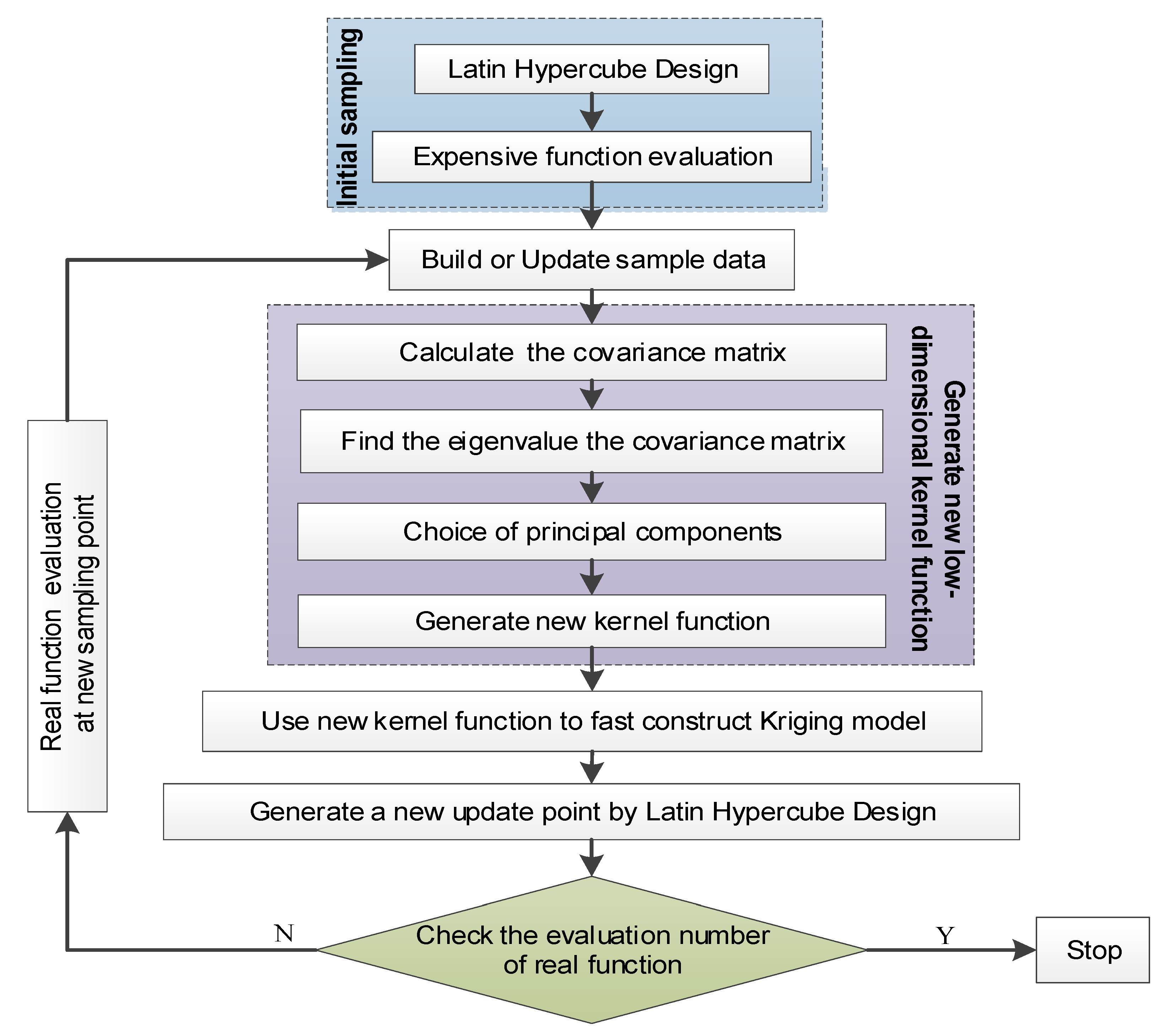
For this reason, a high-dimensional Kriging modeling method through principal component dimension reduction (HDKM-PCDR) is proposed. Through this method, the PCDR strategy can convert high-dimensional correlation parameters in the Kriging model into low-dimensional ones, which are used to reconstruct new correlation functions. The process of establishing correlation functions such as these can reduce the time consumption of correlation parameter optimization and correlation function matrix construction in the modeling process. Compared with the original Kriging method and the high-dimensional Kriging modeling method based on partial least squares, this method has better modeling efficiency under the premise of meeting certain accuracy requirements. In addition, the high-dimensional modeling method proposed in this article for the Kriging model will provide other researchers with new ideas and directions for the high-dimensional modeling research of surrogate models.

The remaining sections of this article are as follows. The second section introduces the characteristics of the Kriging model and its correlation parameter. The third section introduces the key issues of the proposed method and the specific implementation process in detail. In the fourth section, several high-dimensional benchmark functions and a simulation example are tested. Finally, conclusions are drawn and future research directions are envisioned.

2. Kriging Model

For experimental design sample $\mathbf{X}={[{\mathit{x}}_1,\dots ,{\mathit{x}}_{\mathrm{m}}]}^{\mathrm{T}}$($\mathbf{X}\in {\Re }^{m\times n}$) and corresponding objective $Y={[y_1, \dots , y_m]}^{\mathrm{T}}$($Y\in {\Re }^{m\times 1}$), the Kriging surrogate model combining polynomial regression and stochastic process can be expressed as

$$Y(\mathit{x})=F\mathit{\beta }+Z(\mathit{x})$$

(1)

where parameter $Y(\mathit{x})$ is a predicted function of interest. In this regression matrix $F$ with $F\in {\Re }^{m\times p}$, its elements are usually calculated by the first-order or second-order regression function of known observation points, and sometimes $F$ can also be a constant regression matrix. The weight β of the regression function is a p-dimensional column vector. The random process Z(x) with zero mean and variance can be stated as

$$\mathrm{E} [Z(\mathit{x})]=0,\hspace{1em}\mathrm{E} [Z\left(\mathit{x}\right)Z(\mathit{w}\left)\right]={\sigma }^{2}R(\mathit{\theta }, \mathit{\omega }, \mathit{x})$$

(2)

where θ is the correlation parameter and σ² is the process variance. For any two different observations ω and x, the spatial correlation kernel function R (θ, ω, x) is shown in Equation (3).

$$R(\mathit{\theta }, \mathit{\omega }, \mathit{x})={\displaystyle \prod _{i=1}^n{R}_i({\theta }_i, {\omega }_i-x_i)}$$

(3)

After determining the correlation among all sample points, the differentiability of the surface, the smoothness of the Kriging model and the influence of nearby points can be regulated by R (θ, ω, x). There are generally seven choices for the spatial correlation function. However, the most widely used is the Gaussian correlation model [25,26]. It can be expressed by

$$R_i\left({\theta }_i,w^k-x^k\right)=\exp \left(-{\theta }_i{\left|w^k-x^k\right|}^2\right)$$

(4)

According to the above analysis, the covariance correlation matrix R can be stated by Formula (5).

$$R_{m\times m}=\left[\begin{array}{cccc}R({\mathit{x}}_1,{\mathit{x}}_1)& R({\mathit{x}}_1,{\mathit{x}}_2)& \dots & R({\mathit{x}}_1,{\mathit{x}}_m)\\ R({\mathit{x}}_2,{\mathit{x}}_1)& R({\mathit{x}}_2,{\mathit{x}}_2)& \dots & R({\mathit{x}}_2,{\mathit{x}}_m)\\ ⋮ & ⋮ & \ddots & ⋮ \\ R({\mathit{x}}_m,{\mathit{x}}_1),& R({\mathit{x}}_m,{\mathit{x}}_2)& \dots & R({\mathit{x}}_m,{\mathit{x}}_m)\end{array}\right]$$

(5)

Due to unbiased estimation, the regression problem $F\mathit{\beta }\approx Y$ has a generalized least squares solution $\widehat{\mathit{\beta }}$ = ${\left(F^{\mathrm{T}}{R}^{-1}F\right)}^{-1}{F}^{\mathrm{T}}{R}^{-1}Y$ and a variance estimate ${\widehat{\sigma }}^2$=${\left(Y-F\widehat{\mathit{\beta }}\right)}^T{R}^{-1}\left(Y-F\widehat{\mathit{\beta }}\right)/m$.

As seen in Formula (2), process variance σ² and correlation parameter θ are closely related among matrix R. The unconstrained optimization problem of the maximum likelihood estimation in Equation (6) is maximized to determine optimal parameter θ.

$$-(m\ln {\sigma }^2+\ln \left|R\right|)/2$$

(6)

3. HDKM-PCDR Method

3.1. Use PCDR to Generate New Low-Dimensional Kernel Function

The mathematical theory of the principal component (PC) dimensionality reduction method is PCA, which is used here to reduce the dimensionality of the Kriging design variables. It uses the idea of dimensionality reduction. Under the premise of losing little potential function information, all indicators are transformed into several comprehensive ones by the multivariate statistical method. These comprehensive indicators after conversion are called principal components (PCs). Different linear combinations of original design variables can constitute different PCs. Under the condition that the PCs are independent of each other and meet the accuracy, the PCs after dimensionality reduction have greater advantages in modeling efficiency than the original variables. These are especially suitable for research into high-dimensional complex problems.

Suppose that the study of a certain problem involves n indicators denoted by $x^1,x^2,\dots ,x^n$. Therefore, the n-dimensional random vector $\mathit{x}={\left(x^1,x^2,\dots ,x^n\right)}^{\mathrm{T}}$ for any sampling point is formed by these n indicators. A new compound variable v in Equation (7) can be obtained by linear transformation of x; then, v is the PC we seek. If the first h (h <= n) PCs are selected, this is equivalent to reducing the number of indicators from n to h (that is, from n dimension to h dimension).

$$\{\begin{array}{c}{v}_1=u_{11}{x}^1+u_{12}{x}^2+\dots +u_{1n}{x}^n\\ v_2=u_{21}{x}^1+u_{22}{x}^2+\dots +u_{2n}{x}^n\\ \dots \dots \\ v_n=u_{n1}{x}^1+u_{n2}{x}^2+\dots +u_{nn}{x}^n\end{array}$$

(7)

The greater the variance in the principal component v_i, the greater the amount of original data information carried. We always hope that the PCs ($z_i={\mathit{u}}_i^{\mathrm{T}}x$) are independent of each other and have the largest possible variance. However, in fact, if there is no restriction on ${\mathit{u}}_i$, it may make the variance increase arbitrarily; the problem will therefore become meaningless. For this reason, linear transformation needs to follow the following principles:

Principle 1. 

Ensure that${\mathit{u}}_i^{\mathrm{T}}{\mathit{u}}_i$is equal to 1, that is,$u_{i1}^2+u_{i2}^2+\dots +u_{in}^2=1 \left(i=1,2,\dots ,n\right)$;

Principle 2. 

Make$v_i$and$v_j$irrelevant, that is$\mathrm{cov}(v_i,v_j)=0, i\ne j; i,j=1,2,\dots ,n$;

Principle 3. 

Ensure that$v_1$is the one with the largest variance among all linear combinations of$x^1,x^2,\dots ,x^n$that satisfy principle 1;$v_2$is the one with the largest variance among all linear combinations of$x^1,x^2,\dots ,x^n$when it is not correlated with$v_1$; follow this rule, etc.,$v_n$is the one with the largest variance among all linear combinations of$x^1,x^2,\dots ,x^n$when it is not correlated with$v_1,v_2,\dots ,v_{n-1}$.

Based on the above three principles, the determined composite variable $v_1,v_2,\dots ,v_n$ is the first to the nth PC of the original variable. And the variances of the composite variable $v_1,v_2,\dots ,v_n$ are arranged in descending order.

According to the above analysis, the specific calculation process of the PCDR method is described as follows:

• Step 1: Calculation of the covariance matrix. Suppose and offer the covariance matrix of the sample data is $\sum ={\sigma }^{2}R={\left(s_{ij}\right)}_{n\times n}$.
• Step 2: Find the eigenvalue ${\lambda }_i$ of $\sum$ and the corresponding unit eigenvector ${\mathit{u}}_i$, and arrange the eigenvalues ${\lambda }_i$ of the covariance matrix $\sum$ as ${\lambda }_1,{\lambda }_2,\dots ,{\lambda }_n \left({\lambda }_1\ge {\lambda }_2\dots {\lambda }_n\right)$ in order of magnitude, and the corresponding unit eigenvectors ${\mathit{u}}_1,{\mathit{u}}_2,\dots ,{\mathit{u}}_d$ are the coefficient vectors of the principal component $v_i\left( i=1,2,\dots ,n\right)$, respectively.
• Step 3: Choice of PCs. The variance value of each PC $v_i$ is equal to the corresponding ${\lambda }_i$ [27]. Therefore, the contribution rate $C{R}_i$ of the eigenvalue (or variance) is used to reflect the amount of information; that is, $C{R}_i={\lambda }_i/{\displaystyle \sum _{i=1}^n{\lambda }_i}$.

Then, the value h can be determined by the cumulative contribution rate of variance in Equation (8).

$$CR\left(h\right)={\displaystyle \sum _{i=1}^h{\lambda }_i}/{\displaystyle \sum _{i=1}^n{\lambda }_i}$$

(8)

When the cumulative contribution rate is greater than 80%, we believe that the PC can reflect the characteristic of the original variable to a certain extent, and the corresponding parameter h is the final selected principal component number:

• Step 4: Determine a new conversion matrix according to the known sample data and using the formula $z_i=u_{i1}{x}^1+u_{i2}{x}^2+\dots +u_{id}{x}^d$($i=1,\dots ,h$) to calculate the value of the h PCs; meanwhile, the n*h transformation matrix is obtained. This matrix is used as a weight to replace Formula (3) and recalculate the new kernel function in a more efficient way.
• Step 5: Generate new kernel function. First, the linear mapping expression is defined and shown in Equation (9).

$$\begin{array}{l}{F}_l:B\to B\\ \mathit{x}\mapsto \left[u_l^1{x}_1,\dots ,u_l^n{x}_n\right] l=1,\dots ,h \end{array}$$

(9)

where B is a hypercube belonging to ${\Re }^d$ and is represented by the product of the space interval in each direction. The corresponding kernel function is expressed as

$$R_l\left({\theta }_l,F_l\left(x\right),F_l\left(\mathit{w}\right)\right)={\displaystyle \prod _{i=1}^n\exp \left(-{\theta }_l{\left|u_l^i{w}^i-u_l^i{x}^i\right|}^2\right)}$$

(10)

Finally, through the tensor product of h kernel functions, a new kernel function based on Kriging and PCA (KPCA), as shown in Equation (11), can be generated. For new spatial correlation kernel function, we can use the reduced-dimensional Formula (11) to replace the high-dimensional Formula (3) so as to improve the modeling efficiency of the Kriging model.

$$\begin{array}{ll}{R}_{\mathrm{KPCA}}\left(\mathit{x},\mathit{w}\right)& ={\displaystyle \prod _{l=1}^h{R}_l\left(F_l\left(\mathit{x}\right),F_l\left(\mathit{w}\right)\right)}\\ & ={\displaystyle \prod _{l=1}^h{\displaystyle \prod _{i=1}^n\exp \left(-{\theta }_l{\left|u_l^i{w}^i-u_l^i{x}^i\right|}^2\right)}}, \forall \mathit{x},\mathit{w}\in B \end{array}$$

(11)

Next, take the two-dimensional GP function as an example to describe the dimensionality reduction process of the PCDR more clearly. First, use the LHD sampling method to randomly select 20 sample points, which are shown in Figure 1a. Next, calculate the covariance matrix of the sample points and use the eigenvector with the largest eigenvalue in the matrix as the first principal direction (the dotted line in Figure 1a). The first principal direction is essentially the coefficient in the linear transformation vector. In this way, the linear transformation of Equation (7) maps the original data points to the direction of the first principal component (as shown in Figure 1b). Thus far, the first four steps in the PCDR method are completed. The fifth step is to calculate a new spatial kernel function through the data points after dimensionality reduction, and then complete the low-dimensional Kriging modeling.

3.2. Specific Implementation of HDKM-PCDR Method

The process of the HDKM-PCDR is shown and stated in detail in Figure 2. Additionally, its specific implementation steps are presented as follows:

• Step 1: Initial sampling. LHD (Latin Hypercube Design) method [28] is employed to generate the initial sample points. To facilitate comparison with other methods, different initial sampling points will be selected for different real function evaluation times.
• Step 2: Build or update sample data. If the sampling data are obtained by the initial LHD method, we will establish the sample data set {S, Y} for the first time. If a new sampling point (s, y) is generated by LHD in the optimization process, we will update the sample data set, i.e., [S, s] → S, [Y, y] → Y.
• Step 3: Generate new low-dimensional kernel function.
• Step 4: Use new kernel function to rapidly construct the Kriging model.
• Step 5: Generate a new candidate point by Latin Hypercube Design.
• Step 6: Check the evaluation number of the expensive function.
• Step 7: Expensive function evaluation at the new update point.

4. Numerical Test

The KPLS method was proposed by Bouhlel et al. in 2016, and [29,30] demonstrated that the KPLS method is highly effective at solving high-dimensional problems. The KPLS combining PLS (partial least squares) technique and Kriging model uses the least squares dimensionality reduction method in the process of establishing the Kriging model, which reduces the number of hyper-parameter calculations of the model to be consistent with the number of PCs retained by the PLS, thereby accelerating the construction of the Kriging model. For this reason, we can prove the effectiveness of HDKM-PCDR by comparing HDKM-PCDR with the KPLS method. If the test result of HDKM-PCDR is better, it can prove the effectiveness of the HDKM-PCDR method. In addition, Kriging is also used as a comparison method to verify the applicability of the HDKM-PCDR method for solving high-dimensional problems.

To compare HDKM-PCDR and KPLS methods in a better and more detailed way, this work keeps the number of PCs retained in the two methods consistent. The modeling time and modeling error of the two methods are tested when one principal component, two PCs and three PCs are retained, respectively.

According to the characteristics of the function’s multimodality, the complexity degree (the number of valleys or ridges) and the level of dimensionality, the 20-dimensional Griewank function, the 40-dimensional SUR function, the 60-dimensional DixonPrice function and the 80-dimensional Michalewicz function shown below are chosen as the Benchmark functions.

Griewank function:

$$y(\mathit{x})={\displaystyle \sum _{i=1}^{20}\frac{x_i^2}{4000}}-{\displaystyle \prod _{i=1}^{20}\cos (\frac{x_i}{\sqrt{i}})}+1 -600\le x_i\le 600$$

(12)

SUR function:

$$y(\mathit{x})={(x_1-1)}^2+{(x_{40}-1)}^2+40{\displaystyle \sum _{i=1}^{39}(40-i)}{(x_i^2-x_{i+1})}^2 -3\le x_i\le 2$$

(13)

DixonPrice function:

$$y(\mathit{x})={(x_1-1)}^2+{\displaystyle \sum _{i=2}^{60}i}{(2x_i^2-x_{i-1})}^2 -10\le x_i\le 10$$

(14)

Michalewicz function:

$$y(\mathit{x})=-{\displaystyle \sum _{i=1}^{80}\sin (x_i)}{\sin }^{160}(\frac{i{x}_i^2}{\pi }) 0\le x_i\le \pi$$

(15)

For each test function, it is tested in two cases. The first case is to obtain 10 initial sampling points through LHD, and then new sampling points will be added until the total number of samples reaches 100. The second case is to obtain 20 initial sampling points; when the total number of samples reaches 200, stop the HDKM-PCDR method. The total number of sampling points here is reflected in

Table 1. Test results on time and RMSE for the Griewank function.

Test Method	100 Sample Points		200 Sample Points
	Time (s)	RMSE	Time (s)	RMSE
Kriging	7.5573	11.9916	74.1562	8.6062
HDKM-PCDR-1	0.7652	10.3085	6.5901	6.6526
KPLS-1	0.8119	10.1789	6.6855	6.8414
HDKM-PCDR-2	1.3173	9.6095	13.7230	5.4336
KPLS-2	1.3510	9.9492	13.7983	6.8227
HDKM-PCDR-3	2.5512	9.3348	30.8119	5.4700
KPLS-3	2.7733	9.8196	30.9308	6.7632

,

Table 2. Test results on time and RMSE for the SUR function.

Test Method	100 Sample Points		200 Sample Points
	Time (s)	RMSE	Time (s)	RMSE
Kriging	18.2212	1.3791 × 104	216.5188	1.1123 × 104
HDKM-PCDR-1	1.2272	1.2820 × 104	12.8934	8.8252 × 103
KPLS-1	1.9691	1.2301 × 104	14.1654	7.0127 × 103
HDKM-PCDR-2	2.2761	1.1949 × 104	23.5094	7.6304 × 103
KPLS-2	2.3510	1.2795 × 104	24.1808	8.4033 × 103
HDKM-PCDR-3	4.1168	1.2322 × 104	55.3962	8. 3669 × 103
KPLS-3	4.7523	1.2576 × 104	55.7409	8. 7498 × 103

,

Table 3. Test results on time and RMSE of the DixonPrice function.

Test Method	100 Sample Points		200 Sample Points
	Time (s)	RMSE	Time (s)	RMSE
Kriging	61.4766	2.8969 × 105	664.3026	2.1001 × 105
HDKM-PCDR-1	2.9292	2.8021 × 105	24.3048	1.9415 × 105
KPLS-1	2.8138	2.8041 × 105	25.0655	1.9264 × 105
HDKM-PCDR-2	4.8741	2.7954 × 105	54.7819	1.8945 × 105
KPLS-2	5.9279	2.7961 × 105	56.8854	1.8879 × 105
HDKM-PCDR-3	15.2038	2.6808 × 105	126.8160	1.8643 × 105
KPLS-3	13.6838	2.6488 × 105	137.2857	1.8654 × 105

and

Table 4. Time and RMSE of the Michalewicz function.

Test Method	100 Sample Points		200 Sample Points
	Time (s)	RMSE	Time (s)	RMSE
Kriging	126.6239	0.1296	1289.3620	0.0925
HDKM-PCDR-1	3.4028	0.1276	25.9314	0.0916
KPLS-1	3.6180	0.1276	26.9781	0.0918
HDKM-PCDR-2	4.7722	0.1248	53.1837	0.0920
KPLS-2	5.0228	0.1264	53.8481	0.0923
HDKM-PCDR-3	19.3122	0.1241	184.6957	0.0915
KPLS-3	32.3037	0.1238	285.4663	0.0908

. For the test in each case, in order to reflect the robustness and effectiveness of the HDKM-PCDR, the average value of ten repeated runs is taken as the final test result.

The results of the time consumption and modeling error (RMSE-Root Mean Square Error) of the four test functions are shown in Table 1, Table 2, Table 3 and Table 4. The time is the total modeling time spent during the whole sampling process for all sample points. The RMSE in these tables can be obtained by using “leave one out cross” validation [31]. The concrete expression of RMSE is shown in Equation (12). Here, parameter k represents the number of samples in the current data. If the Kriging model is used to estimate the variance of point ${\mathit{x}}_i$, we first need to reconstruct the Kriging model with the remaining k-1 sampling points, except for point ${\mathit{x}}_i$. Then, calculate the estimated variance ${\widehat{s}}_i^2$ of point ${\mathit{x}}_i$ by using the newly built Kriging model and Formula (8). After repeating k times to complete the variance estimation of these k sampling points, the average value can be calculated to obtain the RMSE with Equation (12).

$$\mathrm{RMSE}=\frac{1}{k}\sqrt{{\displaystyle \sum _{i=1}^k{\widehat{s}}_i^2}}$$

(16)

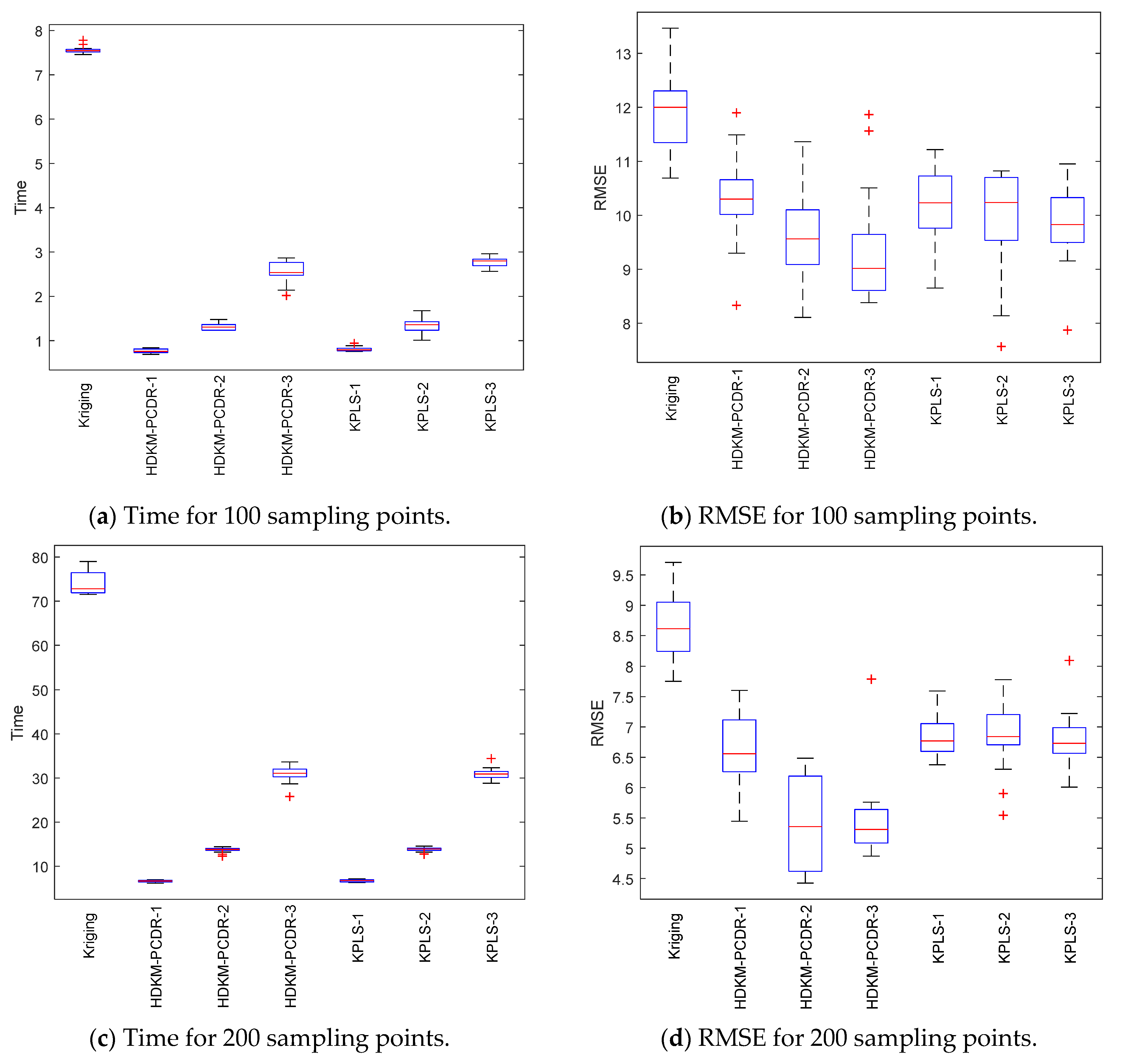
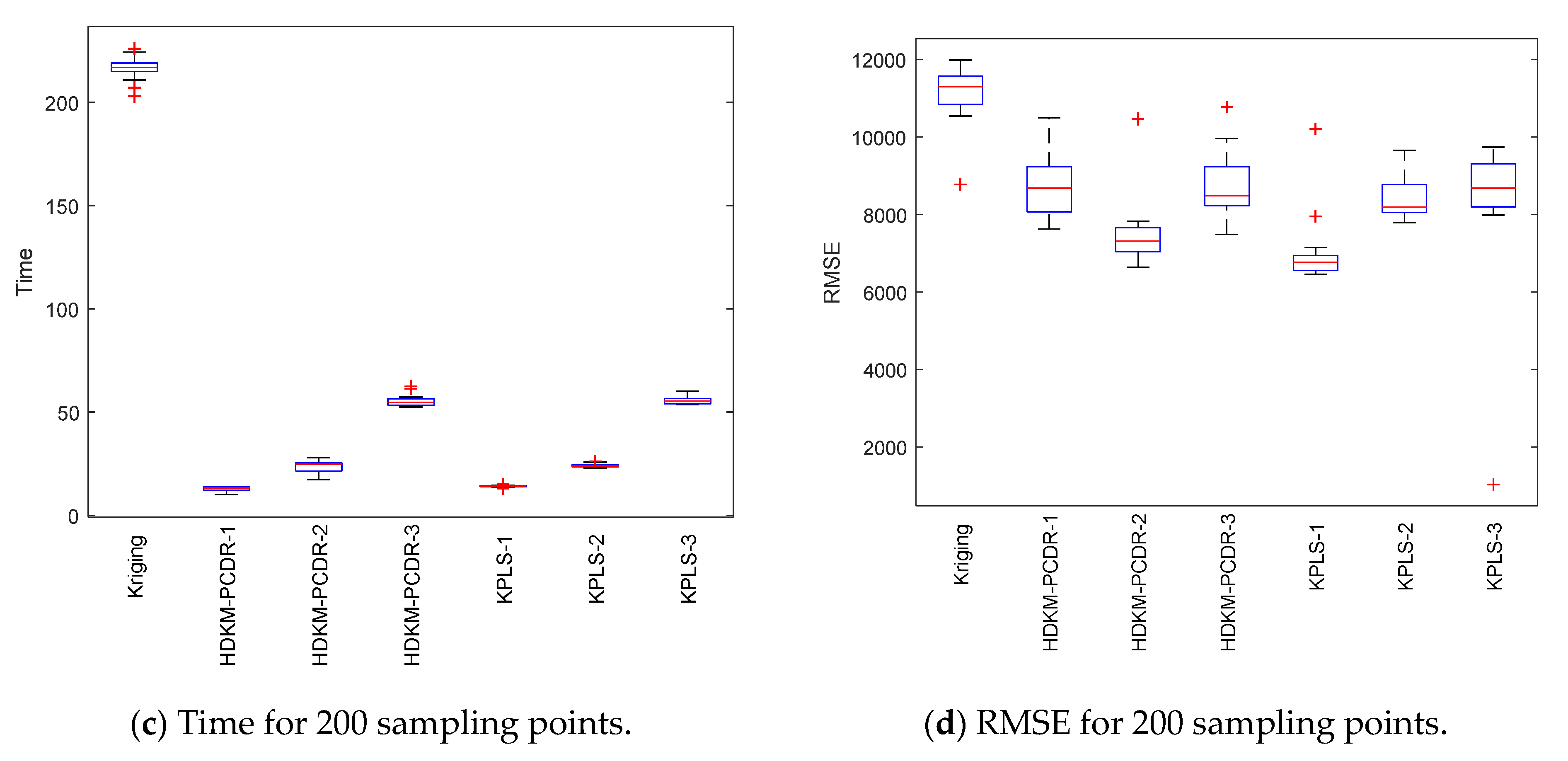
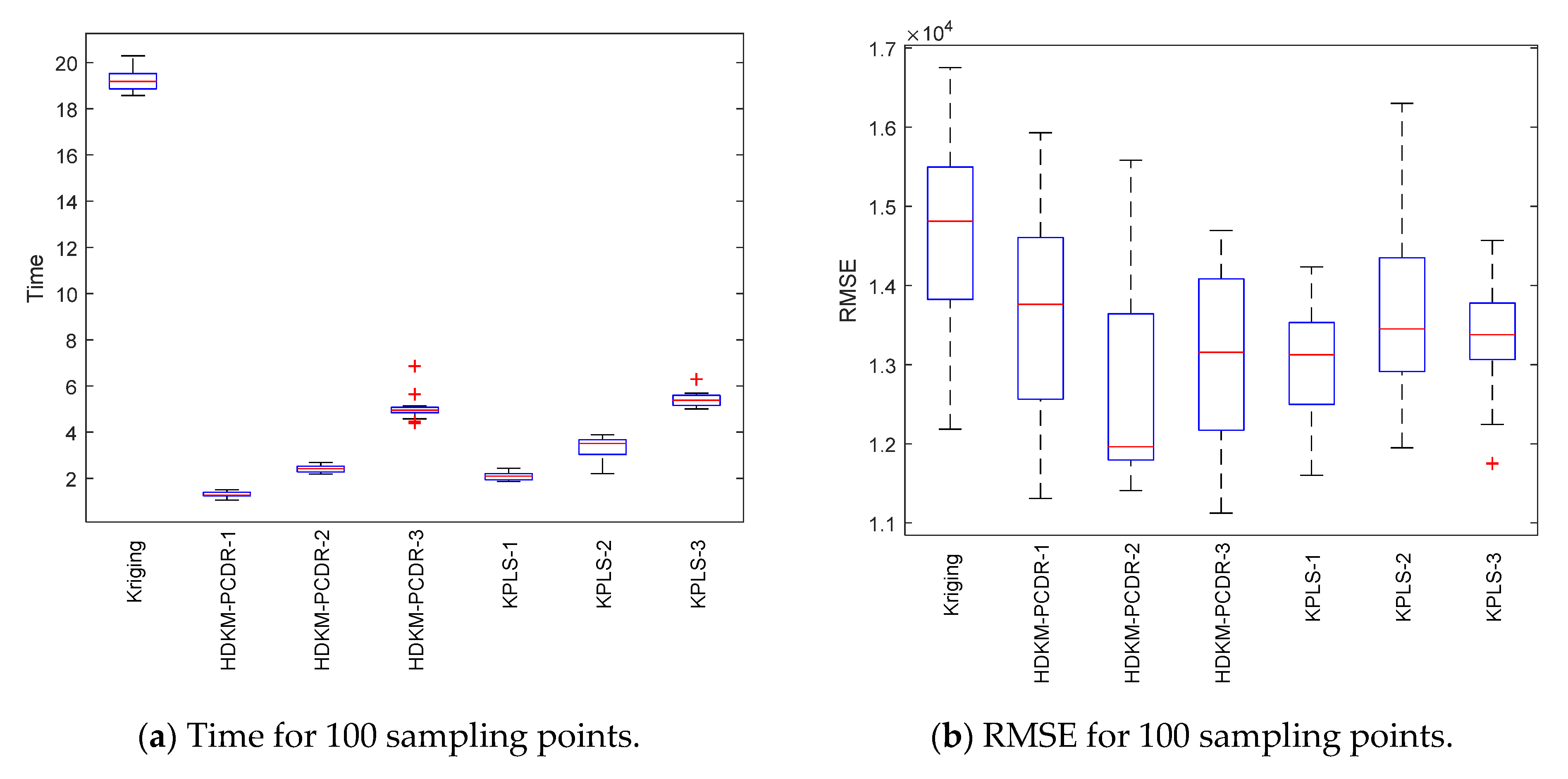
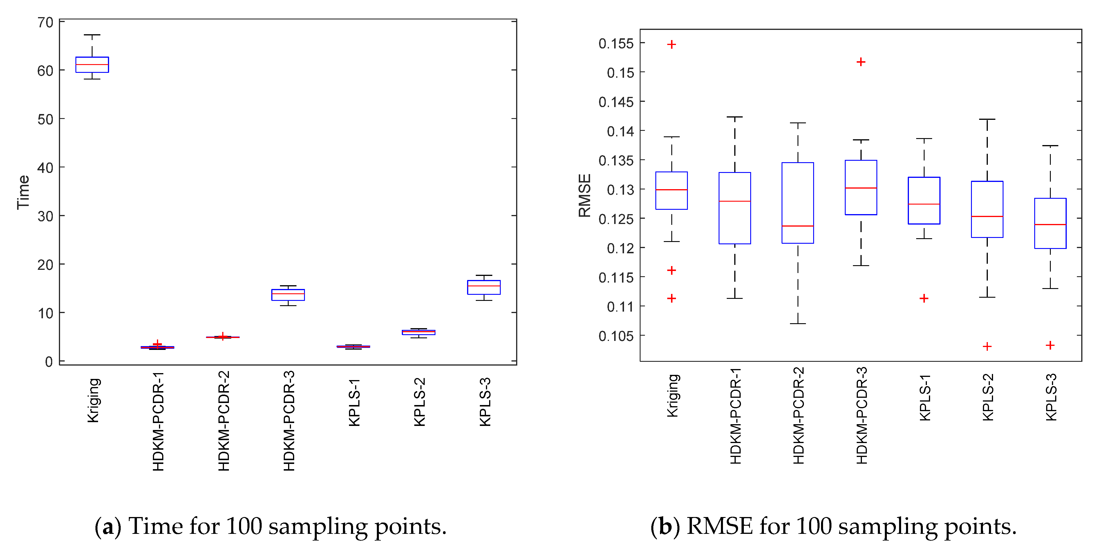
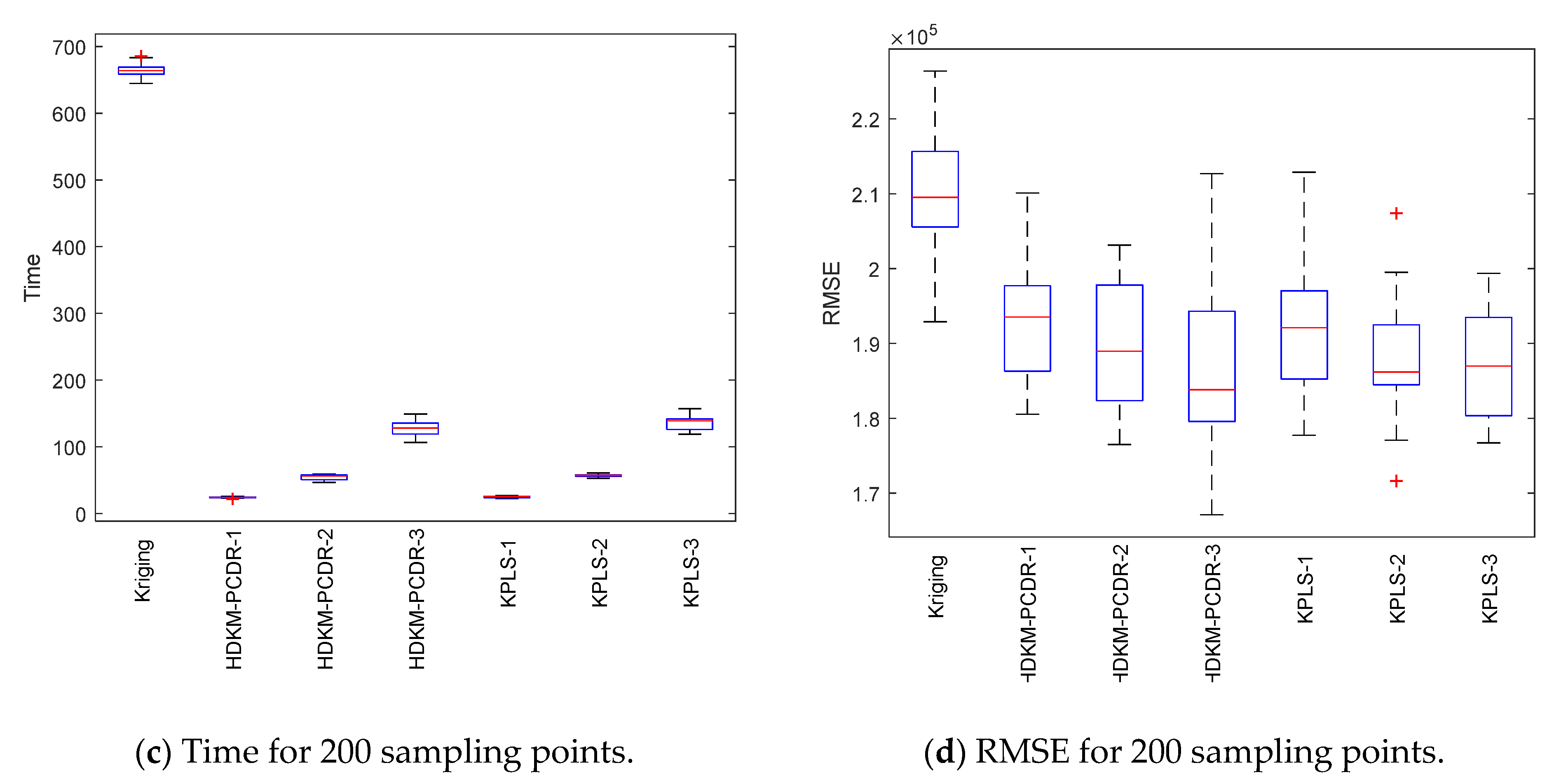
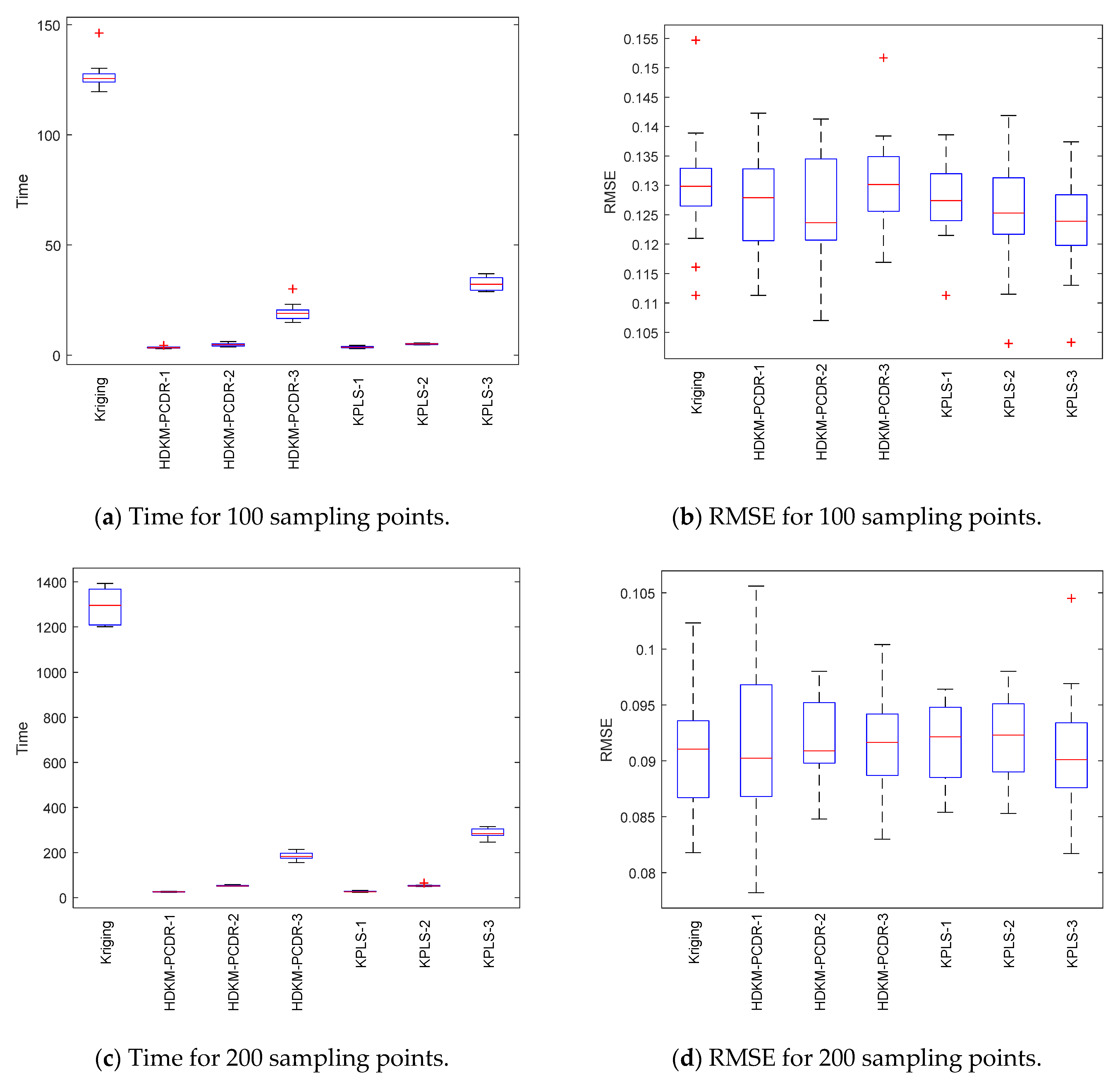
Under the condition of different sample points, box plots of 10 test results of each test function are, respectively, shown in Figure 3, Figure 4, Figure 5 and Figure 6 to further demonstrate the stability and effectiveness of the HDKM-PCDR method, as well as to express it intuitively.

First, let us take a look at the modeling time test results of the algorithms from subgraphs (a) and (c) in Figure 3, Figure 4, Figure 5 and Figure 6. Compared with ordinary Kriging and KPLS methods, from the median (red solid line) of the time box plots and the size (the area formed by the upper quartile and the lower quartile) of the box, the median line value shown by the proposed method is the lowest, and the frame area is also the smallest. In addition, it has fewer outliers. For example, in the Griewank function test of 200 sampling points, the HDKM-PCDR-3 method and the KPLS-3 method have abnormal points. However, the abnormal points generated by the HDKM-PCDR-3 method are located below the box plot, while the abnormal point of KPLS-3 is located above the box plot. This shows that the time consumed by HDKM-PCDR-3 in the ten test cycles has a smaller value in a certain test, while KPLS-3 has a larger value. Therefore, the proposed method has the shortest modeling time in the process of each test, and the fluctuation of the time spent in these ten modeling times is not large. These test results show that the HDKM-PCDR modeling method has better stability and efficiency.

The modeling time and model accuracy in each of the four tables are the average of the results obtained after ten runs of each benchmark function. All tests were performed in Matlab2018a by a Lenovo machine equipped with an i5–4590 3.3 GHz CPU and 4 GB RAM. As expected, for these four benchmark functions, the HDKM-PCDR method and the KPLS method under the dimensionality reduction condition use 100 and 200 sampling points to establish the Kriging model. The corresponding time spent and the approximate accuracy of the model are better than the Kriging method without direct dimensionality reduction. For the HDKM-PCDR method and the KPLS using the idea of dimensionality reduction, the modeling time shown by the HDKM-PCDR-n (n = 1, 2, 3) method stays ahead of the KPLS-n (n = 1, 2, 3) method under the condition of reducing the same dimensions. For Griewank, SUR and DixonPrice functions, although the modeling time of the proposed method is slightly lower than that of KPLS, the total modeling time of the two methods is not much different. For the more complex Michalewicz function, the HDKM-PCDR-3 method takes only a little more than half of the time of the KPLS-3 method, which also shows that the HDKM-PCDR method has higher efficiency in dealing with multi-dimensional and multi-peak complex problems. In terms of model accuracy, except for the KPLS-1 method at 100 points, the test results of Griewank function using the proposed method perform best. Other than the KPLS-1 method in the case of 100 points and 200 points, the RMSE obtained by the HDKM-PCDR method to test the SUR function meets the high accuracy requirements. For the DixonPrice and Michalewicz functions, the two methods are evenly matched, and both have advantages. However, considering modeling time and model accuracy, the proposed method is slightly better.

Next, let us look at the test results of the modeling accuracy of the algorithm from sub-graphs (b) and (d) in Figure 3, Figure 4, Figure 5 and Figure 6. Theoretically speaking, the RMSE (model accuracy) of the ordinary Kriging method without dimensionality reduction should be the best. However, as can be seen from subgraphs (b) and (d), the fact is just the opposite. Judging from the median RMSE in the Griewank function test results, the HDKM-PCDR performs better than the KPLS. For SUR function, in addition to KPLS-1, the accuracy results in other cases are still slightly better than the proposed method. For the DixonPrice function and the Michalewicz function, these two dimensionality reduction methods are evenly matched, and each has its own merits. However, KPLS-2 and KPLS-3 both showed better performance of abnormal points in some test functions, which is better than the proposed method. However, in general, the proposed method is still stronger than KPLS, and can ensure that the accuracy of the problem after dimensionality reduction meets certain requirements.

In summary, the following conclusions can be drawn for all the above test results: (1) Compared to the non-dimensionality reduction Kriging method, regardless of the modeling time and the accuracy of the model, the HDKM-PCDR method and the KPLS method using dimensionality reduction have been improved. (2) The modeling time of the HDKM-PCDR method is almost always shorter than that of the KPLS method while retaining the same number of PCs. Additionally, with the increase in the dimension and the number of sample points, the efficiency advantage of the HDKM-PCDR method becomes more and more obvious. The main reason for this is that the proposed method reduces the size of the hyperparameter correlation matrix in the Kriging model, which is equivalent to simplifying the internal structure of the Kriging model, thereby improving the efficiency of Kriging modeling. (3) However, in terms of modeling accuracy, for different functions, the proposed method and the KPLS method have their own advantages in accuracy. For example, HDKM-PCDR’s test results of Griewank function show that its modeling accuracy is higher. The results of the proposed method and the KPLS method for the other three benchmark functions are basically evenly divided. The main reason is explained as follows: the reduction in the proposed method is mainly for the reduction in the dimensions of the related hyperparameters, which directly leads to the reduction in the correlation matrix, while the KPLS method also considers the PLS method and the Kriging estimation of the sampling points. These two different reduction methods consider different angles for the reduction problem, resulting in approximate accuracy sometimes being better than KPLS; sometimes, KPLS is better than the proposed method, but the overall accuracy values are not much different and are even close. (4) In some special circumstances, when the dimensionality of the problem is higher after dimensionality reduction, the model’s accuracy will decrease instead. For example, when the Michalewicz function is tested at 200 sampling points, it appears that the accuracy of HDKM-PCDR-1 and KPLS-1 are better than HDKM-PCDR-2 and KPLS-2. The reason for this result may be that the sample point contains a large amount of information when it is reduced to one-dimensional data. In other words, the weight of the function on a certain dimensional variable is too large. However, this situation is rare seen in practice.

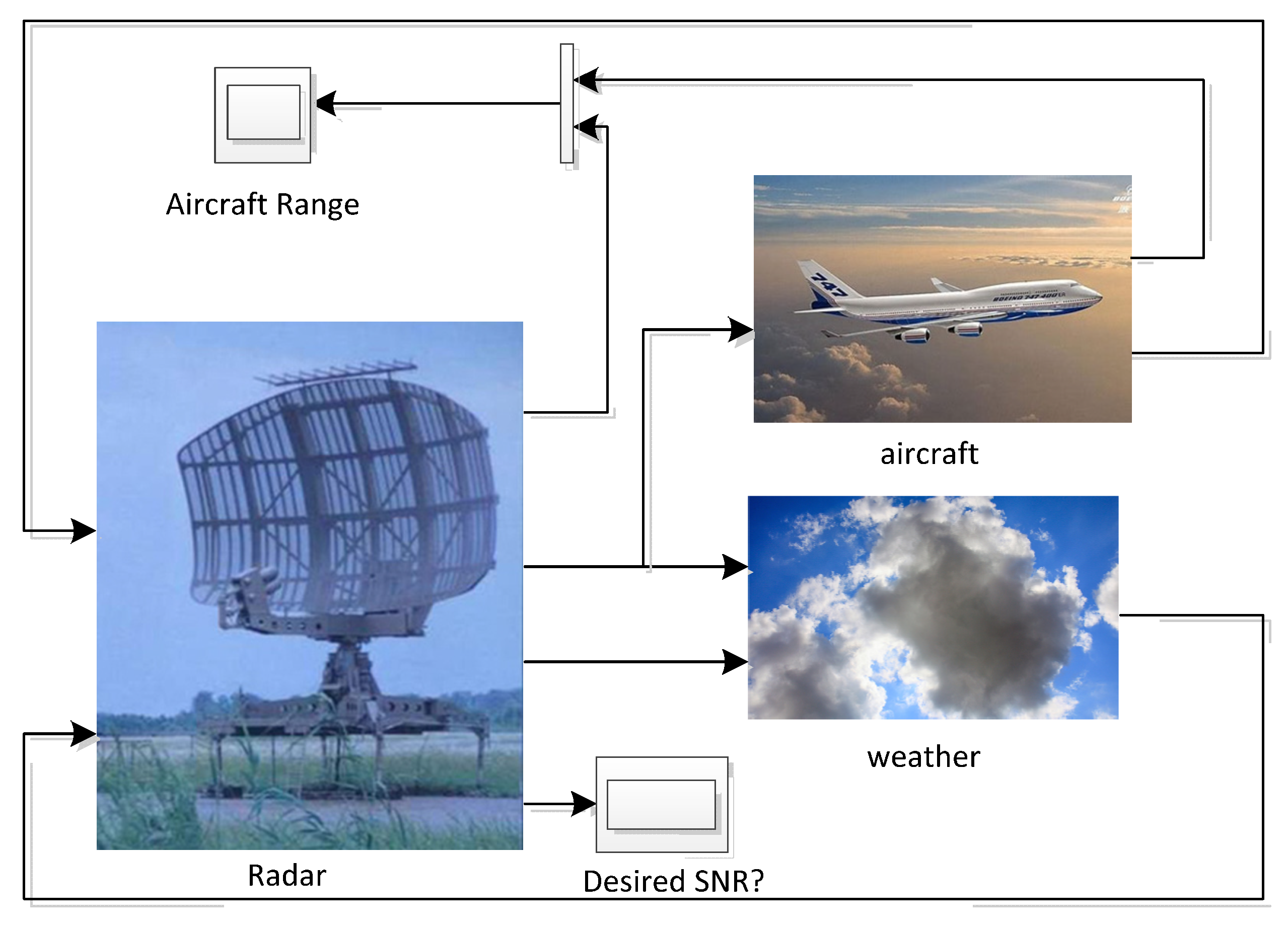
5. Air Traffic Control Radar Design

With the continuous and rapid development of China’s air traffic field, air traffic control technology has higher and higher requirements for the perception of future air traffic situations. In order to ensure the flight safety of aircraft and the normal operation of air traffic in real time, a radar detection system has been set up. This radar detection system can monitor the flight range of an aircraft in real time. In this case, unfortunate events such as missing aircraft can be avoided.

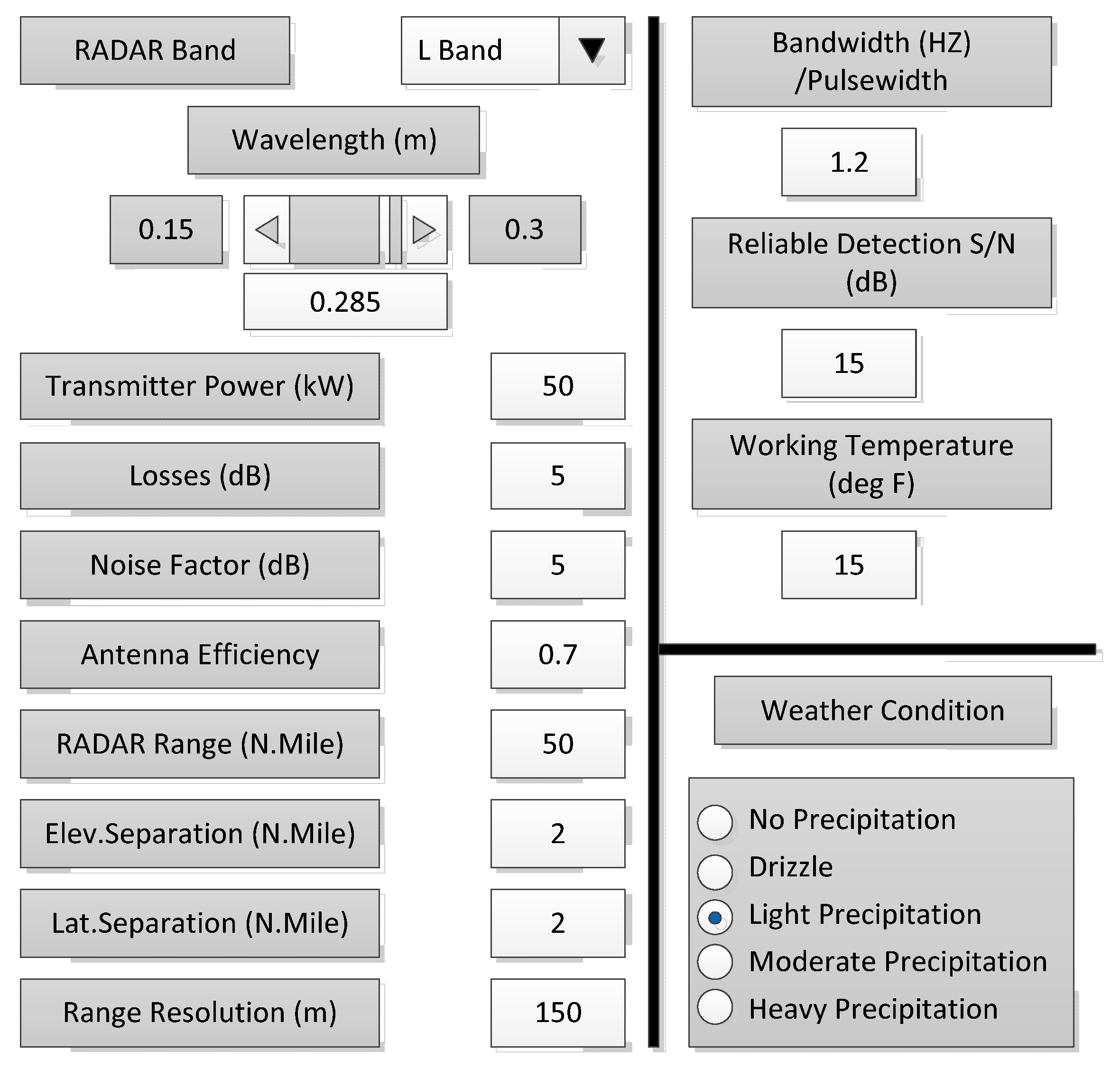
In order to better design the above air traffic control radar, we simulated an air traffic control (ATC) radar design through Simulink simulation software in MATLAB. The simulation model can be divided into three main subsystems: radar, aircraft and weather. The specific air traffic control model diagram is shown in Figure 7. The air traffic control radar simulation system designed in this paper introduces real-time data such as flight information, radar signals, weather forecast, aircraft resistance and flight mileage as simulation parameters in the simulation process. In order to make the parameters of the radar system design easier to change and easier to determine their values, this model provides a GUI (see Figure 8). The parameters of radar and weather can be changed through the GUI. The effect of different parameters can be seen on the oscilloscope screen during simulation. The oscilloscope screen shows the actual range of the aircraft and the change over time in the aircraft’s range estimated by radar under certain parameter settings.

This paper takes the design variables as the parameter settings of the air traffic control radar design simulation system, so that the simulation results can be obtained by Simulink. Since the simulation result changes with time, the maximum range of radar detection is taken as the simulation result and output to the MATLAB workspace. Based on the simulation results and the HDKM-PCDR method, one, two and three principal components are retained to construct the Kriging model, and the modeling time and modeling error in the three cases are recorded. In addition, the Kriging model was directly established with the data obtained from the simulation, and modeling time and modeling error were also recorded.

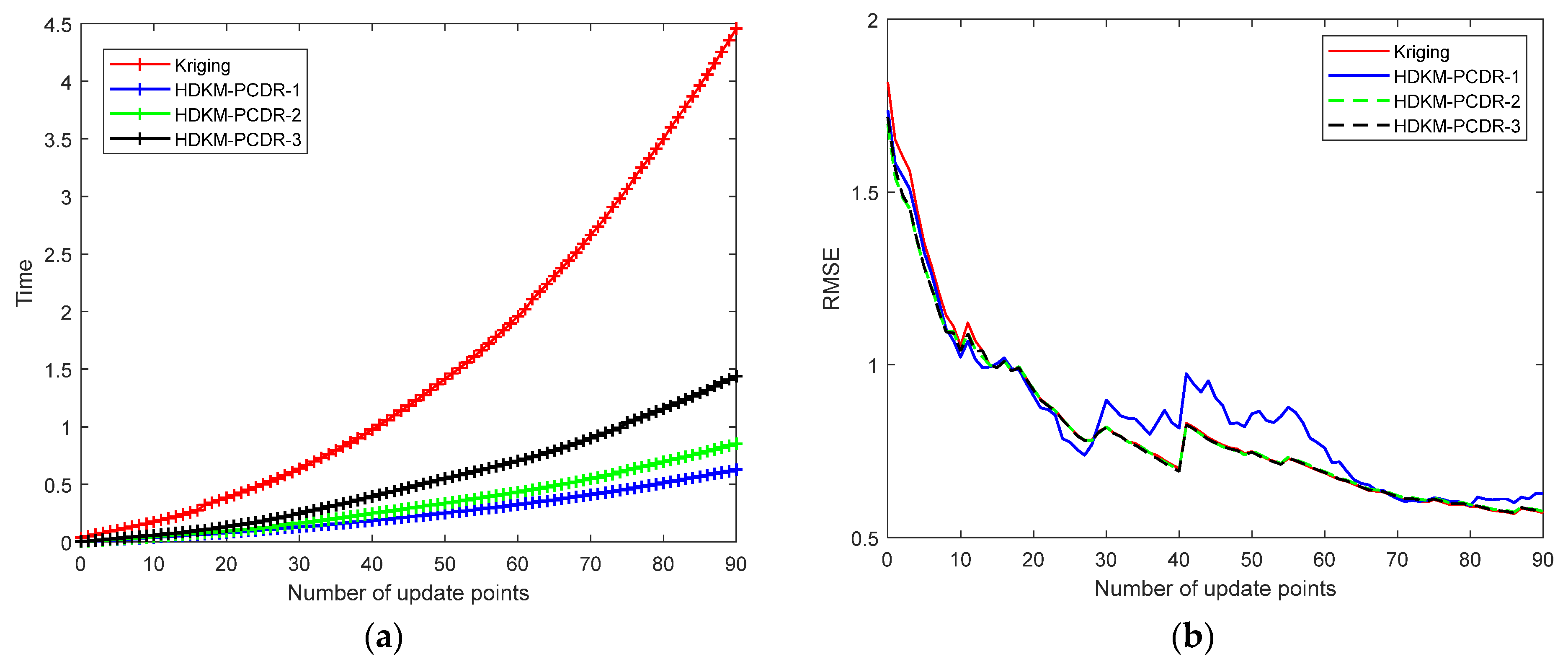
Figure 9 shows the results of modeling time and modeling error in a modeling process. In order to better compare the time for the HDKM-PCDR method to establish Kriging and to directly establish the Kriging model, the time in Figure 7 has removed the time used for simulation. In this modeling process, there are 10 initial sample points, and the corresponding expensive estimates of the sample points are obtained through simulation. The Kriging model is established by the HDKM-PCDR method, and the modeling time at this time (excluding time for simulation estimation) is recorded as a first-time value. In each iteration, a sample point is added, and the corresponding expensive estimate is simulated; modeling time at this time (excluding the time for the simulation estimate) is recorded as a time value. Repeat the iterative process until final sample number is 100, and then stop the iterative process.

The following two conclusions can be drawn from the figure: (a) It can be seen from the figure that, as the number of sample points increases, the time required for HDKM-PCDR and Kriging to build a model gradually increases. However, with the increase in the number of sample points, the time required to directly establish the Kriging model is greater than the time required to establish the model of HDKM-PCDR. In the end, the time difference is 8 times, 6 times and 3.2 times, respectively. (b) It can be seen from the figure that the modeling error is gradually reduced as the number of sample points increases. The modeling error of the HDKM-PCDR-1 method is unstable and large, but it is not much different from the modeling error of the Kriging method. The modeling errors of the HDKM-PCDR-2 and HDKM-PCDR-3 methods are very close to those of the Kriging method. In summary, the HDKM-PCDR method can improve the modeling efficiency of the Kriging model when the modeling accuracy loss is small.

6. Conclusions

The complexity of engineering problems causes calculating time to be expensive. Therefore, the Kriging surrogate model is used to reduce this burden. However, when using the Kriging model to approximate high-dimensional problems, the modeling process is also time consuming. The most time is spent during the inversion of the covariance correlation matrix and the solving of the Kriging correlation parameter. To this end, a high-dimensional Kriging modeling method through principal component dimension reduction (HDKM-PCDR) is proposed. In this method, the PCDR way of considering design variables and correlation parameters can convert the high-dimensional correlation parameter in Kriging into a low-dimensional one, which is used to reconstruct a new correlation function. In this way, it will reduce the time spent optimizing correlation parameters and constructing the correlation function matrix in the Kriging modeling process. Compared with the original Kriging method and the high-dimensional Kriging modeling based on partial least squares, the proposed method has better modeling efficiency while meeting certain accuracy requirements.

When dealing with high-dimensional problems, the proposed method has certain deficiencies in relation to model accuracy. In principal component dimensionality reduction, it is necessary to ensure that the cumulative contribution rate of the first few principal components extracted reaches a higher level (that is, the variable after dimensionality reduction has a higher amount of information). In this case, when the correlation between the original design variables is weak, too many principal components may be selected, which is not conducive to improvements in Kriging modeling efficiency. In future research, we will further explore new sampling strategies by combining factors such as prediction target, variance, and distance. In this way, more promising sampling points can be obtained to improve the model accuracy.