Article

Trochoidal Milling Path with Variable Feed. Application to the Machining of a Ti-6Al-4V Part

by
César García-Hernández
1,*,
Juan-José Garde-Barace
2,
Juan-Jesús Valdivia-Sánchez
2,
Pedro Ubieto-Artur
1,
José-Antonio Bueno-Pérez
3,
Basilio Cano-Álvarez
4,
Miguel-Ángel Alcázar-Sánchez
4,
Francisco Valdivia-Calvo
2,
Rubén Ponz-Cuenca
5,
José-Luis Huertas-Talón
1,2 and
Panagiotis Kyratsis
6
1
Department of Design and Manufacturing Engineering, University of Zaragoza, 50018 Zaragoza, Spain
2
CPIFP “Corona de Aragón”, 50009 Zaragoza, Spain
3
IES “Jaume Huguet”, 43800 Tarragona, Spain
4
CIFP “Virgen de Gracia”, 13500 Ciudad Real, Spain
5
Marena, S.L., 50171 Zaragoza, Spain
6
Department of Industrial Design Engineering, University of Western Macedonia, GR 50100 Kozani, Greece
*
Author to whom correspondence should be addressed.
Mathematics 2021, 9(21), 2701; https://doi.org/10.3390/math9212701
Submission received: 27 September 2021 / Revised: 18 October 2021 / Accepted: 22 October 2021 / Published: 25 October 2021
(This article belongs to the Special Issue Modeling and Simulation in Engineering)

Abstract

:
Trochoidal milling is a well-stablished machining strategy which still allows for the introduction of new approaches. This strategy can be applied to any kind of material, although it is usually associated to advanced materials, such as titanium and nickel alloys. This study is based on the adaptation of the feed speed of a milling tool with Ti-6Al-4V, so the chip width can be maintained constant without modifying the path geometry. A singularity in the experimental stage was to mill an Archimedes spiral groove instead of the conventional straight grooves. This made it possible to obtain a concave wall as well as a convex one and to optimize the amount of material used. The time efficiency compared to a constant feed, was slightly superior to 20%, reducing tool wear also. These techniques require milling machines with high mechanical and kinematic performance, as well as the absence of clearance between joints and a high acceleration capacity.

1. Introduction

The main objective of trochoidal milling is to use all the effective tool length in order to make the cut [1]. The cutting force on the tool depends on the chip section and produces the tool flection; furthermore, the cutting power is proportional to the cutting force. A similar cutting force can appear due to the elimination of a large chip width ae and a small axial depth of cut ap, or the removal of a small chip width and a large axial cut, Figure 1.
The force application point on the right of Figure 1 is more distant from the handle clamp, so the flection torque is bigger and the breaking probability increases.
This justifies the increase of ap as much as possible, due to its limited influence [2] in tool wear and surface quality [3]. The reduction of ae produces a decrease of the chip width, reducing heat generation and improving tool wear.
In this study, the values of the ap are equal to triple the tool diameter, while ae is almost 0.06D, which can be considered as finishing conditions, allowing cutting speeds over 90 m/min. The decrease of tool wear facilitates the possibility of using sharper cutting edges (less cutting force). Those cutting edges are micro-rounded in order to raise their robustness, Figure 2.
In theory, for the same values of the chip section (ap × ae), the number of passes required to complete the machining would be the same. Nevertheless, if the chip width decreases there are new advantages:
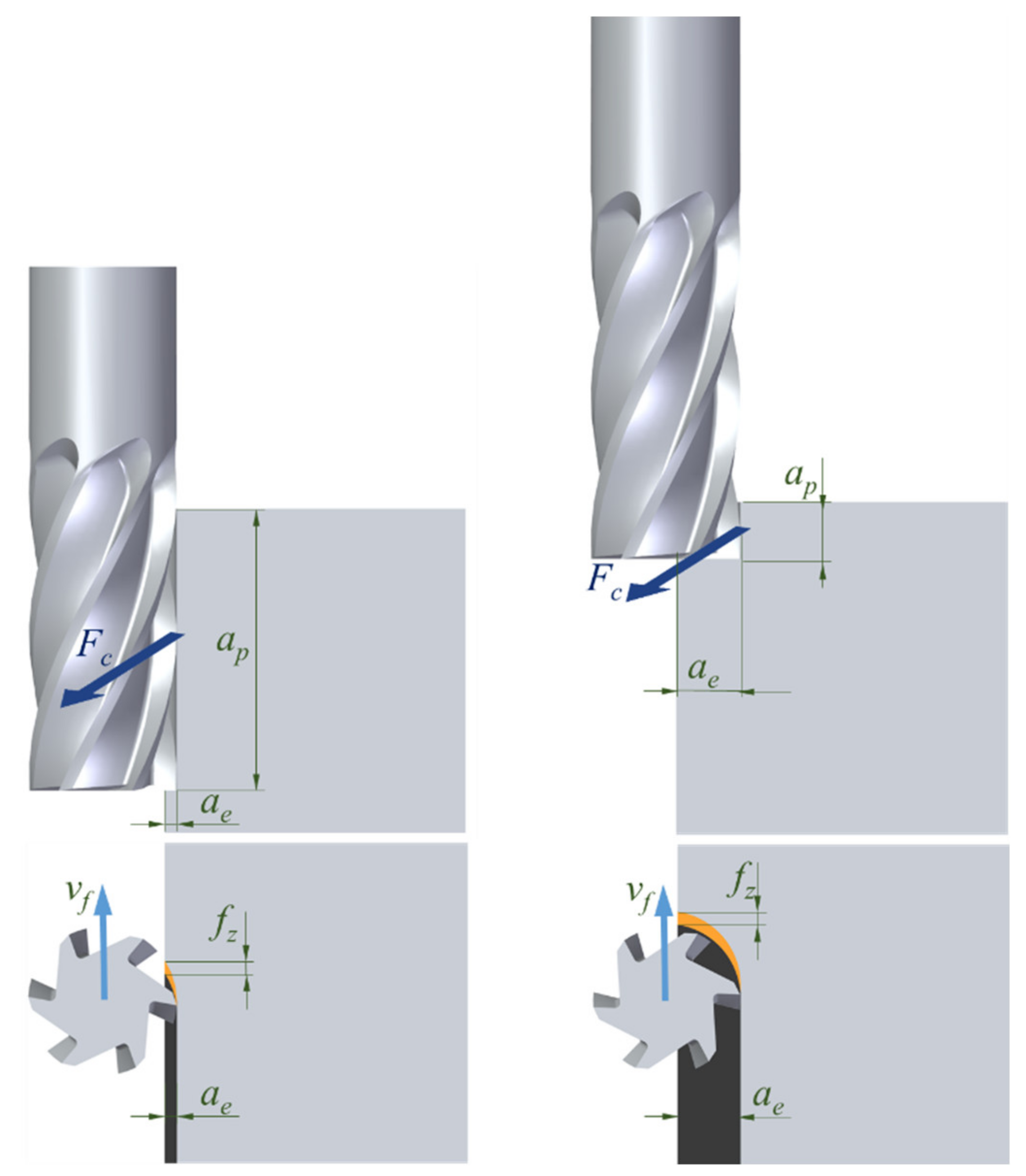
  • The tooth gap can be smaller for the same feed (the chip width is reduced), so more teeth can be implemented and, for the same feed per tooth, the final feed rises and, as a result, the machining time decreases.
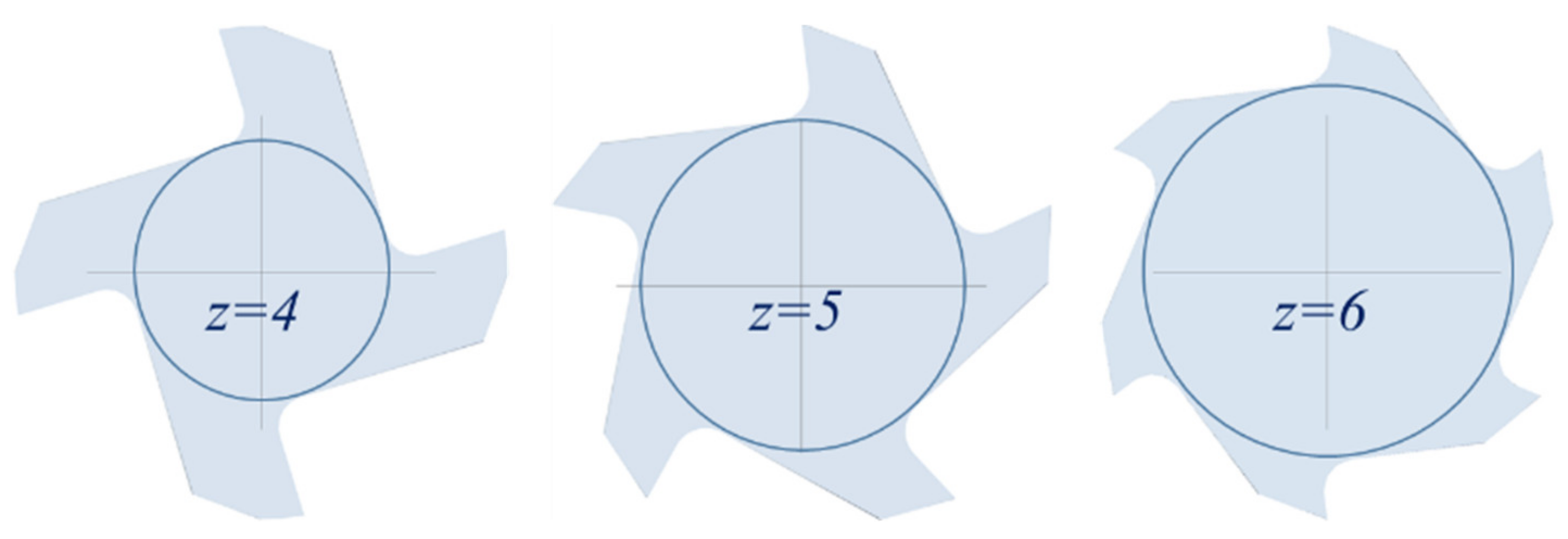
  • As a consequence, the mill core has a wider section, being able to support bigger flection and torque forces, Figure 3. This bigger rigidity makes possible to decrease deformation and vibrations, being more suitable for materials with superior cutting requirements [4], such as titanium and nickel alloys.
Figure 1 shows a straight peripheral milling, which could also follow a curved path, as in trochoidal milling, being internally generated. The chip widths are different, as shown in Figure 4 and Figure 5. There are three different kinds of feed per tooth, which are coincident in straight milling.
The engagement angle, θe, is an important parameter in peripheral millings. Different studies [5,6,7] have been based on determining this parameter and maintaining it constant.

2. Materials and Methods

2.1. Selection of the Radial Cut Depth

The radial cut depth was selected as a parameter for the trochoidal milling. The chip thickness, h, is a parameter that tool manufacturers use [8,9,10]. The process to obtain this parameter has been previously published in different classical books [11,12,13,14]; nevertheless, it has been mentioned below in order to clearly establish the approximations adopted in this study.
Parameters θe and h are clearly related, as shown in Figure 4, considering the maximum chip thickness and approximating the CB chord to the tangent in B. This approximation is valid because the feed per tooth, fz, is small in comparison to the mill dimensions. In this case, the feed per tooth, f’z, on the milling surface, is equal to the feed per tooth, fz, in the centre of the mill:
sin θ e = h m a x f z
cos θ e = r m a e r m
Converting the cosine in sine and replacing (2) in (1):
1 1 + a e r m 2 2 a e r m = h m a x f z
Other aspects to take into account include:
  • Considering that ae is small in comparison to the milling tool radius rm.
  • Avoiding the use of the squared parenthesis. According to the previous aspect, it is not significant compared to the other equation terms.
  • Using the milling tool diameter instead of the radius.
Finally, the previous expression (3), can be written as follows:
h m a x = 2 f z a e D
Applying the mean value theorem to Equation (1), the mean thickness can be obtained:
h m = 2 f z a e D θ e    
Which can also be written as:
  h m = f z a e D
Milling tool manufacturers give the cutting values referring to the feed per tooth fz, which is required to determine the feed:
F = f z · z · N
For the straight milling path, fz = fz′.
In trochoidal milling, the path of the milling tool is not straight, but curved. The most frequent path describes a real trochoid, although other curves can be applied to maintain the engagement angle θe as constant as possible.
It is necessary to pay attention to the curved paths, noting that the most interesting path for this purpose is the interior (concave) path, as in Figure 5, where the curvature and depth are constant. The engagement angle is:
cos θ e = r m a e f f r m
Equation (8) is similar to Equation (2), but includes the effective radial depth aeff, which has a much higher value, compared to ae. Furthermore, the feed per tooth and, therefore, the feed in (7) are different in the centre of the milling tool, which is the point to be programmed in the numeric control (NC) machine, and in the most external point (highest cut radius), as shown in Figure 5.
f z = f z r r + r m = f z r r + r m a e
Analysing Figure 4 and Figure 5, it can be observed that:
  • For the same feed in the milled part, the programmed feed must be lower in the interior tool path.
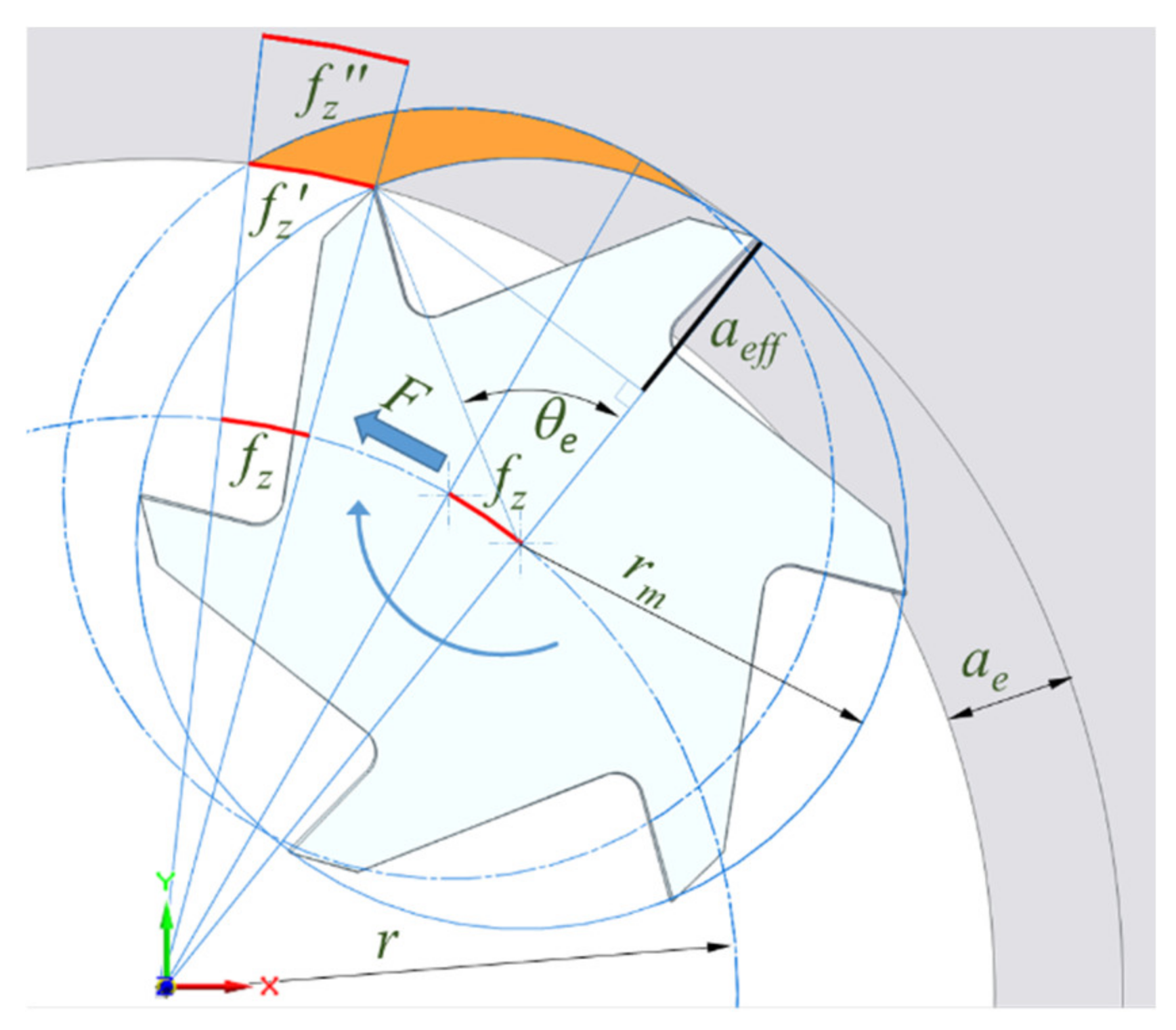
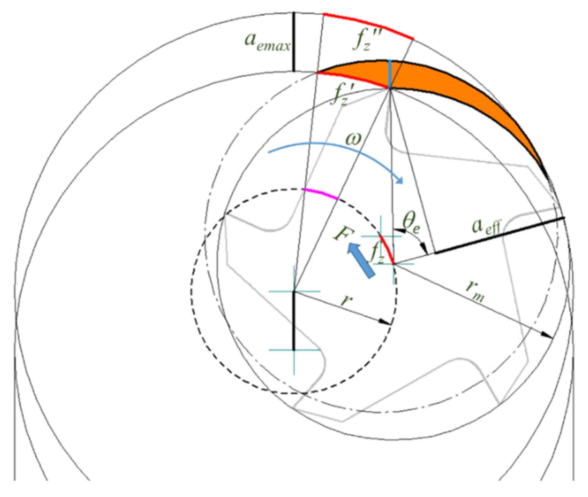
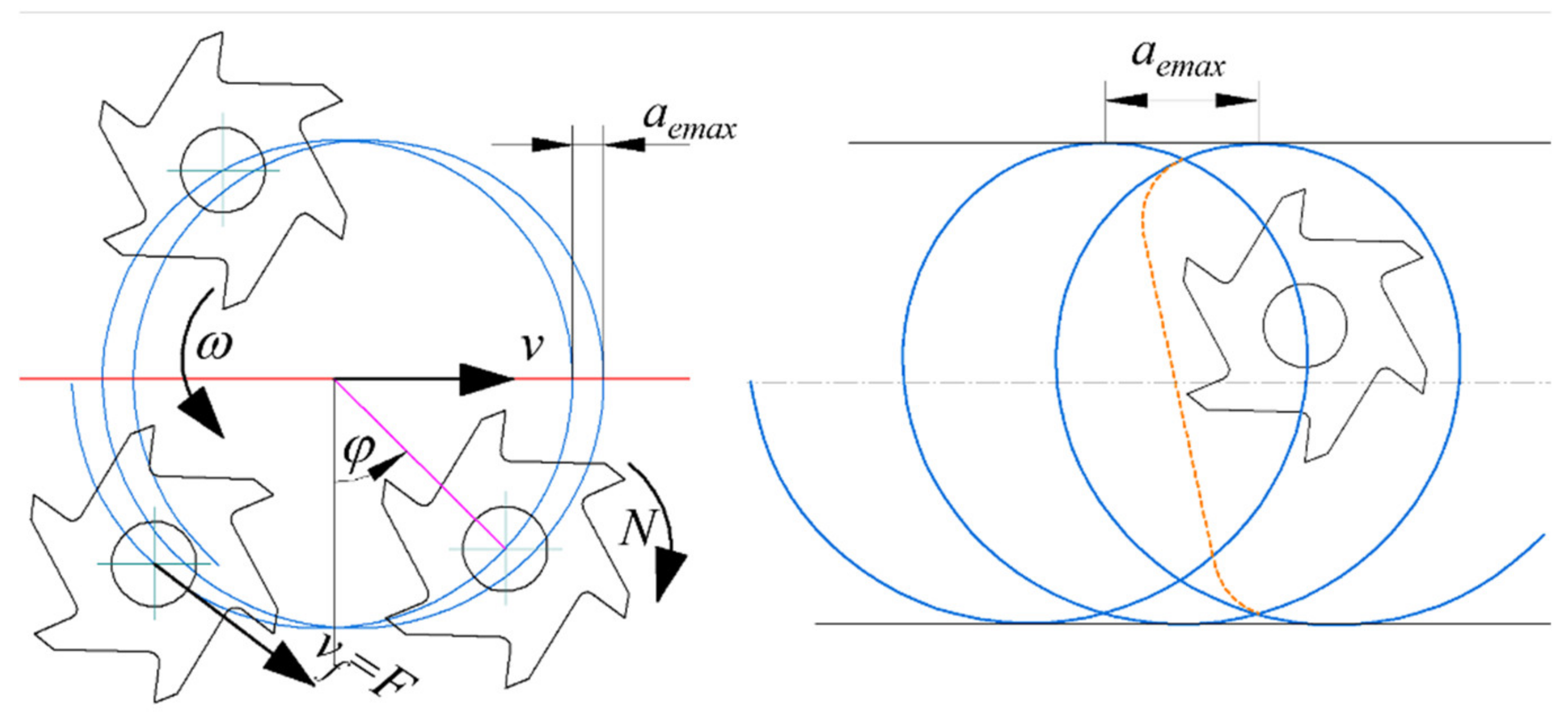
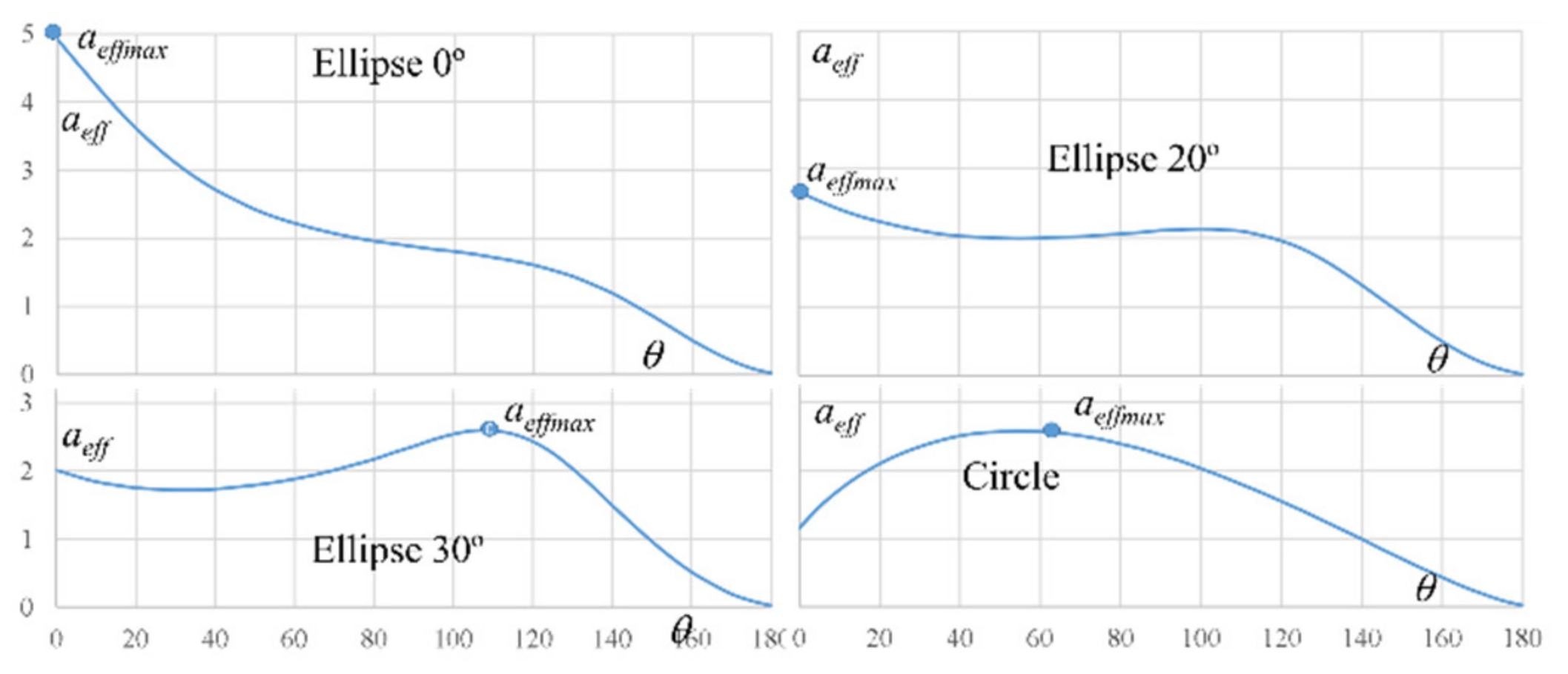
  • According to Figure 5 and Equations (2) and (8), for the interior tool path, the engagement angle is higher for the same radial depth, ae, as aeff is larger than ae.
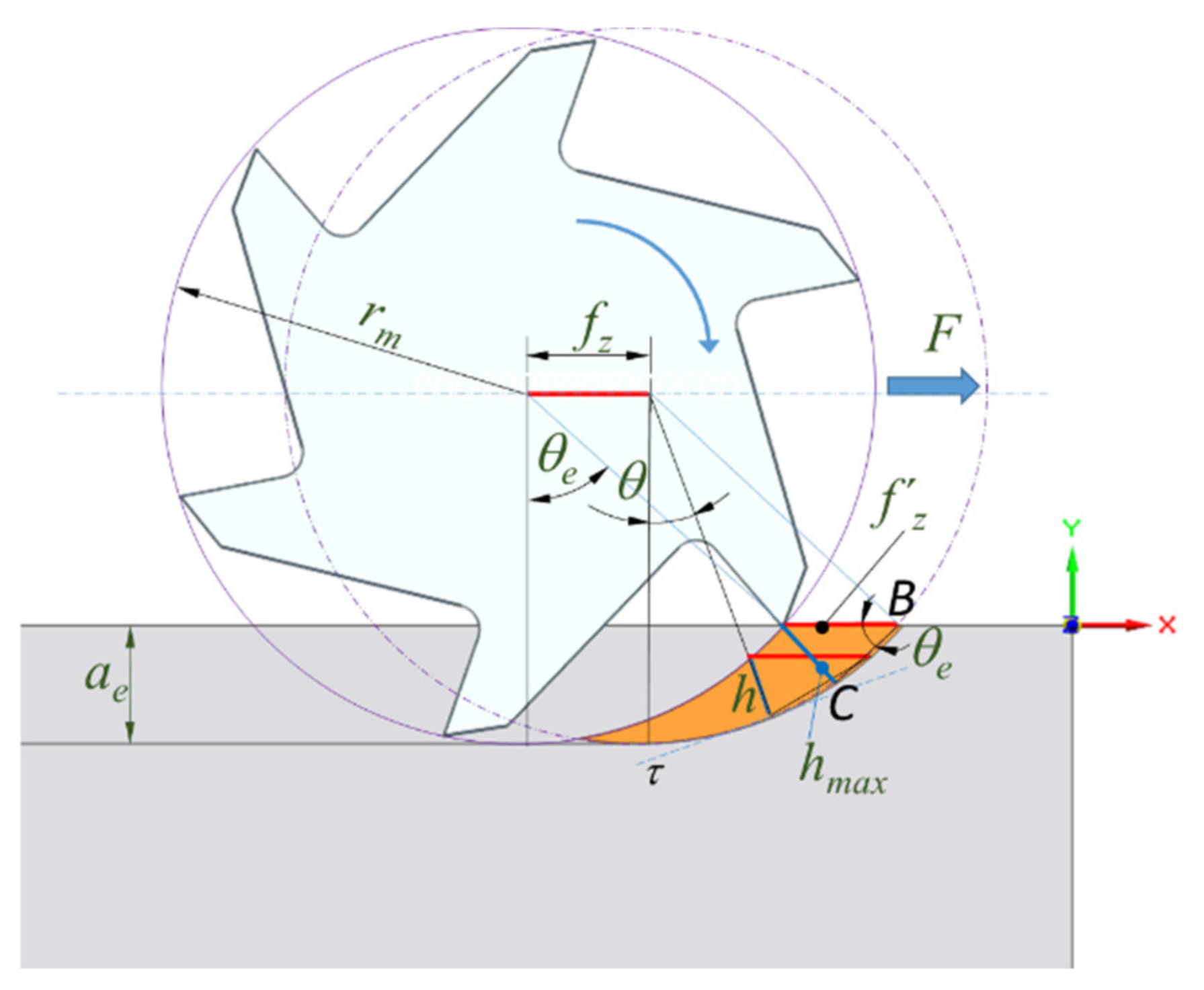
  • As the value of the feed per tooth is low in comparison to the milling tool dimensions, the arch of fz′ is close to a straight line. Thus, the mean thickness can be approximated to the previous case, considering aeff instead of ae:
      h m = f z a e f f D
  • As ae is constant, the values of the engagement angle and the effective axial depth are constant. However, they are not constant in trochoidal milling.
Moreover, the following considerations must be taken into account:
  • Avoiding an excessive decrease of the chip width, as the friction of the part with the tool edge increases, heat is generated [15]. On the contrary, the increase of the chip effective width causes a decrease of friction and cut pressure [16].
  • The mean chip depth should not be decreased. For this reason, in this study, to let hm be constant when aeff varies, the feed per tooth fz′ will be continuously modified.
In the experimental stage, fz was selected according to the tool manufacturer’s technical advice in relation to the straight-line peripheral milling for surface finishing. With that value in Equation (6), hm can be obtained. This value makes it possible to obtain fz′ in Equation (10). The instantaneous feed per tooth in the centre of the milling tool can be obtained with (9) for each instantaneous ae.
The trochoidal path is similar to the case in Figure 5, although the axial depth ae is not constant and, consequently, neither is aeff. For this reason, the engagement angle θe is variable.
Figure 6 shows a simplified approximation of the trochoidal milling path as a series of semi-circular arches with a step equal to axial depth, with values from zero to aemax.
The effective axial feed is considered the variable to be studied in the experimental stage. Its maximum value can be observed in Figure 7, when the first contact point of the milling tool is in line with the two centres (of trochoid arch and of milling tool).
The position angle γ of a point of the trochoidal path, referred to the axis of the rotation centre, will be obtained. It must be noticed that this is an approximation in which the maximum axial depth is much lower than the slot width, being as that the value of b equal to half of this slot width.
The goal is to determine the angle ωt (which is the position of the milling tool in the trochoidal path) and the maximum value of aeff.
In the triangle O2HT1, with r = b r m :
r m 2 = b a e m a x 2 + r 2 2 b a e m a x r cos β
cos β = b a e m a x 2 + r 2 r m 2 2 b a e m a x r
φ a e f f m a x = π 2 cos 1 b a e m a x 2 + r 2 r m 2 2 b a e m a x r
O 2 M = b e e m a x cos β a e f f m a x = b O 2 M
a e f f m a x = b b a e m a x 2 + r 2 r m 2 2 r
Figure 8 shows the calculation of the effective radial depth aeff. To do so, there are two possibilities: using analytic geometry or trigonometry. In both cases, the coordinate origin is placed in O2.
For the first method, solving equations with the centre in O1 and in H, T1 is obtained.
x 2 + y a e m a x 2 = b 2 x r cos ω t 2 + y r sin ω t = r m 2 x T 1 = x y T 1 = y      
Solving equations of the circles with centres in O2 and H, T2 can be obtained:
x 2 + y 2 = b 2 x r cos ω t 2 + y r sin ω t 2 = r m 2 x T 2 = x y T 2 = y      
The coordinates of M can be obtained with the equation of the straight line which contains O2 and T2, intersected with the line which contains T1 and is perpendicular to the previous one:
y = y T 2 x T 2 x y = y T 1 + x T 2 y T 2 x x T 1 x M = x y M = y
Now, the effective width MT2 can be obtained:
a e f f = x T 2 x M 2 + y T 2 y M 2
It is important to consider the double solutions of (14) and (15) in the change of quadrant, as well as the divisions by zero in (16).
The second method is based on the application of trigonometry:
O 1 T 1 = O 2 T 2 = b
x 2 = b cos ω t           y 2 = b sin ω t
O 2 H = O 2 T 2 H T 2 = r = b r m
x H = b r m cos ω t         y H = b r m sin ω t
O 1 H = x H 2 + y H + a e m a x 2
In the triangle O1HT1, the cosine theorem is applied:
r m 2 = b 2 + O 1 H 2 2 b · O 1 H · cos β
cos β = b 2 + O 1 H 2 r m 2 2 b · O 1 H
cos γ = x H O 1 H
The coordinates of point T1 are determined as follows:
x 1 = b · cos γ + β y 1 = b · sin γ + β a e m a x
The side T1T2 of the triangle T1HT2:
T 1 T 2 = x 2 x 1 2 + y 2 y 1 2
The engagement angle is obtained with the cosine theorem in the isosceles triangle T1HT2:
T 1 T 2 2 = r m 2 + r m 2 2 r m · r m · cos θ e
cos θ e = 1 T 1 T 2 2 2 r m 2
With this, the segment HM is:
H M = r m cos θ e
And the effective radial depth can be obtained:
a e f f = H T 2 H g M = r m 1 cos θ e
A different method, based in parametric CAD, was applied with Solid Edge™, as shown in Figure 9, with the values of the angle ωt from a table of variables and a spreadsheet. This method was important to verify the results of the two previous calculations.
In the NC program, the feed was variable in order to maintain constant the value of the chip width, improving the process efficiency [17]. This variation in the feed F is possible thanks to the kinematics of the milling machines and the NC, which can process large numbers of program lines [18], such as the was used in this case.
Finally, the trigonometry-based method was chosen to simplify implementation in the NC programming. This option made it possible to avoid divisions by zero or considering double solutions, as previously detailed.

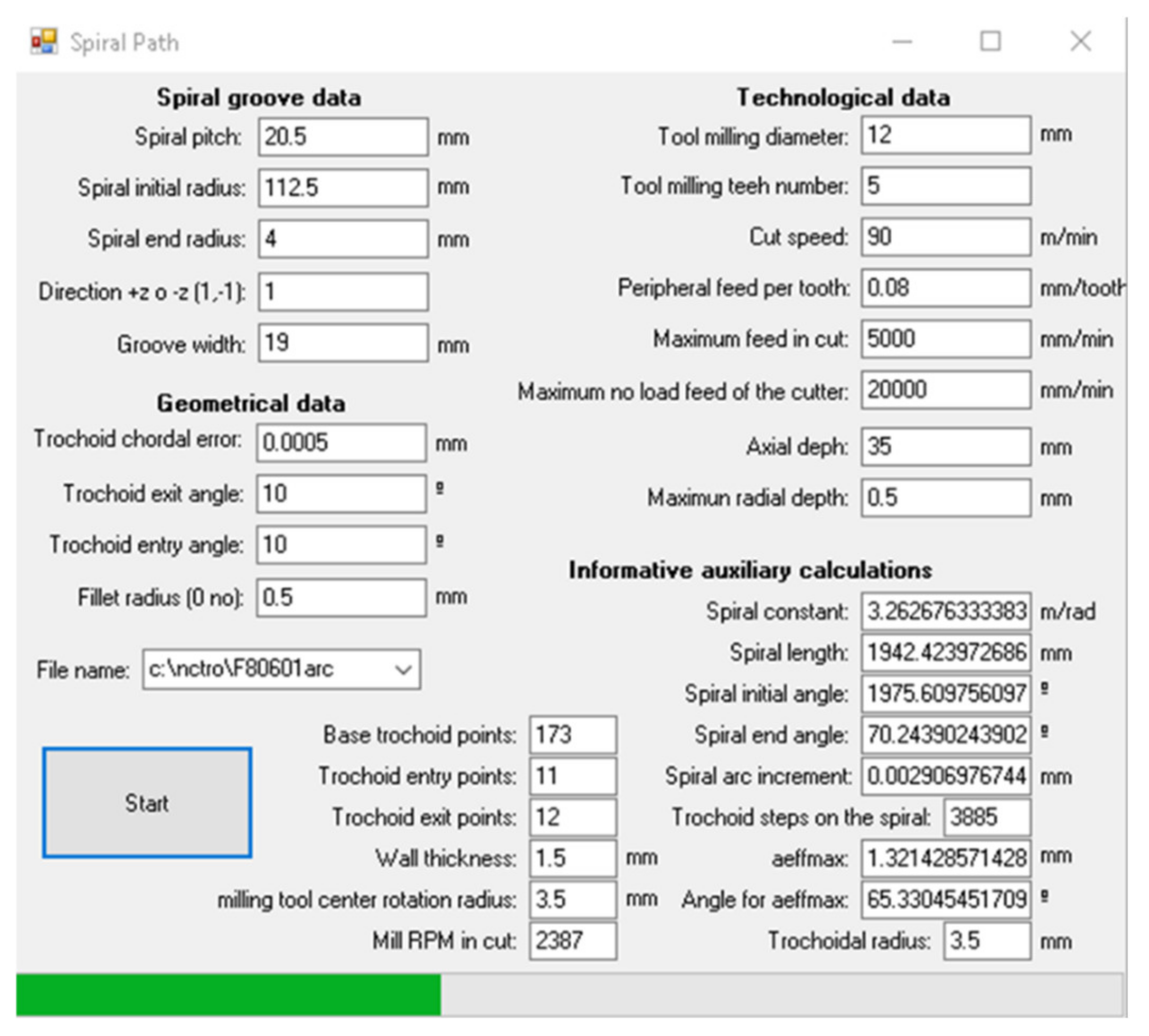
2.2. NC Program of a Trochoid with Adaptive Feed

The trochoidal path [19] described by the centre of the milling tool is the combination of two simultaneous movements. Figure 10 shows a circular path with radius r and a straight movement with a speed v.
The movement of the milling tool centre is a straight line, but this carrier route can be any 2D or 3D curve. Finally, the straight-line path will be transformed into an Archimedes spiral.
To decrease the processing time, the in and out paths are usually modified to shorten the milled area with a straight line (with initial and final tangential arches) at a higher feed [20].
The described angle depends on the angular speed ω at which the centre of the milling tool plots the circular path which, if the value of ω is constant, is φ=ωt. This value of ω can be variable, as analysed below:
The feed of the tool should be adapted to the chip thickness for each instant. When the chip thickness is the maximum, the feed is the minimum (this is similar to a progressive entry, but without constant slope), as shown in Figure 11. In the following segment of the turn, the feed of the milling tool is at the minimum at the beginning and progressively increases until reaching its maximum value as a function of the effective depth.
The previous variation is not lineal. The maximum value of the effective radial depth is in Equation (12). Its variation depends on Equation (27), following the steps between Equations (18) and (26). The graph displayed in Figure 12 was obtained with the following values: b = 0.5 mm, Dm = 12 mm, aemax = 0.5 mm. The maximum value of the effective radial depth is 1.32 mm, and the corresponding ωt angle is 65.3°.
Equations for the straight trochoidal path, with constant feed, are developed below. These equations will be the base for adapting the feed and transform the straight path into a spiral trajectory.
The angular speed ω, is obtained from the feed per tooth fz, the number of teeth z, the cutting speed Vc and the milling tool diameter Dm. The rotation frequency of the milling tool is:
N = 1000 V c π D
The feed of the cutter on the path:
v f = f z · z · N
This feed is also the tangential speed of the tool centre path, so:
v f = ω · r ω = v f r = f z · z · N r
Units can be found in the initial variable table.
The rotated angle is:
φ = ω · t
For the time, T, required for the tool centre to describe a complete rotation (φ = 2π), the simultaneous lineal movement of the path must trace the maximum radial depth aemax.
T = a e m á x v = 2 π ω v = ω 2 π a e m á x
Replacing the ω of Equation (30) in (32):
v = f z · z · N · a e m á x 2 π · r
With all this, it is possible to obtain the trochoidal path equation, depending on the milling parameters, by combining the lineal and rotational movements:
x = v t + r cos ω t + φ 0 y = r sin ω t + φ 0
Time goes from 0 to a final value tf (Figure 12):
t f = l m v
The time increase to obtain the points (x, y) that define the tool centre path can be calculated from the maximum chordal error [21]. The objective is to replace arches by segments by means of the G1 command for lineal interpolation, as well as by the activation of the high-speed functions in the NC.
When the arch of the trochoid, traced by the tool edge, is approximated to a circumference arch (Figure 13):
Δ φ = 2 cos 1 1 e r + r m
Obtaining:
Δ t = Δ φ ω                           0 < t < t f
The obtained points will be used to establish the feed in every segment. Thus, Equations (29)–(35) depend on mean feed, although for each time increment (37) there is a specific feed value, vf, which provides a different v for each φ.
Previous equations were programmed using MS Excel™ and Visual Studio™, obtaining higher processing speeds with the latter. The cutting parameters were established according to the technical advice in two manufacturer’s websites: Sandvik™ [22] and Seco™ [23]. The depth value was increased up to 35 mm for a 12 mm milling tool, with an effective cutting length of 36 mm, according to the indications of the local manufacturer (Marena, S.L., Zaragoza, Spain). This made it possible to test the performance of the milling tool in a 19 mm wide groove (so the radius of the trochoidal arch is 3.5 mm).
Instead of the total straight path, a single period is traced in order to use, for each interval between points, a different feed (10) with an effective thickness (27).
Equation (37) was not considered due to the variable values of feed, because the angular movement was not constant. The process was:
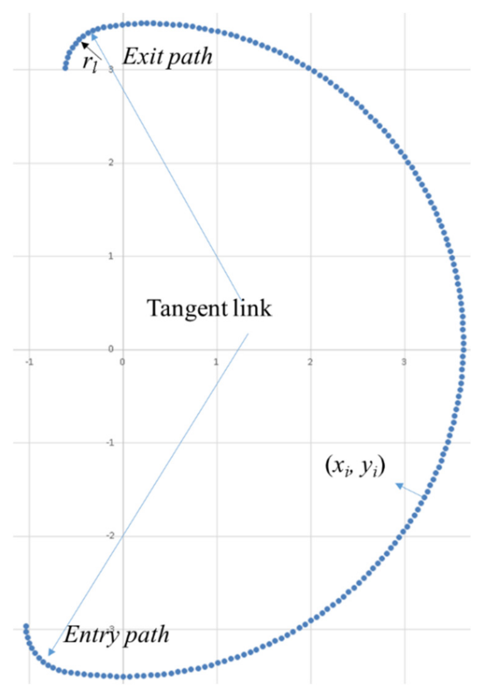
  • The points that define a step of the trochoidal path were obtained using (36).
  • ω was obtained from (30), using the feed fz for peripheral milling.
  • Introducing the previous values of Δφ and ω in (37), Δt is obtained.
  • With (33), v is obtained.
  • Using (34), the coordinates of the trochoidal arc (0 to π) were obtained, with Δφ.
  • For each of the previous coordinates (x, y), the effective chip width was obtained (27).
  • The mean value of chip width was obtained from (6), for the peripheral milling, with ae = aemax.
  • With (10), the value of fz can be found.
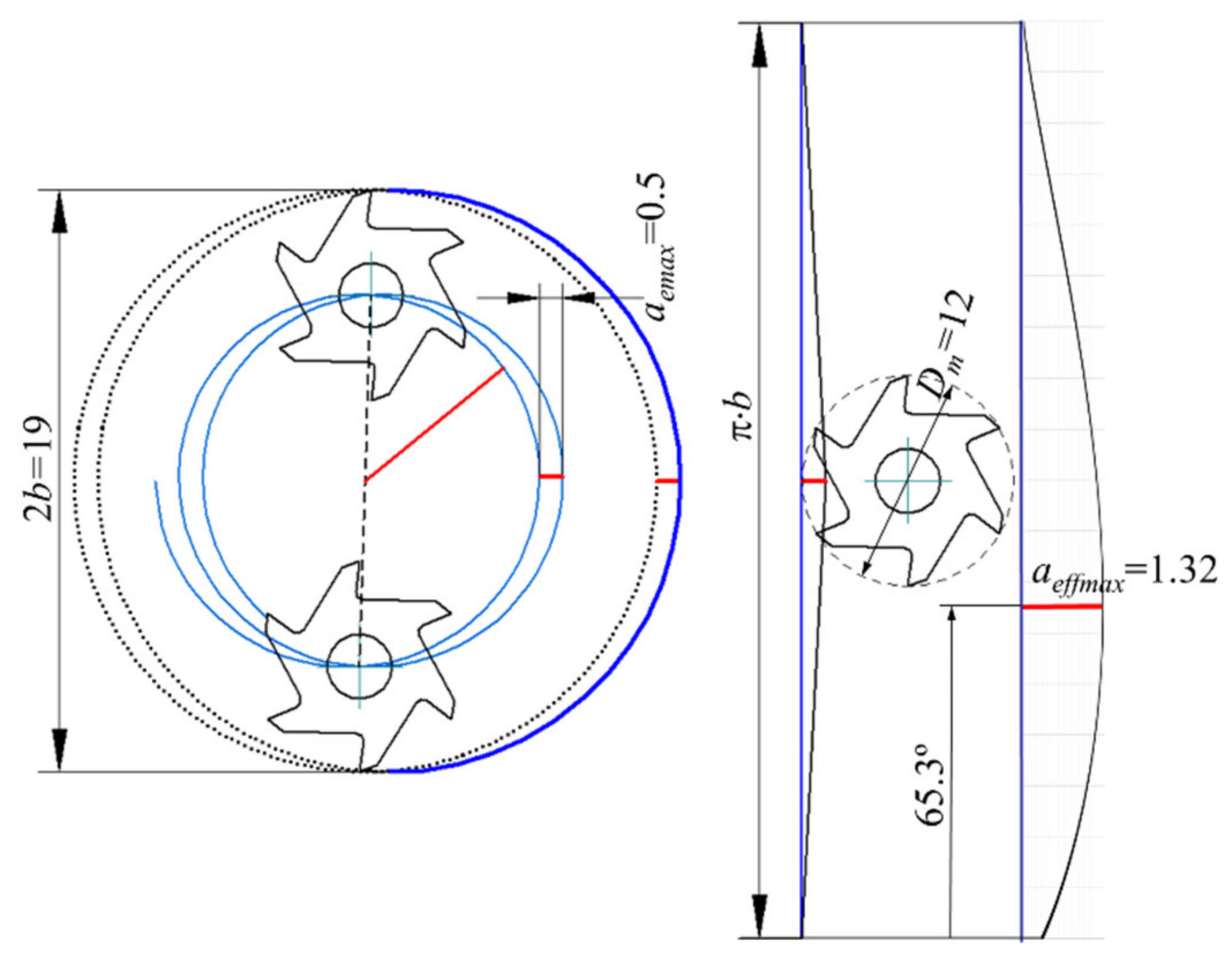
  • As the cut is interior, Equation (11) makes it possible to find the corrected fz for each point. When aeffmax is reached, fz is at the minimum, being maximum in the trochoid limits (Figure 11).
  • Finally, rotation (38) and translation are applied to the points obtained in the previous step. This step is described below.
The two reasons to mill a spiral groove (Figure 14) are:
  • The cost of a cylinder (∅ = 183 mm) of Ti-6Al-4V was significantly lower than a rectangular plate. In fact, the local provider had a leftover, which made it more affordable.
  • The milled part has concave and convex walls. While the values of the radius of these walls are not constant, this situation is closer to reality and can be consider a novelty compared to previous tests with trochoidal milling [24,25,26,27].
The point with coordinates (xi, yi) belongs to the arch of one of the trochoidal steps (Figure 15). A rotation is applied to this point:
x p i = x i cos τ y i sin τ y p i = x i sin τ + y i cos τ
The rotation is given by the direction τ, which is tangent to the spiral path, Figure 16. After this rotation, a translation is applied to the spiral point (xs, ys), where the tangent was obtained.
The coordinates of the point S (xs, ys) are:
x s = k ϕ s cos ϕ s y s = k ϕ s sin ϕ s
The direction of the spiral tangent is obtained from:
d x s = cos ϕ s ϕ s sin ϕ s d y s = sin ϕ s + ϕ s cos ϕ s
To obtain the direction of rotation, τ, the arc tangent of dy/dx must be calculated. It must be considered that a division by zero can be solved as follows:
Select Case dx
Case 0
If dy > 0 Then τ = Pi/2 + Pi Else τ = -Pi/2 + Pi
Case Else
τ = Math.Atan2(dy, dx) + Pi
End Select
It can be noticed that π has been added in the previous code, so when the spiral path is from the outside to the inside, the tangent direction is contrary to the one in Figure 16.
The Visual Net function ATAN2 made it possible to obtain the arc tangent and to distinguish the sign properly.
The entry and exit paths shown in Figure 15 are circular arches, where a value of the minimum radius depends on the acceleration performance of the machine [28], given by:
a n = v f r l 2 = f z · z · N r l 2
In order to avoid additional calculations, the entry and exit paths can be extended, as shown in Figure 17, following the same trochoidal path. From the exit, the maximum feed can be used (G0 can be too fast for some milling machines). In the entry point, the required feed is recovered.
The essential points of the trochoidal path in Figure 15, in addition to those additional ones for the entry and exit, are previously calculated, storing their coordinates and feed (x, y, F) in numeric arrays. The entry and exit points are also stored with the assigned feed.
The next step would be distributing the points of the trochoid step along the spiral. Dividing the spiral length [29] by the step (aemax) gives the number of the generated trochoidal arches. Several expressions can be used to define the length of the spiral arch. Applying differential calculus:
Δ l m = 1 2 k ϕ 1 + ϕ 2 + ln ϕ + 1 + ϕ 2 ϕ i ϕ e
When the spiral step decreases, an approximated expression of this length can be deduced:
r s = k ϕ
Using the mean value of the radius:
r m = r i + r e 2 = k ϕ i + ϕ e 2
Multiplying the mean radius by the covered arch, the arch length can be obtained, approximating with:
Δ l m = k 2 ϕ e 2 ϕ i 2
The number of trochoidal arches is:
n s p = Δ l m a e m a x
This solution was applied to the integer value plus one, because a verification of the accumulated length would make possible to stop calculations, not exceeding the value of Δlm, obtained with (43).
From Equation (36), for a given value of the chordal error, the angle increment can be obtained. As the angle traced by the trochoid is π radians, the number of points (without entry and exit points) included in Figure 15 are:
n t = truncate π Δ φ + 1
In an open path, the number of the defined points is equal to the gaps plus one.
The entry and exit points are added to the previous ones (48), as shown in Figure 17.
n i = truncate φ i Δ φ + 1 n o = truncate φ o Δ φ + 1

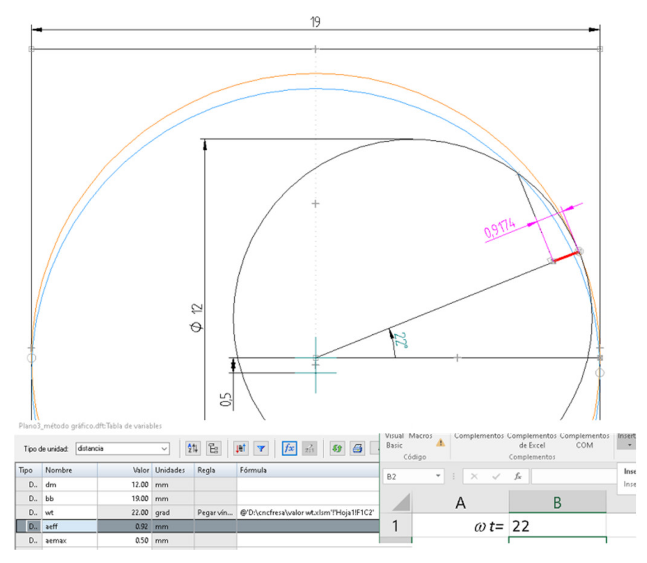
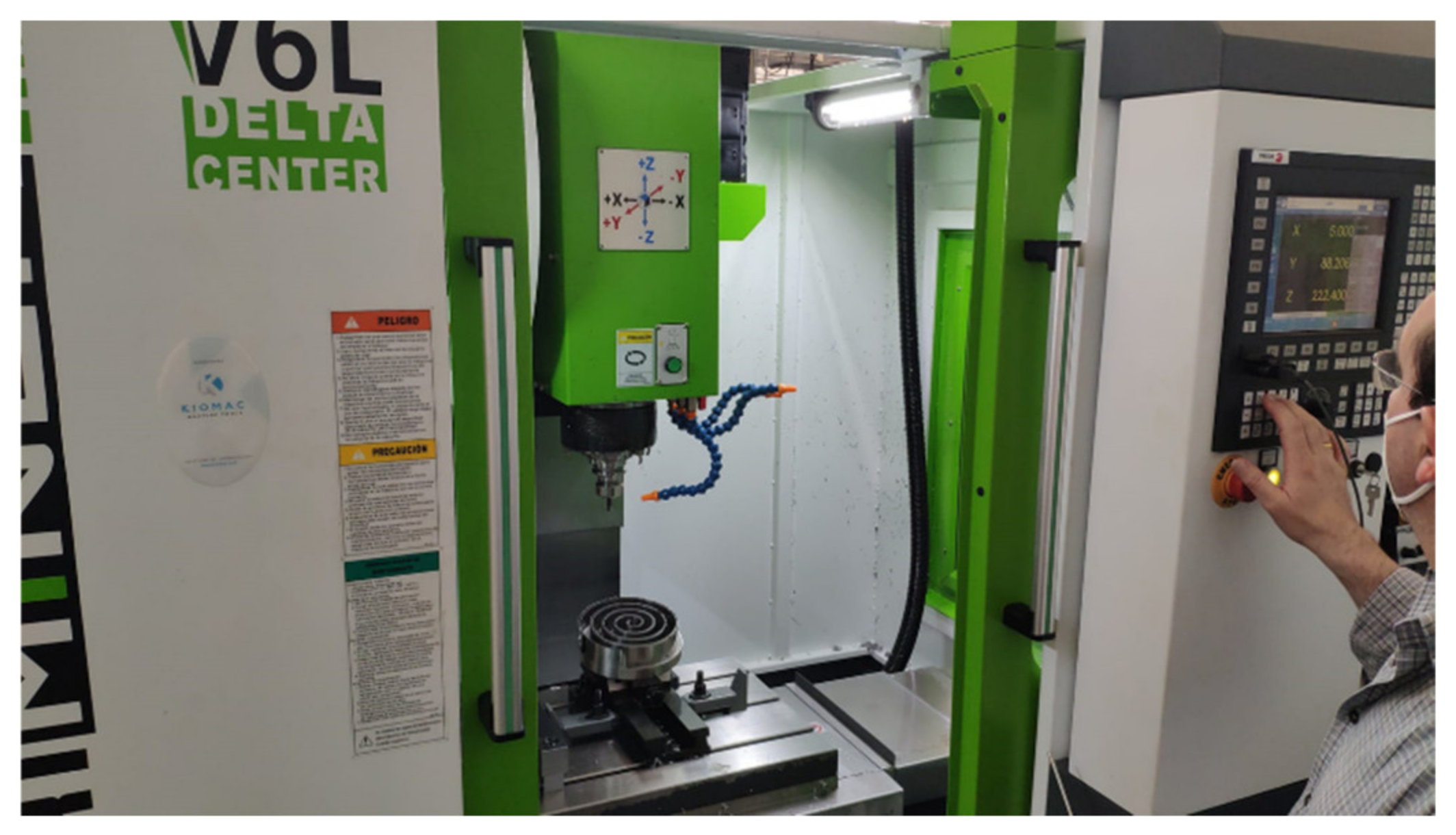
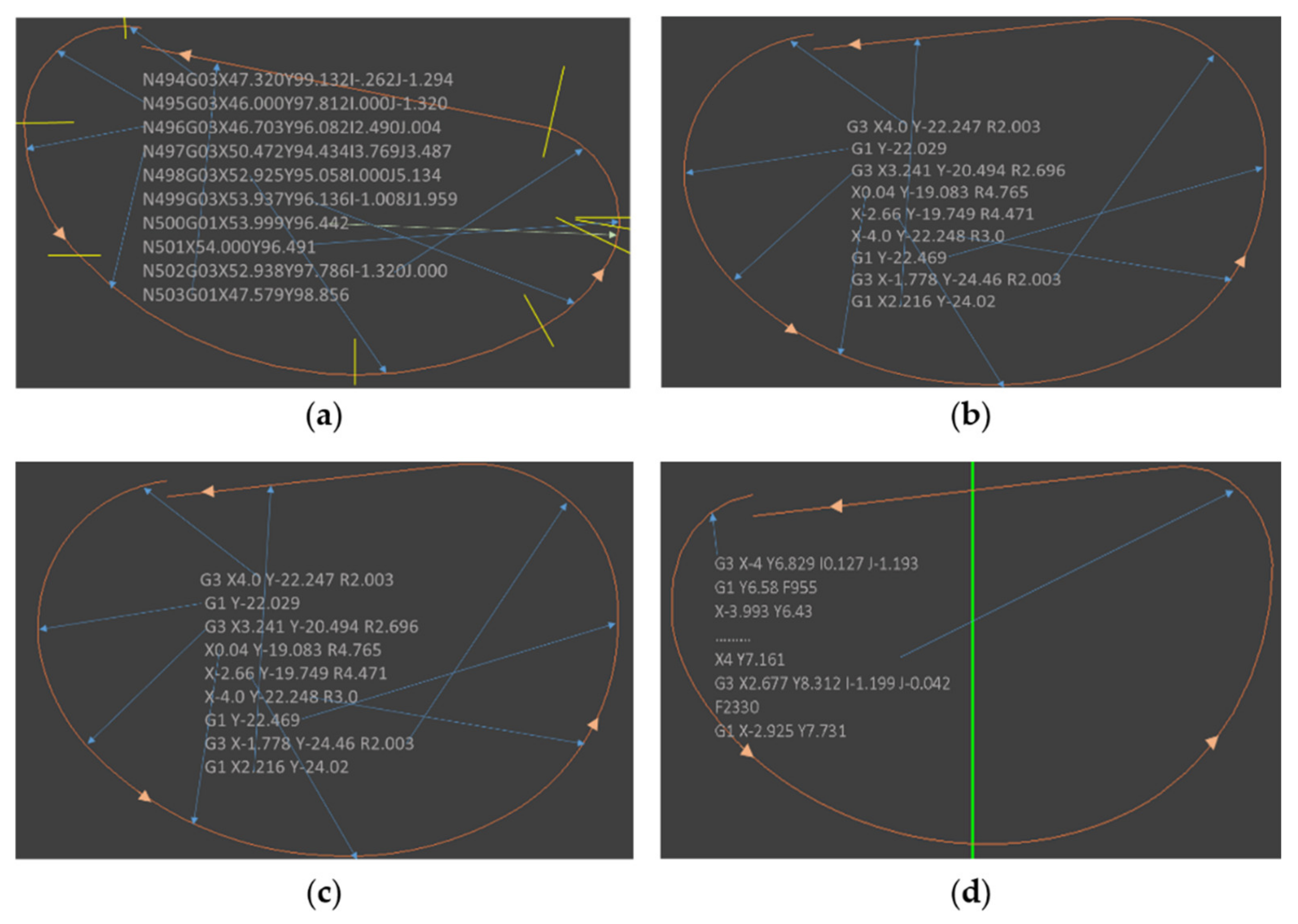
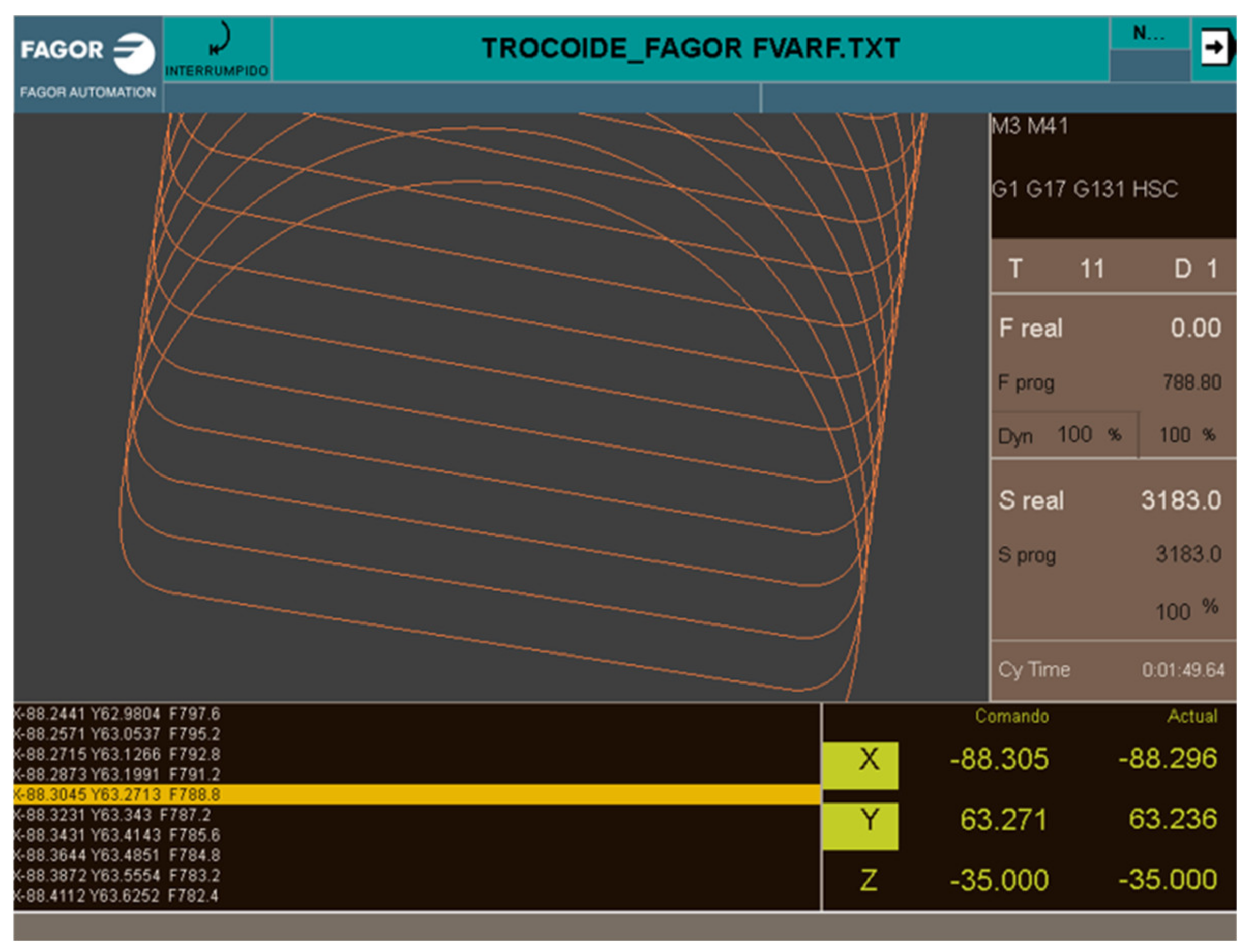
2.3. Practical Development

The trochoidal milling test was developed with a cylinder of titanium grade 5 with the previously mentioned dimensions. The initial cylinder was cut in three parts, with an appropriate saw, to develop the experimental stage using milling machines with the same features in three different vocational training centres, from Zaragoza, Valls and Puertollano (Spain), Figure 18.
The dimensions of the spiral groove and the working conditions for the peripheral milling were placed in a Visual Net form, Figure 19.
Intermediate calculations were obtained from Equation (46), making it possible to solve the final angle without any numerical approximation from the arch length and the initial angle. With this equation, a small error is generated.
For each point of the trochoidal path arch (Figure 16 and Figure 18), the rotation of Equation (38) was obtained with:
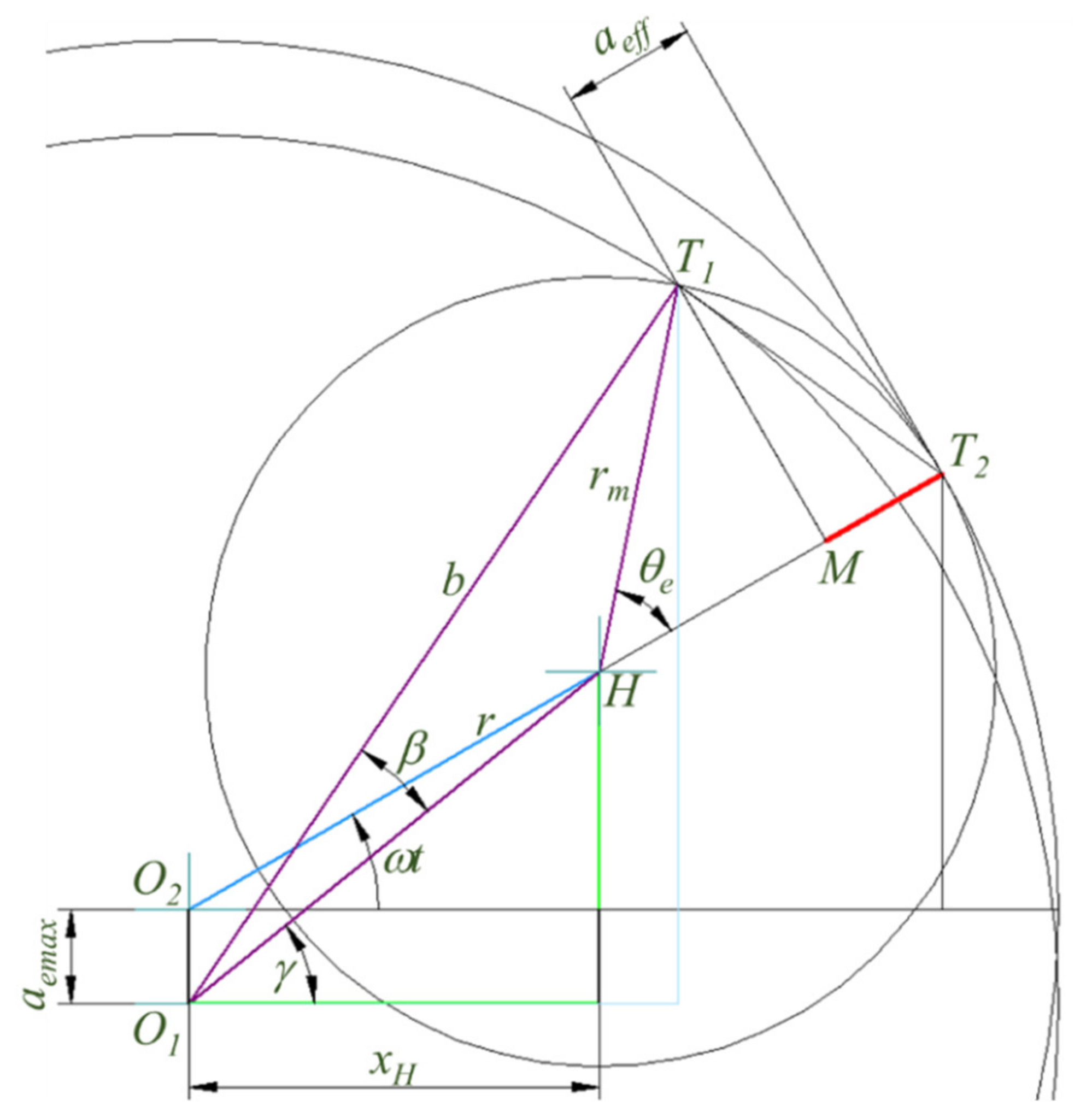
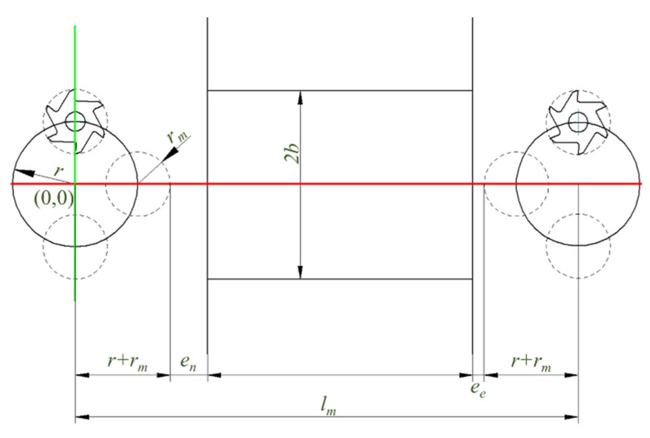
  • The substitution of angle φe (46).
  • The substitution of the length increment Δlm by the value of aemax divided by the value obtained from (48).
The angle previously obtained is introduced again in (46), repeating the process until the spiral final angle.

3. Results

Before the milling stage, two different CAM dealers were asked for the roughing of a straight groove with the dimensions shown in Figure 19 and a length of 100 mm, applying trochoidal paths (Figure 20a,b). It was also developed by us, using two additional CAM (Figure 21). From these results, a complete trochoidal arch was isolated. The only restriction was to apply the Y axis as the milling direction.
These CAM codes make possible to identify when the milling tool is not cutting (highest feed) and it is cutting (recommended feed, which remains constant).
The geometry is similar with all the CAM codes, although they describe an elliptical trochoidal path, being the semi-axes of (b) and (d) oriented in the opposite direction to (a) and (c). The intention is to replace the position and the value of aeffmax and to decrease the value or φaeffmax.
(a) and (b) are based on circular arches, while (c) and (d) are described by a series of points, following the path.
(b) and (c) add two straight segments, in parallel to the milling direction, in order to improve the finishing.
The entry and exit paths are circular arches (G3) in all of the cases.
The slope and transformation of an elliptical trochoidal path was previously studied [30]. In this research, the elliptical trochoid was graphically analysed, as seen in Figure 9 and Figure 21.
Figure 22 shows the variation of aeff and the milling displacement angle with increments of 5°.
The 20° elliptical path keeps the value of aeff more stable, being necessary to optimize its parameters [30,31]. However, the circular trochoidal path was tested, with the objective of studying the feed per tooth variation to maintain the chip thickness constant.
Figure 23 shows the path of the milling tool centre, combining Figure 15 and Figure 16, thus extending the trochoidal arch and rounding entry and exit paths.
During the tests, the milling tool “marena 965” (Figure 24) was used [32], with z = 5 teeth, ∅ = 12 mm, maximum cutting length = 36 mm. The cutting speed was 90 m/min and the feed was 0.08 mm/tooth for peripheral milling, with ae = 0.5 mm and p = 35 mm. With these conditions, the spiral path was milled several times with three similar machines (Figure 17).
Figure 25 shows the path in the NC display (FAGOR 8060TM).
Figure 26 shows the real spiral after milling it (left), and the initial (a), intermediate (b) and final (c) Titanium chips.
Finally, Figure 27 and Figure 28 show the tool wear obtained with constant F and with variable F, respectively.

4. Discussion

As shown in Figure 22, the 20° elliptical path can be interesting because aeff stays more stable, although its value is higher, decreasing the feed per tooth. In contrast, the 0° elliptical path starts with a high value of aeff, making it necessary to decrease the feed per tooth, although it could be increased at the exit.
The circular trochoidal path was chosen because its initial aeff is not high, obtaining its maximum value before tracing the centre of the semitrochoid. The feed per tooth has a high value at the entry and decreases until aeffmax and, after it, its value increases to the exit. From the exit to the following entry, the feed value can be significantly increased.
After analysing references [30] and [31], it would be interesting to test these new paths by varying the F in further research.
The tool holders must be hydraulic, particularly when the loads are high or the feeds vary a lot during the milling process, because other kinds of tool holders (e.g.,: Weldon or clamps) were not able to maintain the position of the tool.
In both milling processes, a frontal tool tooth was broken (Figure 27 and Figure 28). The tool wear was slightly lighter with variable F and the tool coating was not peeled in any case. The diameter deviation between teeth, before and after the milling, was below 5 micrometres.
The milling process with variable F, even adapting S [28,32], suggests improvements which should be tested in further research.
An additional possibility would be elevating the milling tool in the exit points (helicoidally), descending in the entry points (Figure 15 and Figure 17). This possibility was not implemented, according to the tool manufacturer indications (to avoid stress in the Z spindle and the entrapment of chip residues).

5. Conclusions

The machining time with the conditions shown in Figure 19, was 1 h 17 min with constant F, and 51 min with variable F. When the cutting speed was raised to 100 m/min and the feed per tooth was 0.07 mm, the machining times were 1 h 36 min and 59 min, respectively.
The wear of the tool edge decreases with the variable F strategy.
Finally, it was concluded that the variable F strategy was advantageous, but it can only be applied with milling machines that allow high acceleration of their axes (X, Y).
It is possible to reduce the energy consumption as well as the time required, increasing tool life and improving the sustainability of machining processes, thanks to several aspects. These aspects include the improved features of current machine tools, new machining strategies and advances in tool cooling, e.g., using cryogenic products [33] with phase change. It is also possible to use cryogenic cooling to improve the effectiveness of lubrication [34,35], significantly reducing the quantity required. Another interesting option is based on adding nanoparticles [36] to reduce tool wear or by locally applying a process of laser preheating [37].

Author Contributions

Conceptualization, C.G.-H., P.U.-A., J.-L.H.-T. and P.K.; methodology, C.G.-H., J.-J.G.-B., J.-J.V.-S., P.U.-A., J.-L.H.-T. and P.K.; software, J.-L.H.-T.; validation, C.G.-H., J.-J.G.-B., J.-A.B.-P., B.C.-Á., M.-Á.A.-S., F.V.-C., R.P.-C. and J.-L.H.-T.; formal analysis, C.G.-H. and J.-L.H.-T.; investigation, C.G.-H., P.U.-A., J.-A.B.-P., B.C.-Á., M.-Á.A.-S., F.V.-C., J.-L.H.-T. and P.K.; resources, J.-J.G.-B.; data curation, C.G.-H. and J.-L.H.-T.; writing—original draft preparation, C.G.-H., J.-J.G.-B., J.-J.V.-S. and J.-L.H.-T.; writing—review and editing, C.G.-H., P.U.-A., R.P.-C., J.-L.H.-T. and P.K.; supervision, C.G.-H., J.-J.G.-B., J.-J.V.-S., P.U.-A., J.-A.B.-P., B.C.-Á., M.-Á.A.-S., F.V.-C., R.P.-C. and J.-L.H.-T.; project administration, J.-J.G.-B. and F.V.-C.; funding acquisition, J.-J.G.-B. and F.V.-C. All authors have read and agreed to the published version of the manuscript.

Funding

This research was funded by the Spanish “Secretaría de Estado de Educación y Formación Profesional” grant for applied innovation and knowledge transfer in vocational training: AFP 19/00017, 16 September 2019.

Data Availability Statement

All data generated or analysed during this study are included in this published article.

Acknowledgments

The authors want to thank the following: Pixel Sistemas, for the CAM code in Solid Edge CAM Pro; Hexagon, for the CAM code in EDGECAM; Students of the NC and CAM modules, for simulating the NC and CAM code during the remote (due to COVID-19) practical sessions; Kiomac S.L., for the technical advice; Ysamco S.L., for preparing the Ti6V4Al parts; Marena S.L., for facilitating the access to all the required milling tools and for the technical advice.

Conflicts of Interest

The authors declare no conflict of interest.

References

  1. Harvey Tools. Hem Guidebook a Machinist’s Guide to Increasing Shop Productivity with High Efficiency Milling; Harvey Performance Company, LLC: Rowley, MA, USA, 2017; Volume 9, pp. 38–40. [Google Scholar]
  2. Pérez, J.; Llorente, J.I.; Sanchez, J.A. Advanced cutting conditions for the milling of aeronautical alloys. J. Mater. Process. Technol. 2000, 100, 1–11. [Google Scholar]
  3. Okokpujie, I.P.; Okonkwo, U.C. Effects of cutting parameters on surface roughness during end milling of aluminium under minimum quantity lubrication (MQL). Int. J. Sci. Res. 2015, 4, 2937–2942. [Google Scholar]
  4. Available online: https://www.harveyperformance.com/in-the-loupe/flute-count-matters/ (accessed on 7 May 2021).
  5. Jacso, A.; Matyasi, G.; Szalay, T. The fast constant engagement offsetting method for generating milling tool paths. Int. J. Adv. Manuf. Technol. 2019, 103, 4293–4305. [Google Scholar] [CrossRef] [Green Version]
  6. Choy, H.S.; Chan, K.W. A corner-looping based tool path for pocket milling. Comput. Aided Des. 2003, 35, 155–166. [Google Scholar] [CrossRef]
  7. Wu, S.; Zhao, Z.; Wang, C.Y.; Xie, Y.; Ma, W. Optimization of toolpath with circular cycle transition for sharp corners in pocket milling. Int. J. Adv. Manuf. Technol. 2016, 86, 2861–2871. [Google Scholar] [CrossRef]
  8. Masters in Solid Carbide Tooling. SCT Special Carbide Tooling. 2020, pp. 144–145. Available online: https://sct-tools.com/wp-content/uploads/2020/06/Catalog_2020_Downloads_SCT_Tools_.pdf (accessed on 7 May 2021).
  9. 2017 Master Cataloge. WIDIA. pp. 1266–1272. Available online: https://s7d2.scene7.com/skins/Kennametal/A-15-04580_Master17_Catalog_Metric_LRpdf (accessed on 7 May 2021).
  10. Trochoidal Shank End Mill with Variable Helix. S. v. Bassewitz GmbH & Co. KG (pp. 4 y 7). Available online: https://www.bassewitz.com/en/ (accessed on 7 May 2021).
  11. Solar, Z.C. Problemas de Tecnología de la Fresadora. Biblioteca Tecnológica de la Fabricación Mecánica; Biblioteca Tecnológica de la Fabricación Mecánica: Gijón, Spain, 1970; p. 49. [Google Scholar]
  12. Boothroyd, G. Fundamentos del corte de los metales y de las máquinas herramientas/. Geoffrey Boothroyd. Mcgraw Hill. Lat. SA. 1975, Book, 29–37. [Google Scholar]
  13. Micheletti, G.F.; Doménech, T.L. Mecanizado por arranque de viruta: Tecnología mecánica. Blume 1980, Book, 150–153. [Google Scholar]
  14. Peláez Vara, J. La Fresadora. Colección La Máquina Herramienta (TOMO II); Ediciones CEDEL: Barcelona, Spain, 1992; pp. 43–44. [Google Scholar]
  15. Richardson, D.J.; Keavey, M.A.; Dailami, F. Modelling of cutting induced workpiece temperatures for dry milling. Int. J. Mach. Tools Manuf. 2006, 46, 1139–1145. [Google Scholar] [CrossRef]
  16. Rao, B.; Shin, Y.C. Analysis on high-speed face-milling of 7075-T6 aluminum using carbide and diamond cutters. Int. J. Mach. Tools Manuf. 2001, 41, 1763–1781. [Google Scholar] [CrossRef]
  17. Perez, H.; Rios, J.; Diez, E.; Vizan, A. Increase of material removal rate in peripheral milling by varying feed rate. J. Mater. Process. Technol. 2008, 201, 486–490. [Google Scholar] [CrossRef]
  18. Fagor Automation. Manual de Programación CNC 8060 8065. Available online: https://www.fagorautomation.com (accessed on 14 May 2021).
  19. Otkur, M.; Lazoglu, I. Trochoidal milling. Int. J. Mach. Tools Manuf. 2007, 47, 1324–1332. [Google Scholar] [CrossRef]
  20. Pleta, A.; Mears, L. Cutting force investigation of trochoidal milling in nickel-based superalloy. Procedia Manuf. 2016, 5, 1348–1356. [Google Scholar] [CrossRef] [Green Version]
  21. Talón, J.L.H.; Boria, D.R.; Muro, L.B.; Gómez, C.L.; Zurdo, J.J.M.; Calvo, F.V.; Barace, J.J.G. Functional check test for high-speed milling centres of up to five axes. Int. J. Adv. Manuf. Technol. 2011, 55, 39–51. [Google Scholar] [CrossRef]
  22. Sanvik Coromant. Fresado (PDF Format). pp. 121–122. Available online: https://www.sandvik.coromant.com/es-es/knowledge/milling/milling-holes-cavities-pockets/pages/slicing-trochoidal-milling.aspx (accessed on 21 May 2021).
  23. Seco, Fresas Enterizas JABRO. (PDF Format), p. 420. Available online: https://usercontent.azureedge.net/Content/UserContent/Documents/027782.pdf (accessed on 21 May 2021).
  24. Gross, D.; Friedl, F.; Meier, T.; Hanenkamp, N. Comparison of linear and trochoidal milling for wear and vibration reduced machining. Procedia CIRP 2020, 90, 563–567. [Google Scholar] [CrossRef]
  25. Karkalos, N.E.; Karmiris-Obratański, P.; Kurpiel, S.; Zagórski, K.; Markopoulos, A.P. Investigation on the Surface Quality Obtained during Trochoidal Milling of 6082 Aluminum Alloy. Machines 2021, 9, 75. [Google Scholar] [CrossRef]
  26. Waszczuk, K.; Skowronek, H.; Karolczak, P.; Kowalski, M.; Kołodziej, M. Influence of the Trochoidal Tool Path on Quality Surface of Groove Walls. Adv. Sci. Technology. Res. J. 2019, 13, 38–42. [Google Scholar] [CrossRef]
  27. Santhakumar, J.; Iqbal, U.M. Role of trochoidal machining process parameter and chip morphology studies during end milling of AISI D3 steel. J. Intell. Manuf. 2021, 32, 649–665. [Google Scholar] [CrossRef]
  28. Garde-Barace, J.J.; Huertas-Talón, J.L.; Valdivia-Calvo FBueno-Pérez, J.A.; Cano-Álvarez, B.; Álcazar-Sánchez, M.A.; Ponz-Cuenca, R.; Tzotzis, A. Velocidad de corte constante en fresado. IMHE Ed. Técnicas IZARO 2021, 476, 80–98. [Google Scholar]
  29. Aguirre, N. La espiral de Arquímedes en un proyecto de modelación matemática. Rev. Educ. Matemática 2008, 23, 1–10. [Google Scholar]
  30. Huang, X.; Wu, S.; Liang, L.; Li, X.; Huang, N. Efficient trochoidal milling based on medial axis transformation and inscribed ellipse. Int. J. Adv. Manuf. Technol. 2020, 111, 1069–1076. [Google Scholar] [CrossRef]
  31. Klocke, F.; Bergs, T.; Busch, M.; Rohde, L.; Witty, M.; Cabral, G.F. Integrated approach for a knowledge-based process layout for simultaneous 5-axis milling of advanced materials. Adv. Tribol. 2011, 2011, 1–7. [Google Scholar] [CrossRef] [Green Version]
  32. Käsemodel, R.B.; de Souza, A.F.; Voigt, R.; Basso, I.; Rodrigues, A.R. CAD/CAM interfaced algorithm reduces cutting force, roughness, and machining time in free-form milling. Int. J. Adv. Manuf. Technol. 2020, 107, 1883–1900. [Google Scholar] [CrossRef]
  33. Huertas, J.L.; Faci, E.; Ros, E. CO2, la mejor opción. IMHE 2006, 330, 59–78. [Google Scholar]
  34. Jamil, M.; Zhao, W.; He, N.; Gupta, M.K.; Sarikaya, M.; Khan, A.M.; Sanjay, M.R.; Siengchin, S.; Pimenov, D.Y. Sustainable milling of Ti–6Al–4V: A trade-off between energy efficiency, carbon emissions and machining characteristics under MQL and cryogenic environment. J. Clean. Prod. 2021, 281, 1–14. [Google Scholar] [CrossRef]
  35. Albertelli, P.; Mussi, V.; Strano, M.; Monno, M. Experimental investigation of the effects of cryogenic cooling on tool life in Ti6Al4V milling. Int. Adv. Manuf. Technol. 2021. Available online: https://link.springer.com/article/10.1007%2Fs00170-021-07161-9#citeas (accessed on 21 May 2021).
  36. Eltaggaz, A.; Nouzil, I.; Deiab, I. Machining Ti-6Al-4V Alloy Using Nano-Cutting Fluids: Investigation and Analysis. J. Manuf. Mater. Process 2021, 5, 42. [Google Scholar]
  37. Kim, D.-H.; Lee, C.-M. Experimental Investigation on Machinability of Titanium Alloy by Laser-Assisted End Milling. Metals 2021, 11, 1552. [Google Scholar] [CrossRef]
Figure 1. Relation between ap and ae for the same section.
Mathematics 09 02701 g001
Figure 2. Micro-rounded mill cutting edge.
Mathematics 09 02701 g002
Figure 3. For the same tool diameter, with more teeth, there is a tool core increase.
Mathematics 09 02701 g003
Figure 4. Engagement angle and chip thickness in lineal path.
Mathematics 09 02701 g004
Figure 5. Engagement angle and chip depth in the interior arch.
Mathematics 09 02701 g005
Figure 6. Trochoidal path approximation.
Mathematics 09 02701 g006
Figure 7. Instant in which aeffmax is reached.
Mathematics 09 02701 g007
Figure 8. Obtaining the effective radial depth.
Mathematics 09 02701 g008
Figure 9. Graphical method to verify aeff.
Mathematics 09 02701 g009
Figure 10. Generation of the straight-line path.
Mathematics 09 02701 g010
Figure 11. Equivalence between trochoidal and peripheral ramp milling with variable slope.
Mathematics 09 02701 g011
Figure 12. Milling time calculation.
Mathematics 09 02701 g012
Figure 13. Polygonal approximation of the circumference.
Mathematics 09 02701 g013
Figure 14. Spiral groove.
Mathematics 09 02701 g014
Figure 15. Trochoidal path step.
Mathematics 09 02701 g015
Figure 16. Rotation and translation for adapting the point (xi, yi) to the spiral path.
Mathematics 09 02701 g016
Figure 17. Extension of the entry and exit paths.
Mathematics 09 02701 g017
Figure 18. One of the three NC milling machines.
Mathematics 09 02701 g018
Figure 19. Visual Net data form.
Mathematics 09 02701 g019
Figure 20. Four CAM trajectories applied.
Mathematics 09 02701 g020
Figure 21. Graphical analysis obtaining of aeff in an elliptical trochoidal path.
Mathematics 09 02701 g021
Figure 22. aeff for the circular and elliptical trochoidal paths.
Mathematics 09 02701 g022
Figure 23. Trochoidal roughing adapted to a spiral groove.
Mathematics 09 02701 g023
Figure 24. Milling tool used in the experiments.
Mathematics 09 02701 g024
Figure 25. Trochoidal-spiral path.
Mathematics 09 02701 g025
Figure 26. One of the milling processes and types of chips (ac).
Mathematics 09 02701 g026
Figure 27. Tool wear for constant F.
Mathematics 09 02701 g027
Figure 28. Tool wear for variable F.
Mathematics 09 02701 g028
Publisher’s Note: MDPI stays neutral with regard to jurisdictional claims in published maps and institutional affiliations.

