Stable Optical Solitons for the Higher-Order Non-Kerr NLSE via the Modified Simple Equation Method

Abstract

This paper studies the propagation of the short pulse optics model governed by the higher-order nonlinear Schrödinger equation (NLSE) with non-Kerr nonlinearity. Exact one-soliton solutions are derived for a generalized case of the NLSE with the aid of software symbolic computations. The modified Kudryashov simple equation method (MSEM) is employed for this purpose under some parametric constraints. The computational work shows the difference, effectiveness, reliability, and power of the considered scheme. This method can treat several complex higher-order NLSEs that arise in mathematical physics. Graphical illustrations of some obtained solitons are presented.

1. Introduction

The nonlinear Schrödinger-type equations (NLSEs) are essential to describe the optical soliton propagation in a variety of branches of fiber communication sciences, e.g., nonlinear optics [1,2]. Additionally, these models have successfully addressed the ultrashort pulses of the wave dynamics, which will increase the power of high-bit-rate transmission systems [3,4]. Consequently, understanding the dynamics of the soliton can lead to an extensive improvement in technology and industry. Therefore, there has been significant progress in the development of diverse schemes for treating NLSEs and nonlinear partial differential equations (NPDEs) in the general case. For approximate schemes, we cite the Adomian decomposition method [5,6], collocation method [7], homotopy perturbation method [8], homotopy analysis method [9], reduced differential transform method [10,11], q-homotopy analysis method [12], variational iteration method [13], reproducing kernel Hilbert space method [14], iterative Shehu transform method [15], and residual power series method [16,17]. While constructing an exact analytic solution is of more importance since this can provide the best understanding of the model’s nature to be processed in an efficient way, researchers have developed various powerful tools to analyze NPDEs. Furthermore, these can be utilized to estimate the boundary data that are used in numeric and semi-analytic methods. Such techniques include the Kudryashov method and its modifications [18,19,20], functional variable method [19], generalized Riccati equation mapping method [21], Jacobi elliptic function method [21,22], sine-Gordon expansion method [23], Hirota method [24], subequation method [25], soliton ansatz method [26], $G^{\prime }/G$-expansion method [27], new extended direct algebraic method [28], extended trial function method [29], new generalized exponential rational function method [30], integral dispersion equation method [31,32], modified extended tanh-function method [33], simple equation method [34,35], and modified simple equation methods [36] (see also the references that appear therein).

In the present work, we aim to analytically process the higher-order NLSE with derivative non-Kerr nonlinearity given by:

$$S_x-i(a_1{S}_{tt}+a_2{|S|}^{2}S)-a_3{S}_{ttt}-a_4{({|S|}^{2}S)}_t-a_{5}S{({|S|}^2)}_t-i{a}_6{|S|}^{4}S-a_7{({|S|}^{4}S)}_t-a_{8}S{({|S|}^4)}_t=0,$$

(1)

where $i=\sqrt{-1},$ t is the normalized time with the frame of reference moving along the fiber at the group velocity, x is the normalized distance along the fiber, the real parameters $a_j,(j=1,2,\cdots ,5)$ are respectively related to group velocity dispersion (GVD), self-phase modulation (SPM), third-order dispersion (TOD), self-steepening and self-frequency shift due to stimulated Raman scattering (SRS), and $a_j,(j=6,7,8)$ symbolize the quintic non-Kerr nonlinear terms. The non-Kerr terms are crucial when one increases the intensity of the incident light power to produce shorter (femtosecond) pulses. The unknown function $S(x,t)$ represents the slowly varying complex envelope of the electric field. Equation (1) illustrates the propagation in the pulse beyond the ultra-short range in the systems of optical communication [37].

Recently, this model has been well analyzed by many researchers to construct different types of exact solitary wave solutions. These attempts include the hyperbolic ansatz algorithm [37], $exp(-\phi (\xi ))$-expansion and extended simple equation methods [38], generalized auxiliary equation method and Adomain decomposition method [39], mapping method, auxiliary equation method, and expansion methods [40]. With unity $a_1, a_2$, and $a_3$, Equation (1) was processed to induce diverse bright–dark and Lorentzian-type solutions [41]. The basic idea of these methods, as well as for most traveling-wave schemes, is the assumption that the solution depends on some special functions. Such functions satisfy some ordinary differential equation, with a known general solution, which is referred to as the simplest equation. Here, we employ the modified simple equation method (MSEM), with a different procedure, to look for some bright and dark optical solitons in a number of cases.

The remaining article is ordered as follows: Descriptions of the modified simple equation algorithm to process the general $(1+1)$-dimensional NPDE is given in Section 2. In Section 3, we consider an analytical treatment of the NLSE (1). Applications to our model by the MSEM are included in Section 4. A discussion and conclusions, with the numerical depiction of some derived one-solitons, are included in Section 5.

2. Methodology

In the current part, the major steps of the MSEM are described. As a generic example, consider the dimensionless nonlinear evolution equation (NLEE) of the form:

$$P\left(v,v_t,v_x,v_{tt},v_{xx},v_{xt},\dots \right)=0,$$

(2)

where P is a polynomial in $v\left(x,t\right)$ and its partial derivatives, which involves the highest-order derivative and nonlinear terms:

Step 1:

Define the wave variable $\xi =x\pm \alpha t$, where $v\left(x,t\right)=v\left(\xi \right)$ and $\alpha$ is the wave speed, to reduce the NLEE (2) into a nonlinear ordinary differential equation (NODE) for $v\left(\xi \right)$ as:

$$F\left(v,v^{\prime },v^{″},v^{‴},\dots \right)=0,$$

(3)

where $v^{\prime },v^{″}$, etc., denote the derivatives of v with respect to $\xi$, and F is a polynomial in v and its total derivatives. Integrate Equation (3) as many times as is applicable;

Step 2:

The MSEM [36] expresses the solution of Equation (3) by making an ansatz for $v\left(\xi \right)$ as:

$$v\left(\xi \right)=\sum _{i=0}^N{A}_i{\left(\frac{{\varphi }^{\prime }\left(\xi \right)}{\varphi \left(\xi \right)}\right)}^i,A_N\ne 0,$$

(4)

where the $A_i$’s are the parameters to be calculated and N is a positive integer that can be determined by considering the homogeneous balance between the highest-order derivative and the linear term of highest order in the resulting equation of Equation (3). $\varphi \left(\xi \right)$ is an unspecified function to be determined subsequently;

Step 3:

Substitute Equation (4) into Equation (3), with the already determined value of N, which results in a polynomial of ${\varphi }^{-i}$ and ${\varphi }^{(i)}$, $i>0$. Gathering the items with the same power of ${\varphi }^{-i}$ and equating to zero yield a system of equations in the $A_i$’s, $\varphi$, and its derivatives;

Step 4:

Solve the obtained system in the previous step to obtain the values of the $A_i$’s and $\varphi$. Substitute the results into Equation (4) to completely determine the exact solutions of Equation (2).

The MSEM and its various extensions are successfully implemented to tackle a wide range of NLEEs and systems. For the most recent related works, we mention the Ito integrodifferential equation [42], fiber Bragg grating model [43], weakly nonlocal Schrödinger equation with parabolic nonlinearity [44], modified Camassa–Holm equation [45], Lakshmanan–Porsezian–Daniel model [46], van der Waals p-system [47], Kundu–Mukherjee–Naskar model [48], modified Fornberg–Whitham equation [49], Kundu–Eckhaus equation and derivative nonlinear Schrodinger equation [50], Landau–Ginzburg–Higgs equation, and Cahn–Allen equation [51].

3. Mathematical Analysis

An analytic processing of Equation (1), as the starting steps, to completely solve this model by the MSEM is discussed in this section. For simplicity, and in parallel with the works of Khater et al. [39] and Elsayed [40], the following assumption:

$$S={\epsilon }_{1}V,x={\epsilon }_2\chi ,t={\epsilon }_3\tau .$$

(5)

transforms Equation (1) to:

$$V_{\chi }-i(V_{\tau \tau }+{|V|}^{2}V)-V_{\tau \tau \tau }-{\alpha }_1{({|V|}^{2}V)}_{\tau }-{\alpha }_2{({|V|}^2)}_{\tau }V-i{\alpha }_3{|V|}^{4}V-{\alpha }_4{({|V|}^{4}V)}_{\tau }-{\alpha }_5{({|V|}^4)}_{\tau }V=0,$$

(6)

where:

$$\begin{array}{c}{\alpha }_1=\frac{{\epsilon }_1^2{\epsilon }_2{a}_4}{{\epsilon }_3}=\frac{a_4{a}_1}{a_3{a}_2},{\alpha }_2=\frac{{\epsilon }_1^2{\epsilon }_2{a}_5}{{\epsilon }_3}=\frac{a_5{a}_1}{a_3{a}_2},{\alpha }_3={\epsilon }_1^4{\epsilon }_2{a}_0=\frac{a_1^3{a}_0}{a_3^2{a}_2^2},\hfill \\ {\alpha }_4=\frac{{\epsilon }_1^4{\epsilon }_2{a}_7}{{\epsilon }_3}=\frac{a_7{a}_1^4}{a_3^3{a}_2^2},{\alpha }_5=\frac{{\epsilon }_1^4{\epsilon }_2{a}_8}{{\epsilon }_3}=\frac{a_8{a}_1^4}{a_3^3{a}_2^2},\hfill \\ {\epsilon }_1=\sqrt{\frac{a_1^3}{a_3^2{a}_2^2}},{\epsilon }_2=\frac{a_3^2}{a_1^3},{\epsilon }_3=\frac{a_3}{a_1}.\hfill \end{array}$$

(7)

By considering the following wave transformation:

$$V(\chi ,\tau )=V(\vartheta )e^{i\eta },$$

(8)

where:

$$\vartheta =s\chi +\tau ,\eta =k\chi -\Omega \tau ,$$

(9)

separating the real and imaginary parts of the obtained transformed equation by the aid of the Mathematica software package, and comparing the coefficients of $V, V^3, V^5$, we obtain:

$$\frac{\left(s-2\Omega +3{\Omega }^3\right)\left(1-3\Omega \right)}{k+{\Omega }^2-{\Omega }^3}=\frac{\left(3{\alpha }_1+{\alpha }_2\right)\left(1-3\Omega \right)}{3\left(1-{\alpha }_1\right)}=\frac{\left(5{\alpha }_4+4{\alpha }_5\right)\left(1-3\Omega \right)}{5\left({\alpha }_3-\Omega {\alpha }_4\right)}.$$

(10)

Subject to real scalars $a,b$, and c defined by:

$$a=s-2\Omega +3{\Omega }^2,b=\frac{1}{6}\left(3{\alpha }_1+2{\alpha }_2\right),c=\frac{1}{15}\left(5{\alpha }_4+4{\alpha }_5\right),$$

(11)

the real part of Equation (6), along with Equations (8) and (9), should be converted to the nonlinear higher-order ordinary differential equation:

$$V^{″}-aV+2b{V}^3+3c{V}^5=0.$$

(12)

4. Optical Solitons

To handle the underlying model by the MSEM, the balancing procedure between the terms $V^{″}$ and $V^5$ yields $N=\frac{1}{2}.$ Therefore, the solution of Equation (12) is transformed as follows:

$$V(\vartheta )=U^{\frac{1}{2}}(\vartheta ).$$

(13)

Inserting Equation (13) into Equation (12) yields:

$$2U{U}^{″}-{(U^{\prime })}^2-4a{U}^2+8b{U}^3+12c{U}^4=0.$$

(14)

Applying the balance procedure between the terms $U{U}^{″}$ and $U^4$ gives $N=1.$ The MSEM assumes that the solution of Equation (14) has the form:

$$U(\vartheta )=A_0+A_1\frac{{\Phi }^{\prime }}{\Phi },$$

(15)

where $\Phi (\vartheta )$ is an unknown function to be found afterward and $A_0$ and $A_1$ are arbitrary constants such that $A_1\ne 0.$ One can easily attain that the first- and second-order derivatives of $U(\vartheta )$ as:

$$U^{\prime }=A_1\left(\frac{{\Phi }^{″}}{\Phi }-{\left(\frac{{\Phi }^{\prime }}{\Phi }\right)}^2\right),$$

(16)

$$U^{″}=A_1\left(\frac{{\Phi }^{″}}{\Phi }-3\frac{{\Phi }^{\prime }{\Phi }^{″}}{{\Phi }^2}+2{\left(\frac{{\Phi }^{\prime }}{\Phi }\right)}^3\right).$$

(17)

Inserting Equations (15)–(17) into Equation (14) and collecting different powers of ${\Phi }^{-i}(\vartheta )$ where $i=0,1,2,3,4$ and equating them to zero, a set of equations is achieved as:

$$12c{A_0}^4+8b{A_0}^3-4a{A_0}^2=0,$$

(18)

$$\left(48c{A}_1{A_0}^3+24b{A}_1{A_0}^2-8a{A}_1{A}_0\right){\Phi }^{\prime }+2A_1{A}_0{\Phi }^{‴}=0,$$

(19)

$$\left(72c{A_1}^2{A_0}^2+24b{A_1}^2{A}_0^2-4a{A_1}^2\right){\left({\Phi }^{\prime }\right)}^2+2{A_1}^2{\Phi }^{‴}{\Phi }^{\prime }-{A_1}^2{\left({\Phi }^{″}\right)}^2-6A_1{A}_0{\Phi }^{″}{\Phi }^{\prime }=0,$$

(20)

$$\left(48c{A}_0{A_1}^3+8b{A_1}^3+4A_0{A}_1\right){\left({\Phi }^{\prime }\right)}^3-4{A_1}^2{\left({\Phi }^{\prime }\right)}^2{\Phi }^{″}=0,$$

(21)

$$\left(12c{A_1}^4+3{A_1}^2\right){\left({\Phi }^{\prime }\right)}^4=0.$$

(22)

From Equations (18) and (22), we have:

$$A_0=0,\frac{-b\mp \sqrt{3ac+b^2}}{3c},A_1=\mp \frac{1}{2\sqrt{-c}}.$$

(23)

Provided that $c\ne 0,$ from Equations (19) and (21), we obtain:

$${\Phi }^{\prime }=\frac{A_1}{12c{A}_0{A_1}^2+2b{A_1}^2+A_0}{\Phi }^{″}=\frac{1}{-24c{A_0}^2-12b{A}_0+4a}{\Phi }^{‴}.$$

(24)

Consequently:

$$\frac{{\Phi }^{‴}}{{\Phi }^{″}}=\frac{-24c{A_0}^2{A}_1-12b{A}_0{A}_1+4a{A}_1}{12c{A}_0{A_1}^2+2b{A_1}^2+A_0}.$$

(25)

Upon integration, we obtain:

$${\Phi }^{″}(\vartheta )=c_{1}exp\left(\frac{-24c{A_0}^2{A}_1-12b{A}_0{A}_1+4a{A}_1}{12c{A}_0{A_1}^2+2b{A_1}^2+A_0}\vartheta \right).$$

(26)

From Equation (24), we have:

$${\Phi }^{\prime }(\vartheta )=\frac{A_1{c}_1}{12c{A}_0{A_1}^2+2b{A_1}^2+A_0}exp\left(\frac{-24c{A_0}^2{A}_1-12b{A}_0{A}_1+4a{A}_1}{12c{A}_0{A_1}^2+2b{A_1}^2+A_0}\vartheta \right).$$

(27)

Upon integration, we obtain:

$$\Phi (\vartheta )=c_2+\frac{c_1}{-24c{A_0}^2-12b{A}_0+4a}exp\left(\frac{-24c{A_0}^2{A}_1-12b{A}_0{A}_1+4a{A}_1}{12c{A}_0{A_1}^2+2b{A_1}^2+A_0}\vartheta \right),$$

(28)

where $c_1$ and $c_2$ are the constants of integration. Using Equation (20) along with Equations (19) and (21) yields:

$$a=\frac{4{\left(6c{A}_0+b\right)}^2{A_1}^4+\left(72c{A_0}^2+16b{A}_0\right){A_1}^2+7{A_0}^2}{4{A_1}^2}.$$

(29)

Accordingly, the following cases are achieved as follows:

Case 1. If $A_0=0$ and $A_1=\mp \frac{1}{2\sqrt{-c}},$ this leads to $a=-\frac{b^2}{4c}.$ The exact solution of Equation (14) is achieved as:

$$U(\vartheta )=\frac{b{c}_{1}exp\left(\frac{b}{\sqrt{-c}}\vartheta \right)}{2c\left(\frac{b^2{c}_2}{c}-c_{1}exp\left(\frac{b}{\sqrt{-c}}\vartheta \right)\right)}.$$

(30)

Consequently, we obtain:

$$V(\vartheta )={\left(\frac{b{c}_{1}exp\left(\frac{b}{\sqrt{-c}}\vartheta \right)}{2c\left(\frac{b^2{c}_2}{c}-c_{1}exp\left(\frac{b}{\sqrt{-c}}\vartheta \right)\right)}\right)}^{\frac{1}{2}}.$$

(31)

One can randomly choose the arbitrary parameters $c_1$ and $c_2.$ By setting $c_1=-\frac{b^2{c}_2}{c},$ we obtain:

$$V(\vartheta )={\left(\frac{-b}{4c}\left(1\mp tanh\left(\frac{b\vartheta }{2\sqrt{-c}}+{\vartheta }_0\right)\right)\right)}^{\frac{1}{2}},$$

(32)

where ${\vartheta }_0$ is an arbitrary constant. Consequently, the solitary wave solutions of Equation (1) are obtained as:

$$S_1(x,t)={\epsilon }_1{\left(\frac{-b}{4c}\left(1+tanh\left(\frac{b}{2\sqrt{-c}}\left(\frac{s}{{\epsilon }_2}x+\frac{1}{{\epsilon }_3}t\right)+{\vartheta }_0\right)\right)\right)}^{\frac{1}{2}}{e}^{i\left(\frac{k}{{\epsilon }_2}x-\frac{\Omega }{{\epsilon }_3}t\right)},$$

(33)

and:

$$S_2(x,t)={\epsilon }_1{\left(\frac{-b}{4c}\left(1-tanh\left(\frac{b}{2\sqrt{-c}}\left(\frac{s}{{\epsilon }_2}x+\frac{1}{{\epsilon }_3}t\right)+{\vartheta }_0\right)\right)\right)}^{\frac{1}{2}}{e}^{i\left(\frac{k}{{\epsilon }_2}x-\frac{\Omega }{{\epsilon }_3}t\right)}.$$

(34)

Similarly, by setting $c_1=\frac{b^2{c}_2}{c},$ we obtain:

$$V(\vartheta )={\left(\frac{-b}{4c}\left(1\mp coth\left(\frac{b\vartheta }{2\sqrt{-c}}+{\vartheta }_0\right)\right)\right)}^{\frac{1}{2}},$$

(35)

where ${\vartheta }_0$ is an arbitrary constant. Consequently, the solitary wave solution of Equation (1) is obtained as:

$$S_3(x,t)={\epsilon }_1{\left(\frac{-b}{4c}\left(1+coth\left(\frac{b}{2\sqrt{-c}}\left(\frac{s}{{\epsilon }_2}x+\frac{1}{{\epsilon }_3}t\right)+{\vartheta }_0\right)\right)\right)}^{\frac{1}{2}}{e}^{i\left(\frac{k}{{\epsilon }_2}x-\frac{\Omega }{{\epsilon }_3}t\right)},$$

(36)

and:

$$S_4(x,t)={\epsilon }_1{\left(\frac{-b}{4c}\left(1-coth\left(\frac{b}{2\sqrt{-c}}\left(\frac{s}{{\epsilon }_2}x+\frac{1}{{\epsilon }_3}t\right)+{\vartheta }_0\right)\right)\right)}^{\frac{1}{2}}{e}^{i\left(\frac{k}{{\epsilon }_2}x-\frac{\Omega }{{\epsilon }_3}t\right)};$$

(37)

Case 2. If $A_0=\frac{-b\mp \sqrt{3ac+b^2}}{3c}$ and $A_1=\mp \frac{1}{2\sqrt{-c}}$, this leads to $a=-\frac{b^2}{4c}$. The exact solution of Equation (14) is achieved as:

$$U(\vartheta )=\frac{-b}{2c}-\frac{b{c}_{1}exp\left(\frac{b}{\sqrt{-c}}\vartheta \right)}{2c\left(\frac{b^2{c}_2}{c}-c_{1}exp\left(\frac{b}{\sqrt{-c}}\vartheta \right)\right)}.$$

(38)

Consequently, we obtain:

$$V(\vartheta )={\left(\frac{-b}{2c}-\frac{b{c}_{1}exp\left(\frac{b}{\sqrt{-c}}\vartheta \right)}{2c\left(\frac{b^2{c}_2}{c}-c_{1}exp\left(\frac{b}{\sqrt{-c}}\vartheta \right)\right)}\right)}^{\frac{1}{2}}.$$

(39)

One can randomly choose the arbitrary parameters $c_1$ and $c_2$. By setting $c_1=-\frac{b^2{c}_2}{c},$ we obtain:

$$V(\vartheta )={\left(\frac{-b}{2c}+\frac{b}{4c}\left(1\mp tanh\left(\frac{b\vartheta }{2\sqrt{-c}}+{\vartheta }_0\right)\right)\right)}^{\frac{1}{2}}.$$

(40)

where ${\vartheta }_0$ is an arbitrary constant. Consequently, the solitary wave solutions of Equation (1) are obtained as:

$$S_5(x,t)={\epsilon }_1{\left(\frac{-b}{2c}+\frac{b}{4c}\left(1+tanh\left(\frac{b}{2\sqrt{-c}}\left(\frac{s}{{\epsilon }_2}x+\frac{1}{{\epsilon }_3}t\right)+{\vartheta }_0\right)\right)\right)}^{\frac{1}{2}}{e}^{i\left(\frac{k}{{\epsilon }_2}x-\frac{\Omega }{{\epsilon }_3}t\right)},$$

(41)

and:

$$S_6(x,t)={\epsilon }_1{\left(\frac{-b}{2c}+\frac{b}{4c}\left(1-tanh\left(\frac{b}{2\sqrt{-c}}\left(\frac{s}{{\epsilon }_2}x+\frac{1}{{\epsilon }_3}t\right)+{\vartheta }_0\right)\right)\right)}^{\frac{1}{2}}{e}^{i\left(\frac{k}{{\epsilon }_2}x-\frac{\Omega }{{\epsilon }_3}t\right)}.$$

(42)

Similarly, by setting $c_1=\frac{b^2{c}_2}{c},$ we obtain:

$$V(\vartheta )={\left(\frac{-b}{2c}+\frac{b}{4c}\left(1\mp coth\left(\frac{b\vartheta }{2\sqrt{-c}}+{\vartheta }_0\right)\right)\right)}^{\frac{1}{2}},$$

(43)

where ${\vartheta }_0$ is an arbitrary constant. Consequently, the solitary wave solution of Equation (1) is obtained as:

$$S_7(x,t)={\epsilon }_1{\left(\frac{-b}{2c}+\frac{b}{4c}\left(1+coth\left(\frac{b}{2\sqrt{-c}}\left(\frac{s}{{\epsilon }_2}x+\frac{1}{{\epsilon }_3}t\right)+{\vartheta }_0\right)\right)\right)}^{\frac{1}{2}}{e}^{i\left(\frac{k}{{\epsilon }_2}x-\frac{\Omega }{{\epsilon }_3}t\right)},$$

(44)

and:

$$S_8(x,t)={\epsilon }_1{\left(\frac{-b}{2c}+\frac{b}{4c}\left(1-coth\left(\frac{b}{2\sqrt{-c}}\left(\frac{s}{{\epsilon }_2}x+\frac{1}{{\epsilon }_3}t\right)+{\vartheta }_0\right)\right)\right)}^{\frac{1}{2}}{e}^{i\left(\frac{k}{{\epsilon }_2}x-\frac{\Omega }{{\epsilon }_3}t\right)}.$$

(45)

Remark 1.

It should be emphasized that $exp(x)=e^x.$

5. Discussion and Conclusions

The modified simple equation algorithm was successfully examined to the higher-order nonlinear Schrodinger partial differential equation with non-Kerr nonlinearity subject to constraint relations among the parameters. The mentioned scheme was based on converting the case study model into a nonlinear ordinary differential equation (NODE) by some complex wave transform assumption. The obtained NODE could be processed by an ansatz depending on a rational expression of the parametric function and its first derivative with assumed scalars to be determined. Applying such an ansatz would result in a system of algebraic-differential equations, unlike most of the well-known methods. By solving this mixed system and making a backward substitution, we derived exact analytic solutions. The modified scheme works without the need to use some simple ordinary differential equation with known solutions. The method depends on the skills of treating the ODEs.

The ultra-short pulse propagation model governed by the considered equation describes the dynamics of light pulses. We confirmed that the non-Kerr terms induce diverse types of dark, bright, and dark-in-bright optical one-solitons subject to constraint relations among the parameters. The higher-order terms are important to compensate the nonlinear absorption during propagation in highly nonlinear material and play a significant role in the postsoliton compression to obtain highly stable compressed optical pulse. These short pulses are useful to increase the capacity of carrying information to make ultra-fast communication.

The detailed analysis of Figure 1, Figure 2, Figure 3, Figure 4, Figure 5, Figure 6, Figure 7 and Figure 8 is as follows. In the form of kink, kink-like, singular kink, periodic, and singular periodic soliton solutions, a numerical simulation of the absolute, real, and imaginary parts of some obtained solutions is depicted for special values of the parameters in Figure 1, Figure 3, Figure 5 and Figure 7. The corresponding two-dimensional density of the wave behavior is also shown in Figure 2, Figure 4, Figure 6 and Figure 8 respectively. Many other structures can be obtained by choosing free parameters. In comparison to the other applied methods [38,39,40], the gained solutions are included while applying the MSEM. One can easily conclude that the modified technique is inclusive, efficient, and direct and reduces the size of the computations. The validity of the derived solutions is guaranteed by putting them back into the original equation.

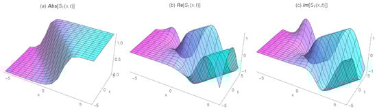
Figure 1. The 3D wave profiles for the absolute, real, and imaginary values of the dark (kink) soliton solution for $b=0.9$, $c=-0.3$, $s=1.5,k=1,{\vartheta }_0=0.2,{\epsilon }_1={\epsilon }_2=1,{\epsilon }_3=1.2,\Omega =0.5.$

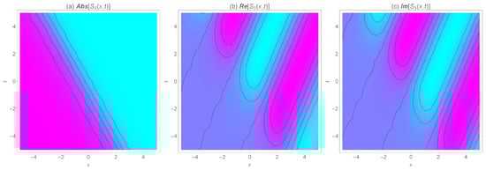
Figure 2. The 2D density of the wave surfaces for the absolute, real, and imaginary values of the dark (kink) soliton solution for $b=0.9,c=-0.3,s=1.5,k=1,{\vartheta }_0=0.2,{\epsilon }_1=1,{\epsilon }_2=1,{\epsilon }_3=1.2,\Omega =0.5.$

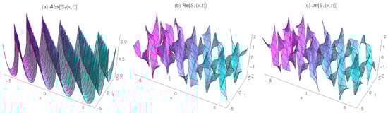
Figure 3. The 3D wave profiles for the absolute, real, and imaginary values of the periodic soliton solution for $b=0.9,c=0.3,$$s=1.5,k=1,{\vartheta }_0=0.2,{\epsilon }_1={\epsilon }_2=1,{\epsilon }_3=1.2,\Omega =0.5.$

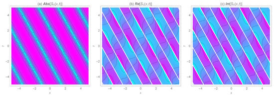
Figure 4. The 2D density of the wave surfaces for the absolute, real, and imaginary values of the periodic soliton solution for $b=0.9$, $4c=-0.3$, $s=1.5,k=1,{\vartheta }_0=0.2,{\epsilon }_1=1,{\epsilon }_2=1,{\epsilon }_3=1.2,\Omega =0.5.$

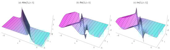
Figure 5. The 3D wave profiles for the absolute, real, and imaginary values of the singular kink-like soliton solution for $b=0.9,$$c=-0.3,s=1.5,k=1,{\vartheta }_0=0.2,{\epsilon }_1=1,{\epsilon }_2=1,{\epsilon }_3=1.2,\Omega =0.5.$

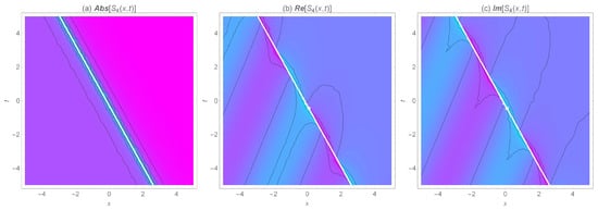
Figure 6. The 2D density of the wave surfaces for the absolute, real, and imaginary values of the singular kink soliton solution for $b=0.9,c=-0.3,s=1.5,k=1,{\vartheta }_0=0.2,{\epsilon }_1=1,{\epsilon }_2=1,{\epsilon }_3=1.2,\Omega =0.5.$

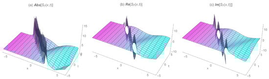
Figure 7. The 3D wave profiles for the absolute, real, and imaginary values of the singular kink soliton solution for $b=0.9,c=-0.3,$$s=1.5,k=1,{\vartheta }_0=0.2,{\epsilon }_1=1,{\epsilon }_2=1,{\epsilon }_3=1.2,\Omega =0.5.$

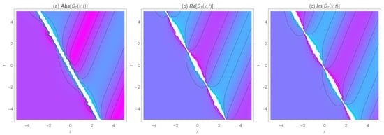
Figure 8. The 2D density of the wave surfaces for the absolute, real, and imaginary values of the singular kink-like soliton solution for $b=0.9,c=-0.3,s=1.5,k=1,{\vartheta }_0=0.2,{\epsilon }_1=1,{\epsilon }_2=1,{\epsilon }_3=1.2,\Omega =0.5.$

References

- Hasegawa, A.; Kodama, Y. Solitons in Optical Communications; Oxford University Press: New York, NY, USA, 1995. [Google Scholar]
- Agrawal, G.P. Nonlinear Fiber Optics, 5th ed.; Springer: New York, NY, USA, 2013. [Google Scholar]
- Arshad, M.; Seadawy, A.R.; Lu, D. Exact bright-dark solitary wave solutions of the higher-order cubic-quintic nonlinear Schrodinger equation and its stability. Optik 2017, 128, 40–49. [Google Scholar] [CrossRef]
- Arshad, M.; Seadawy, A.R.; Lu, D.; Wang, J. Optical soliton solutions of unstable nonlinear Schrödinger dynamical equation and stability analysis with applications. Optik 2018, 157, 597–605. [Google Scholar] [CrossRef]
- Az-Zo’bi, E.A. Modified Laplace decomposition method. World Appl. Sci. J. 2012, 18, 1481–1486. [Google Scholar]
- Az-Zo’bi, E.A. An Approximate Analytic Solution for Isentropic Flow by An Inviscid Gas Equations. Arch. Mech. 2014, 66, 203–212. [Google Scholar]
- Pellegrino, E.; Pezza, L.; Pitolli, F. A collocation method in spline spaces for the solution of linear fractional dynamical systems. Math. Comput. Simul. 2020, 176, 266–278. [Google Scholar] [CrossRef] [Green Version]
- Goswami, A.; Rathore, S.; Singh, J.; Kumar, D. Analytical study of fractional nonlinear Schrödinger equation with harmonic oscillator. Discret. Contin. Dyn. Syst. S 2021. [Google Scholar] [CrossRef]
- Arshad, S.; Siddiqui, A.M.; Sohail, A.; Maqbool, K.; Li, Z.-W. Comparison of optimal homotopy analysis method and fractional homotopy analysis transform method for the dynamical analysis of fractional order optical solitons. Adv. Mech. Eng. 2021, 9, 1687814017692946. [Google Scholar] [CrossRef] [Green Version]
- Az-Zo’bi, E.A.; Al Dawoud, K.; Marashdeh, M.F. Numeric-analytic solutions of mixed-type systems of balance laws. Appl. Math. Comput. 2015, 265, 133–143. [Google Scholar] [CrossRef]
- Az-Zo’bi, E.A.; Al-Amr, M.O.; Yıldırım, A.; AlZoubi, W.A. Revised reduced differential transform method using Adomian’s polynomials with convergence analysis. Math. Eng. Sci. Aerosp. 2020, 11, 827–840. [Google Scholar]
- Akinyemi, L.; Iyiola, O.S. A reliable technique to study nonlinear time-fractional coupled Korteweg-de Vries equations. Adv. Differ. Equ. 2020, 2020, 169. [Google Scholar] [CrossRef] [Green Version]
- Rani, M.; Bhatti, H.S.; Singh, V. Exact solitary wave solution for higher order nonlinear Schrodinger equation using He’s variational iteration method. Opt. Eng. 2017, 56, 116103. [Google Scholar] [CrossRef]
- Akgül, A.; Bonyah, E. Reproducing kernel Hilbert space method for the solutions of generalized Kuramoto–Sivashinsky equation. J. Taibah Univ. Sci. 2019, 13, 661–690. [Google Scholar] [CrossRef] [Green Version]
- Akinyemi, L.; Iyiola, O.S. Exact and approximate solutions of time-fractional models arising from physics via Shehu transform. Math. Meth. Appl. Sci. 2020, 43, 7442–7464. [Google Scholar] [CrossRef]
- Az-Zo’bi, E.A. A reliable analytic study for higher-dimensional telegraph equation. J. Math. Comput. Sci. 2018, 18, 423–429. [Google Scholar] [CrossRef]
- Senol, M.; Iyiola, O.S.; Daei Kasmaei, H.; Akinyemi, L. Efficient analytical techniques for solving time-fractional nonlinear coupled Jaulent-Miodek system with energy-dependent Schrödinger potential. Adv. Differ. Equ. 2019, 2019, 1–21. [Google Scholar] [CrossRef]
- Kudryashov, N.A. One method for finding exact solutions of nonlinear differential equations. Commun. Nonlinear Sci. Numer. Simul. 2012, 17, 2248–2253. [Google Scholar] [CrossRef] [Green Version]
- Kudryashov, N.A. Mathematical model of propagation pulse in optical fiber with power nonlinearities. Optik 2020, 212, 164750. [Google Scholar] [CrossRef]
- Kudryashov, N.A. Method for finding highly dispersive optical solitons of nonlinear differential equations. Optik 2020, 206, 163550. [Google Scholar] [CrossRef]
- Az-Zo’bi, E.A.; Alzoubi, W.A.; Akinyemi, L.; Şenol, M.; Masaedeh, B.S. A variety of wave amplitudes for the conformable fractional (2 + 1)-dimensional Ito equation. Mod. Phys. Lett. B 2021, 35, 2150254. [Google Scholar] [CrossRef]
- Salas, A.H.; Martinez, H.L.J.; Ocampo, R.D.L. New Solutions for the Generalized BBM Equation in terms of Jacobi and Weierstrass Elliptic Functions. Abstr. Appl. Anal. 2021, 2021, 5513266. [Google Scholar] [CrossRef]
- Rezazadeh, H.; Adel, W.; Eslami, M.; Tariq, K.U.; Mirhosseini-Alizamini, S.M.; Bekir, A.; Chu, Y.-M. On the optical solutions to nonlinear Schrödinger equation with second-order spatiotemporal dispersion. Open Phys. 2021, 19, 111–118. [Google Scholar] [CrossRef]
- Jia, T.-T.; Chai, Y.-Z.; Hao, H.-Q. Multi-soliton solutions and Breathers for the generalized coupled nonlinear Hirota equations via the Hirota method. Superlattices Microstruct. 2017, 105, 172–182. [Google Scholar] [CrossRef]
- Akinyemi, L.; Senol, M.; Iyiola, O.S. Exact solutions of the generalized multidimensional mathematical physics models via sub-equation method. Math. Comput. Simul. 2021, 182, 211–233. [Google Scholar] [CrossRef]
- Boudoue-Hubert, M.; Nestor, S.; Douvagai; Betchewe, G.; Biswas, A.; Khan, S.; Belic, M. Dispersive solitons in optical metamaterials having parabolic form of nonlinearity. Optik 2018, 179, 1009–1018. [Google Scholar] [CrossRef]
- Akinyemi, L.; Şenol, M.; Rezazadeh, H.; Ahmad, H.; Wang, H. Abundant optical soliton solutions for an integrable (2+1)-dimensional nonlinear conformable Schrödinger system. Results Phys. 2021, 104177. [Google Scholar] [CrossRef]
- Şenol, M. New analytical solutions of fractional symmetric regularized-long-wave equation. Rev. Mex. Fis. 2020, 66, 297–307. [Google Scholar] [CrossRef]
- Ekici, M.; Sonmezoglu, A. Optical solitons with Biswas-Arshed equation by the extended trial function method. Optik 2019, 177, 13–20. [Google Scholar] [CrossRef]
- Ghanbari, B.; Inc, M. A new generalized exponential rational function method to find exact special solutions for the resonance nonlinear Schrödinger equation. Eur. Phys. J. Plus 2018, 133, 142. [Google Scholar] [CrossRef]
- Tikhov, S.V.; Valovik, D.V. Maxwell’s equations with arbitrary self-action nonlinearity in a waveguiding theory: Guided modes and asymptotic of eigenvalues. J. Math. Anal. Appl. 2019, 479, 1138–1157. [Google Scholar] [CrossRef]
- Valovik, D.V. On the existence of infinitely many nonperturbative solutions in a transmission eigenvalue problem for nonlinear helmholtz equation with polynomial nonlinearity. Appl. Math. Model. 2018, 53, 296–309. [Google Scholar] [CrossRef]
- Zahran, E.H.M.; Khater, M.M.A. Modified extended tanh-function method and its applications to the Bogoyavlenskii equation. Appl. Math. Model. 2016, 40, 1769–1775. [Google Scholar] [CrossRef]
- Kudryashov, N.A. Simplest equation method to look for exact solutions of nonlinear differential equations. Chaos Solitons Fractals 2005, 24, 1217–1231. [Google Scholar] [CrossRef] [Green Version]
- Kudryashov, N.A. Exact solitary waves of the Fisher equation. Phys. Lett. A 2005, 342, 99–106. [Google Scholar] [CrossRef]
- Jawad, A.J.; Petkovic, M.D.; Biswas, A. Modified simple equation method for nonlinear evolution equations. Appl. Math. Comput. 2010, 217, 869–877. [Google Scholar]
- Choudhuri, A.; Porsezian, K. Dark-in-the-Bright solitary wave solution of higher-order nonlinear Schrödinger equation with non-Kerr terms. Opt. Commun. 2012, 285, 364–367. [Google Scholar] [CrossRef]
- Arshad, M.; Seadawy, A.R.; Lu, D. Study of soliton solutions of higher-order nonlinear Schrödinger dynamical model with derivative non-Kerr nonlinear terms and modulation instability analysis. Results Phys. 2019, 13, 102305. [Google Scholar] [CrossRef]
- Khater, M.M.A.; Attia, R.A.M.; Abdel-Aty, A.-H.; Abdou, M.A.; Eleuch, H.; Lu, D. Analytical and semi-analytical ample solutions of the higher-order nonlinear Schrödinger equation with the non-Kerr nonlinear term. Results Phys. 2020, 16, 103000. [Google Scholar] [CrossRef]
- Zayed, E.M.E.; Al-Nowehy, A.-G. Many new exact solutions to the higher-order nonlinear Schrodinger equation with derivative non Kerr nonlinear terms using three different techniques. Optik 2017, 143, 84–103. [Google Scholar] [CrossRef]
- Sharma, V.K.; De, K.K.; Goyal, A. Solitary wave solutions of higher-order nonlinear Schrödinger equation with derivative non-Kerr nonlinear terms. Workshop Recent Adv. Photonics WRAP 2013. [Google Scholar] [CrossRef]
- Az-Zo’bi, E.A.; AlZoubi, W.A.; Akinyemi, L.; Şenol, M.; Alsaraireh, I.W.; Mamat, M. Abundant closed-form solitons for time-fractional integro–differential equation in fluid dynamics. Opt. Quant. Electron. 2021, 53, 132. [Google Scholar] [CrossRef]
- Darwish, A.; El-Dahab, E.A.; Ahmed, H.; Arnous, A.H.; Ahmed, M.S.; Biswas, A.; Guggilla, P.; Yıldırım, Y.; Mallawi, F.; Belic, M.R. Optical solitons in fiber Bragg gratings via modified simple equation. Optik 2020, 203, 163886. [Google Scholar] [CrossRef]
- Al-Amr, M.O.; Rezazadeh, H.; Ali, K.K.; Korkmazki, A. N1-soliton solution for Schrödinger equation with competing weakly nonlocal and parabolic law nonlinearities. Commun. Theor. Phys. 2020, 72, 065503. [Google Scholar] [CrossRef]
- Islam, M.N.; Asaduzzaman, M.; Ali, M.S. Exact wave solutions to the simplified modified Camassa-Holm equation in mathematical physics. AIMS Math. 2020, 5, 26–41. [Google Scholar] [CrossRef]
- El-Sheikh, M.M.; Ahmed, H.M.; Arnous, A.H.; Rabie, W.B.; Biswas, A.; Alshomrani, A.S.; Ekici, M.; Zhou, Q.; Belic, M.R. Optical solitons in birefringent fibers with Lakshmanan-Porsezian-Daniel model by modified simple equation. Optik 2019, 192, 162899. [Google Scholar] [CrossRef]
- Az-Zo’bi, E.A. New kink solutions for the van der Waals p-system. Math. Methods Appl. Sci. 2019, 42, 6216–6226. [Google Scholar] [CrossRef]
- Yıldırım, Y. Optical solitons to Kundu–Mukherjee–Naskar model in birefringent fibers with modified simple equation approach. Optik 2019, 184, 121–127. [Google Scholar] [CrossRef]
- Az-Zo’bi, E.A. Peakon and solitary wave solutions for the modified Fornberg-Whitham equation using simplest equation method. Int. J. Math. Comput. Sci. 2019, 14, 635–645. [Google Scholar]
- Kazi, S.; Hossain, A.K.M.; Akbar, M.A.; Wazwaz, A.-M. Closed form solutions of complex wave equations via the modified simple equation method. Cogent Phys. 2017, 4, 1312751. [Google Scholar] [CrossRef]
- Irshad, A.; Mohyud-Din, S.T.; Ahmed, N.; Khan, U. A New Modification in Simple Equation Method and its applications on nonlinear equations of physical nature. Results Phys. 2017, 7, 4232–4240. [Google Scholar] [CrossRef]
Publisher’s Note: MDPI stays neutral with regard to jurisdictional claims in published maps and institutional affiliations. |
© 2021 by the authors. Licensee MDPI, Basel, Switzerland. This article is an open access article distributed under the terms and conditions of the Creative Commons Attribution (CC BY) license (https://creativecommons.org/licenses/by/4.0/).