Multi-Output Soft Sensor with a Multivariate Filter That Predicts Errors Applied to an Industrial Reactive Distillation Process

Abstract

The paper deals with the problem of developing a multi-output soft sensor for the industrial reactive distillation process of methyl tert-butyl ether production. Unlike the existing soft sensor approaches, this paper proposes using a soft sensor with filters to predict model errors, which are then taken into account as corrections in the final predictions of outputs. The decomposition of the problem of optimal estimation of time delays is proposed for each input of the soft sensor. Using the proposed approach to predict the concentrations of methyl sec-butyl ether, methanol, and the sum of dimers and trimers of isobutylene in the output product in a reactive distillation column was shown to improve the results by 32%, 67%, and 9.5%, respectively.

1. Introduction

As the size and complexity of industrial systems increases, there is a need to accurately measure most process variables. Unfortunately, not all variables can be accurately measured using online hard sensors. For certain variables, such as concentration or density, the only accurate measurements can be obtained by manually taking samples and analyzing them in a laboratory. One solution to this problem is the development of soft sensors, which take the easy-to-measure variables and create models to predict the hard-to-measure variables [1].

All soft sensor systems consist of a process model that takes the easy-to-measure variables and provides an estimate of the hard-to-measure variables. These models can be constructed using methods ranging from linear regression to principal component analysis and support vector machines. Although the main focus has been on the development of the soft sensor models [2,3,4,5], advanced soft sensor systems have also a bias update term that can take any slowly sampled information to update the soft sensor prediction [1]. This bias update term is normally designed as some function of the difference between the predicted and measured values [6]. Of note, it should be mentioned that the measured values are often sampled very slowly and with considerable time delay. This means that during the points at which there are no updates, the previously available bias value is used. When such a system is properly designed, it can provide good tracking of the process, i.e., the predicted and measured values are close to each other.

Recently, it has been suggested that instead of only using the available slowly sampled data for updating the bias term, it should be possible to also model the historical errors and use them to predict the future errors [7]. It has been shown that such an approach can improve the overall performance of the soft sensor system. However, there still remain issues with how best to model and implement this predictive bias update term. Furthermore, there are issues with incorporating time delays into this approach since they will greatly increase the size of the required search space.

Therefore, this paper will examine the development of a predictive bias update term for a nonlinear system using dimension reduction. The proposed approach will be tested using data from an industrial reactive distillation column that produces methyl tert-butyl ether (MTBE).

2. Background

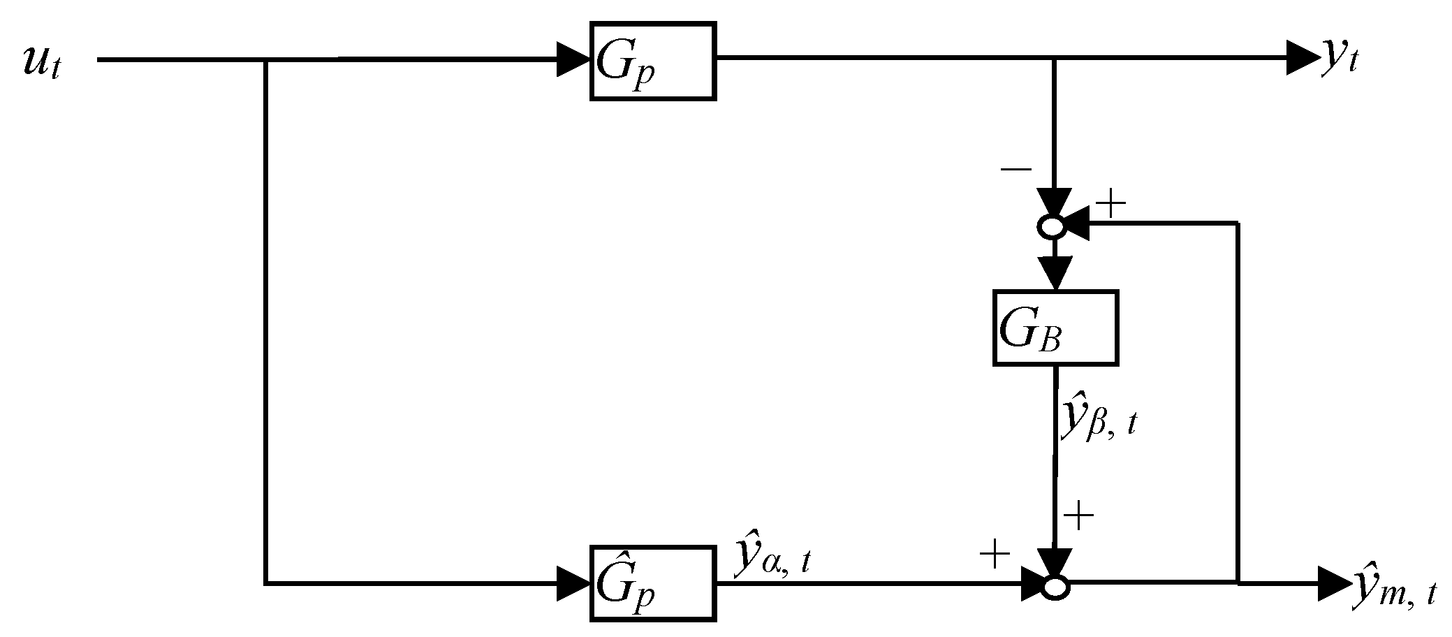
Consider the soft sensor system shown in Figure 1, where u_t is the input, y_t is the measured (true) output, ${\widehat{y}}_{m,t}$ the predicted soft sensor value, ${\widehat{y}}_{\alpha ,t}$ and ${\widehat{y}}_{\beta ,t}$ are intermediate soft sensor values, G_p is the true process, ${\widehat{G}}_p$ is the soft sensor process model, and G_B is the bias update term. It can be noted that purpose of the bias update term is to take the information from the measured values and correct the output of the soft sensor system. This comes primarily from the unknown disturbances and the inherent plant-model mismatch.

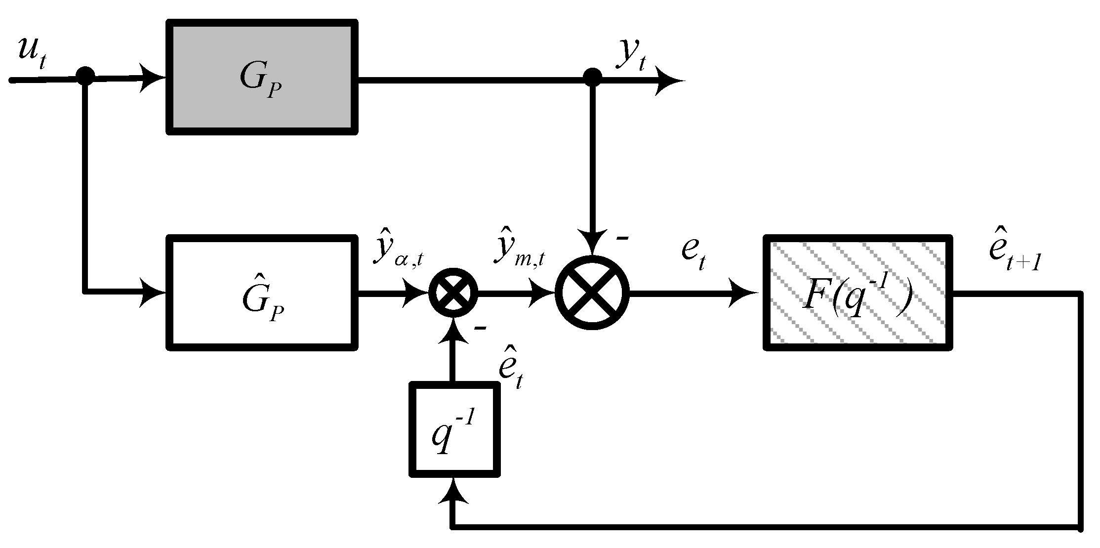
Another approach to this problem is to re-arrange the bias update term so that it contains a predictive model that can predict the errors between the measured and predicted values. This re-arrangement is shown in Figure 2, where the predicted value from the soft sensor is corrected based on the modeled errors of the system. The question becomes how to design this model so that the best predictions can be obtained.

For prediction of time series, the Box-Jenkins methodology is traditionally used, according to which the time series model is found in the class of autoregressive-moving average (ARMA) models, i.e., is considered a rational algebraic function of the backward shift operator. The flexibility of the ARMA class makes it possible to find parsimonious models, i.e., the adequacy of the evaluated model is achieved with a small number of estimated parameters. Since this property is especially important for empirical models, the Box-Jenkins methodology is widely used to solve various practical problems. This approach is adopted in this paper.

In industrial processes, where it is desired to implement the model on programmable logic control (PLC) units, the complexity of the model ${\widehat{G}}_p$ can be an issue. Therefore, this paper will consider a simple model for ${\widehat{G}}_p$ of the form

y_t = b₀ + bx_t + e_t

(1)

where b are the parameters to be estimated and x_t is the input(s). Model (1) can be improved by taking into account possible delays of the output variables relative to inputs. Consider the following model for a multi-output soft sensor

y_{t, m} = b_m u_m (t, τ_m) + e_{t, m}

(2)

where t = 1, 2, …, n; m = 1, 2, 3 (the number of outputs m is given by the industrial production team and reflecting the key quality indices of MTBE product). Vector b_m = (b_{m, 1}, b_{m, 2}, …, b_{m, 10}) is a row vector of unknown coefficients; τ_m = (τ_{m, 1}, τ_{m, 2}, …, τ_{m, 10}) is a row vector of unknown time delays; u_m (t, τ_m) = (u_{t, m, 1}, u_{t, m, 2}, …, u_{t, m, 10})^T; u_{t, m, k} is the measurement of the x_k value at time t − τ_{m, k} with k = 1, 2, …, 10. Please note that it has been assumed here that the maximal time delay is 10 samples and justified from the industrial process dynamics point of view. However, it can easily be extended to arbitrary values.

Solving model (2) by minimizing the mean squared error (MSE) gives an estimate for the unknown parameters ${\widehat{b}}_m$ and ${\widehat{\tau }}_m$. The MSE depends not only on the coefficients b_m, but also on the delays τ_m, i.e.,

$$D_{em}(b_m {\tau }_m)=\frac{1}{n}{\displaystyle \sum _{t=1}^n{\left\{y_{tm}- b_m{u}_m(t, {\tau }_m)\right\}}^2}, m = 1, 2, 3$$

(3)

Thus,

$$({\widehat{b}}_m, {\widehat{\tau }}_m)=\mathbf{arg}\underset{b_m, {\tau }_m}{\min }{D}_{em}(b_m, {\tau }_m).$$

(4)

Please note that if $D_{em}(b_m^{*}, {\tau }_m^{*})=\underset{b_m, {\tau }_m}{\min }{D}_{em}(b_m, {\tau }_m)$, than $D_{em}(b_m^{*}, {\tau }_m^{*})=\underset{b_m}{\min }{D}_{em}(b_m, {\tau }_m^{*}).$

Consequently,

$$\underset{b_m, {\tau }_m}{\min }{D}_{em}(b_m, {\tau }_m)=\underset{ {\tau }_m}{\min }\left\{\underset{b_m}{\min }{D}_{em}(b_m, {\tau }_m)\right\}=\underset{ {\tau }_m}{\min }{D}_{em}({\widehat{b}}_m, {\tau }_m)$$

(5)

Furthermore, the estimates ${\widehat{b}}_m$ are found using standard regression analysis which gives

$${\widehat{b}}_m={\left\{{\left(U_m^T{U}_m\right)}^{-1}{U}_m^T{Y}_m\right\}}^{\mathrm{T}}, m=1, 2, 3$$

(6)

where Y_m is the m-th column of the matrix Y; U_m is a matrix with dimension n × 10, whose t-th row is the row u_m (t, τ_m)^T.

Since all variables are measured at discrete moments in time, the gradient descent methods cannot be directly applied to minimize the objective function $D_{em}({\widehat{b}}_m, {\tau }_m)$ for the argument τ_m. However, this difficulty can be avoided by calculating D_em for any values of the elements of the vector τ_m by interpolating between the nearby nodes of the discrete grid. Interpolation with a large search space dimension is a difficult problem. Among the various characteristics of the algorithms used, such properties as visibility and relative simplicity come to the fore. Therefore, in this situation, the most preferable is the polynomial interpolation.

2.1. Error Modeling

If the e_{t, m} error were known at time t − 1, then using Equation (2), it would be possible to predict the y_{t, m} variable with absolute accuracy. Unfortunately, the e_{t, m} error is not known in advance, but it can be predicted using any statistical patterns found in the sequence e_{1, m}, e_{2, m}, …. This error prediction can be used as a correction to model (2) as shown in Figure 2, therefore improving the prediction accuracy of the y_t,m output variable. To evaluate a predictive model for the sequence e_{1, m}, e_{2, m} …, let us consider the class of ARMA models. Let us introduce the predicted process as the output of an invertible linear filter, called a shaping filter, driven by white noise, i.e., a process with a constant spectral density. In this case, the transfer function of the shaping filter is considered a rational algebraic function of the backward shift operator, i.e.,

$$e_t=\frac{{\displaystyle \prod _{l=1}^{N_n}(1-H_l{q}^{-1})}}{{\displaystyle \prod _{k=1}^{N_d}(1-G_k{q}^{-1})}}{\epsilon }_t$$

(7)

where ε_t and e_t are values of the input and output processes of the shaping filter at time t; N_n is the order of the moving average; N_d is the order of the autoregressive component; H_l, G_k are constants (generally speaking, complex-valued); and $q^{-1}$ is the backshift operator. The stationarity and invertibility conditions, which are necessary to predict the e_t process, are [8]

$$\left|G_k\right|<1, k=1, \dots , N_d;\hspace{1em}\left|H_l\right|<1, l=1, \dots , N_n$$

(8)

The flexibility of the ARMA class provides the possibility of finding parsimonious models, i.e., the adequacy of the constructed model is achieved with a relatively small number of estimated parameters. Since this property is especially important for empirical models, the models with the structure given in Equation (7) and their variants are widely used for solving practical problems.

The filter for predicting the e_t process can be found using the prediction error method (PEM) [9]. Expanding the brackets in Equation (7) gives

$$e_t=\frac{(1-{\theta }_1{q}^{-1}-\dots -{\theta }_{N_n}{q}^{-N_n})}{(1-{\eta }_1{q}^{-1}-\dots -{\eta }_{N_d}{q}^{-N_d})}{\epsilon }_t$$

(9)

where θ_l and η_k are the model parameters. It is assumed that the polynomials in the numerator and denominator have no common roots, since otherwise it would be possible to reduce the common multipliers in the numerator and denominator of Equation (7).

The PEM function finds the parameter values that minimize the predictive MSE of the e_t process for given polynomial orders (N_n, N_d) and the initial estimates of the parameters θ_l and η_k. It is possible to choose suitable orders of the polynomials based on sample estimations of the spectral density of the considered process. Recall that the frequency response of the shaping filter is the value of Equation (7) on a circle of unit radius centered on the origin and the spectral density S(ω) of the output process e_t is equal to the product of the variance of the input process and the square of the frequency response modulus, i.e., [10]

$$S(\omega )={\sigma }_{\epsilon }^2\frac{{\displaystyle \prod _{l=1}^{N_n}(1-H_l{e}^{-j\omega })}}{{\displaystyle \prod _{k=1}^{N_d}(1-G_k{e}^{-j\omega })}}\frac{{\displaystyle \prod _{l=1}^{N_n}(1-{\overline{H}}_l{e}^{j\omega })}}{{\displaystyle \prod _{k=1}^{N_d}(1-{\overline{G}}_k{e}^{j\omega })}},$$

(10)

where ${\sigma }_{\epsilon }^2$ is the variance of random process ε_t and H_l and G_k are the complex conjugates of the constants H_l and G_k. Furthermore, since we desire that our filter be invertible, it follows that for the model

$${\epsilon }_t=\frac{{\displaystyle \prod _{k=1}^{N_d}(1-G_k{q}^{-1})}}{{\displaystyle \prod _{l=1}^{N_n}(1-H_l{q}^{-1})}} e_t$$

(11)

the e_t process is invertible if the absolute values of all the H_l constants are less than one. Similarly, if the absolute values of all the G_k constants is less than one, then the e_t process is stationary [8]. Thus, although multiple processes can have the same spectral density, there is only one that is both stationary and invertible.

Once the general model has been obtained, we can rewrite it as an infinite impulse response model, i.e.,

$$e_t={\epsilon }_t+{\displaystyle \sum _{k=1}^{\infty }{\psi }_k{\epsilon }_{t-k}}$$

(12)

where ψ is an impulse response coefficient. Since we know that the general model converges [8], it follows that we only need a finite number of terms in Equation (12). Furthermore, we note that

$$e_{t-i}={\epsilon }_{t-i}+{\displaystyle \sum _{k=1}^{\infty }{\psi }_k{\epsilon }_{t-i-k}}$$

(13)

which implies that for any positive i the random variables ε_t and e_t−i are uncorrelated (since the process ε_t is white noise). Therefore, successively multiplying both sides of Equation (12) by the values of the corresponding process at delays i and taking expectations, we obtain equations for finding the initial estimates of the parameters that involve the covariances of the errors for different lags [10]. Obviously, since the true covariances are not known, they will need to be replaced by the sample estimates. This method of estimating the coefficients does not lead to too large error as long as the absolute values of the parameters of model (7) are not too close to the boundary of unit circle centered on the origin. Thus, it is possible to design the required filter.

2.2. Filter Design

Let e_t = (e_{t, 1}, e_{t, 2}, …, e_{t, N})^T be an N-dimensional stationary process of the soft sensor’s errors whose shaping filter transfer matrix is F₀(q⁻¹), i.e.,

e_t = F₀(q⁻¹)ε_t

(14)

where q⁻¹ is the backshift operator; ε_t = (ε_{t, 1}, ε_{t, 2}, …, ε_{t, N})^T is an N-dimensional vector of white noise; and F₀(q⁻¹) = [f_km(q⁻¹)] is an N $\times$ N matrix function, whose entries denoted as f_km(q⁻¹) are the rational transfer function from ε_t,m to e_{t, k}. Thus, it is desired to construct the filter that will predict e_t+1 given the past values.

Let P(q⁻¹) be the desired one-step ahead predictor transfer matrix, ${\widehat{e}}_{t+1}$ = P(q⁻¹)e_t the prediction of the vector e_t+1 at time t, and ${\tilde{\epsilon }}_{t+1}$ = e_t+1 − ${\widehat{e}}_{t+1}$ the error of the prediction obtained with the aid of the filter P(q⁻¹). Then

$${\tilde{\epsilon }}_t=e_t-{\widehat{e}}_t=e_t-q^{-1}{\widehat{e}}_{t+1}=e_t-q^{-1}\mathit{P}\left(q^{-1}\right)e_t=[I_N-q^{-1}\mathit{P}(q^{-1}\left)\right]e_t$$

(15)

where I_N is identity matrix of order N. Consequently, the filter in the square brackets transforms the initial series into the prediction error series. If the random vector ${\tilde{\epsilon }}_t$ includes components correlated with those of the vector ${\tilde{\epsilon }}_{t-j}$ at some j > 0, we can predict the errors ${\tilde{\epsilon }}_t$ using the known previous errors. Using those predictions as corrections to the ${\tilde{e}}_t$ that were obtained, we could improve the accuracy of the predictions. Hence, in order to maximize the predictor accuracy, we must find a P(q⁻¹) such that the errors ${\tilde{\epsilon }}_t$ are uncorrelated with the errors ${\tilde{\epsilon }}_{t-j}$ at any j > 0 with some nonzero correlation between the components of ${\tilde{\epsilon }}_t$ (i.e., at j = 0) being admissible. In other words, the time series ${\tilde{\epsilon }}_t$ must be N-dimensional white noise. Consequently, I_N − q⁻¹P(q⁻¹) = F₀⁻¹(q⁻¹), from which it follows that P(q⁻¹) = q[I_N − F₀⁻¹(q⁻¹)].

Thus, the predictor transfer matrix P(q⁻¹) can be expressed through the transfer matrix of the shaping filter F₀(q⁻¹). The matrix F₀(q⁻¹) can be found from

G(q⁻¹) = F₀(q⁻¹)F₀^T(q),

(16)

where G(q⁻¹) = [g_km(q⁻¹)], g_km(q⁻¹) is the q-transform of the statistical estimate of the cross-covariance function of the time series e_{t, k} and e_{t, m} (in particular, when m = k, g_mm is a q-transform of the sample covariance function, i.e., the autocovariance generating function (AGF) of the time series e_tm).

The algorithm for finding F₀(q⁻¹) is simplified by decomposing it into N stages. At the kth stage, a shaping filter F_k(q⁻¹) of the k-dimensional process (e_{t, 1}, e_{t, 2}, …, e_{t, k})^T is found. At this stage, the filter F_k−1(q⁻¹), found at the (k−1)th stage, is used in order to transform the matrix G_k(q⁻¹) = F_k(q⁻¹)F_k^T(q) so that its transform contains nonzero elements in only one line, one column, and on the main diagonal. This technique substantially simplifies the procedure of spectral factorization (finding the matrix function F_k(q⁻¹)) [11].

The proposed approach allows us to identify the vector time series transfer matrix without resorting to a complicated phase state representation. This advantage is used to obtain an adequate model with relatively few estimated parameters for the initial time series shaping filter F₀(q⁻¹). Simultaneously, the model for the transfer matrix of the inverse filter F₀⁻¹(q⁻¹), which transforms the initial time series into the white noise, is also found.

The algorithm for constructing both the shaping filter F₀(q⁻¹) and its inverse F₀⁻¹(q⁻¹) is described in [11]. Based on this algorithm, the sequence of prediction errors ${\tilde{\epsilon }}_t$ should be N-dimensional white noise. However, since in practice, the true characteristics of the original process are not known, but only their estimates, containing inevitable statistical errors, in reality, the properties of the sequence ${\tilde{\epsilon }}_t$ can be significantly different from the properties of white noise. Thus, to verify the optimality of the resulting model P(q⁻¹) of the predictive filter, a criterion is needed to test the hypothesis that the process ${\tilde{\epsilon }}_t$ is N-dimensional white noise. To construct such a criterion, we can transform the process ${\tilde{\epsilon }}_t$ in such a way that its spectral density matrix is diagonal. Such a transformation is achieved by means of a rotation of axes in the N-dimensional variable space ${\tilde{\epsilon }}_1, {\tilde{\epsilon }}_2,\cdots ,{\tilde{\epsilon }}_N$ [12]. Since the variances of these variables can be made equal to each other by normalization, without loss of generality, we suppose that spectral density matrix of the noise ${\tilde{\epsilon }}_t$ is an N × N identity matrix I_N.

Consider a univariate sequence ξ_k = ${\tilde{\epsilon }}_{t-j,m}$, where k = jN + m. Please note that each pair couple (j, m) determines one k and each k determines one pair couple (j, m). Consequently, ${\tilde{\epsilon }}_t$ is multivariate white noise if and only if ξ_k is univariate white noise. It is known that the spectral density of univariate white noise is constant [8,13]. Thus, testing the hypothesis that ${\tilde{\epsilon }}_t$ is multivariate white noise is reduced to testing the hypothesis on the constancy of the spectral density of a univariate sequence. This hypothesis can be tested using Kolmogorov’s criterion [14].

Please note that only a time series containing prediction errors is used as the initial information for constructing a predictor with the proposed approach. Information about the model with which the predictions were obtained is not used. Therefore, this approach is applicable to any predictive model that involves errors, regardless of the specific properties of the model used.

2.3. Summary of the Proposed Approach

Thus, the proposed procedure for developing the model can be summarized as follows:

Step 1: Create an initial sample u_t, y_t, t = 1, 2, …, K. If the plant is already functioning then the initial sample consists of the historical values of u_t, y_t. Otherwise, the initial sample is forming during the trial period of the plant. The initial sample is divided into training and testing datasets.

Step 2: Based on the data included in the training sample, the coefficients and delays of the model given by Equation (2) are estimated via solving optimization problem (4).

Step 3: Based on the data included in the training sample, the errors for the model and the corresponding sample spectrum of errors are calculated.

Step 4: Based on the sample spectrum, the order of the ARMA model is selected in order to predict the unknown future error given the known current and past errors.

Step 5: The least squares method is used to find the values of the ARMA model parameters.

Step 6: The ARMA model obtained is used as the predictive filter F(q⁻¹) in the feedback loop of the compensator (bias update term) as shown in Figure 2.

Step 7: If the resulting soft sensor improves the accuracy of the prediction for the test sample then it can be recommended for practical use.

Please note that the obtained predictive filter model can be recommended for further use for the same plant on the data of which it was built. As for the approach, it will certainly be successful if the sequence of errors of the plant is a stationary (or close to it) process. In addition, the class of successful applicability of this approach can be extended to those plants, for whose errors it is possible to find an invertible transformation that brings the sequence of errors to a stationary process. The quality of the developed model should be checked on a test sample that was not used at the stage of the model training.

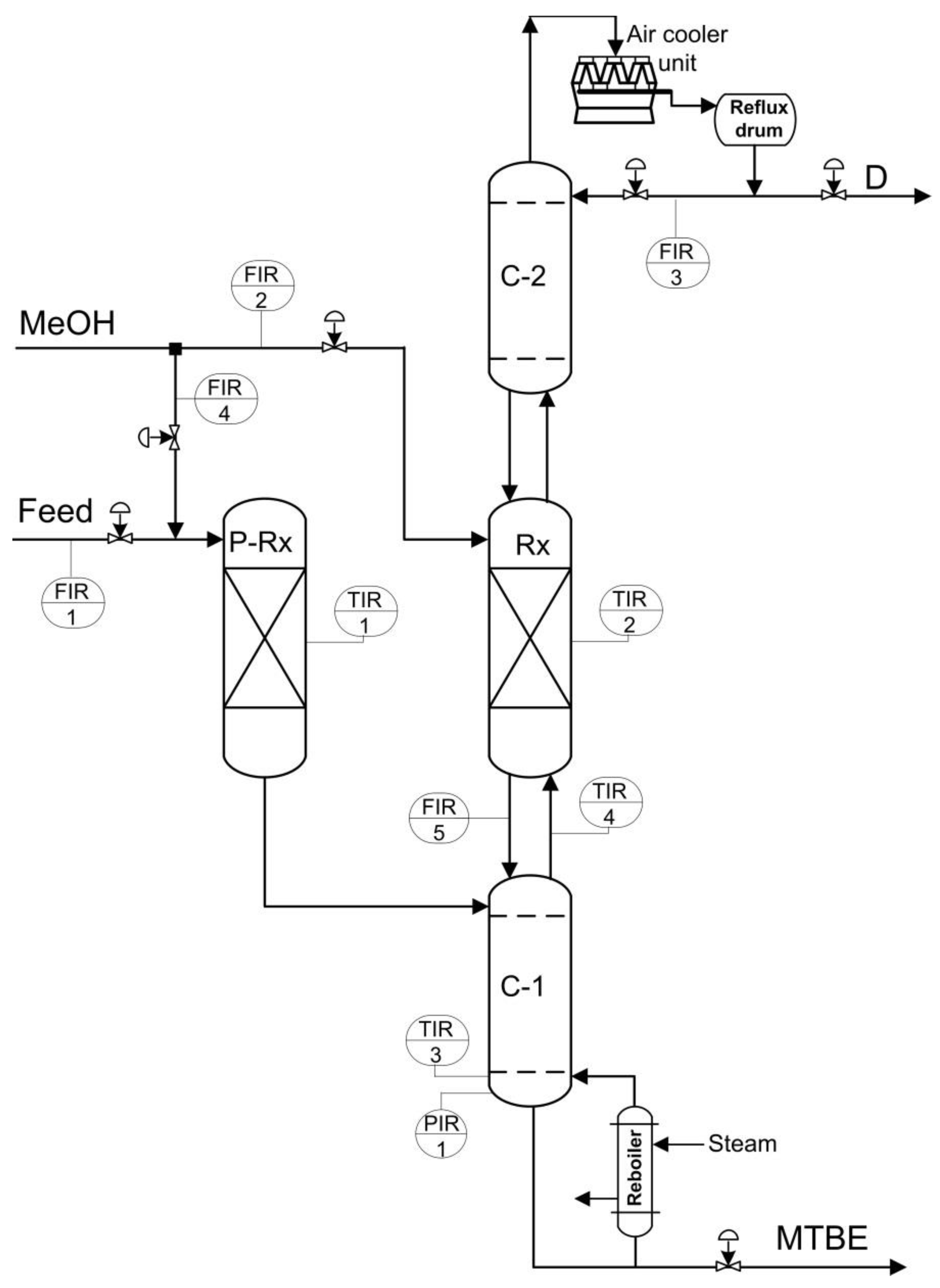
3. Industrial Application of the Proposed Method

Industrial methyl tert-butyl ether (MTBE) production occurs in a reactive distillation unit, as shown in Figure 3. The feed containing isobutylene and methanol (MeOH) enters the column. The distillate (D) is a lean butane-butylene fraction with a certain amount of MeOH. The raffinate is the heavy product MTBE that is withdrawn from the bottom part of the column.

Table 1. Soft sensor input and output variables.

Description of Process Variable	Notation	SS Variable
Feed flowrate, m3/s	FIR−1	x1
MeOH flowrate to Rx, m3/s	FIR-2	x2
Reflux flowrate, m3/s	FIR-3	x3
MeOH flowrate to P-Rx, m3/s	FIR-4	x4
Bottoms flowrate from Rx, m3/s	FIR-5	x5
Bottom pressure, MPa	PIR−1	x6
Temperature in P-Rx, K	TIR−1	x7
Temperature in Rx, K	TIR-2	x8
Bottom temperature, K	TIR-3	x9
Vapor flow temp. from C − 1, K	TIR-4	x10
Concentration of MSBE in MTBE, wt.%	-	y1
Concentration of MeOH in MTBE, wt.%	-	y2
Concentration of DIME in MTBE, wt.%	-	y3

shows the main process variables for the industrial unit. The goal is to develop a soft sensor for the prediction of the concentrations of methyl sec-butyl ether (MSBE), MeOH, and the sum of dimers and trimers of isobutylene (DIME) in the bottom product MTBE.

The measured values of output y_m and input x_k variables at the time moment t are denoted as y_tm, x_tk; m = 1, 2, 3; k = 1, 2, …, 10; and t = 1, 2, …, n. The existing measurements may be used for development of a predictive model of the form

y_t = b₀ + bx_t + e_t, t = 1, 2, …, n

(17)

where y_t = (y_{t, 1}, y_{t, 2}, y_{t, 3})^T; x_t = (x_{t, 1}, x_{t, 2}, …, x_{t, 10})^T; b is a matrix of the model parameters [b_mk] of dimension 3 × 10; b₀ = (b₁, b₂, b₃)^T is a vector of the constant biases; e_t = (e_{t, 1}, e_{t, 2}, e_{t, 3})^T is a vector of the residuals, and the superscript T denotes the transpose. Since Equation (17) can be rewritten as

$$(y_t - \overline{y})=b(x_t-\overline{x})+e_t$$

(18)

where $\overline{y}=\frac{1}{n}{\displaystyle \sum _{t=1}^n{y}_t}$, $\overline{x}=\frac{1}{n}{\displaystyle \sum _{t=1}^n{x}_t}$, then expectations of all the elements of vectors y_t, x_t, and e_t, as well as biases vector b₀, may be considered to be equal to zero without loss of generality.

Although the elements of matrix b are unknown, they are easily estimated using the ordinary least squares (OLS) method, which gives [10]

$$\widehat{b}={\left\{{\left(X^{\mathrm{T}}X\right)}^{-1}{X}^{\mathrm{T}}Y\right\}}^{\mathrm{T}}$$

(19)

where X = [x_tk]; Y = [y_tm]; m = 1, 2, 3; k = 1, 2, …, 10; and t = 1, 2, …, n.

For the training sample containing n = 400 measurements, the following estimates were obtained:

$$\begin{array}{c}\overline{x}=(51.8154\hspace{1em}1.8747\hspace{1em}52.1154\hspace{1em}3.0859\hspace{1em}51.9866\hspace{1em}0.7580\hspace{1em}60.7100\\ {66.4516\hspace{1em}136.3077\hspace{1em}64.5725)}^{\mathrm{T}}\end{array}$$

$$\overline{y}={(0.5440\hspace{1em}0.1461\hspace{1em}0.0595\hspace{1em})}^{\mathrm{T}}$$

$$\begin{array}{c}\widehat{b}=(\begin{array}{ccccc}-0.0151& 0.2383& -0.0342& 0.1401& 0.0476...\\ -0.0173& 0.0794& 0.0281& 0.1191& -0.0171...\\ -0.0080& 0.1118& -0.0061& 0.0537& 0.0134 \dots \end{array}\\ \begin{array}{ccccc}-1.7361& 0.0430& -0.0012& -0.1019& 0.0388\\ 2.9800& -0.0093& -0.0072& -0.1333& 0.0353\\ 0.3490& 0.0215& -0.0011& -0.0467& 0.0098\end{array}).\end{array}$$

The estimated MSE vector for the model (17) is (0.0094 0.0095 0.0021)^T, while the vector of sample estimates of variances of the output variables is (0.0321 0.0184 0.0047)^T.

Let $R_m^2$ be a sample estimate of the coefficient of determination, i.e., the estimate of a fraction of variance of the dependent variable y_m explained by model (18), i.e.,

$$R_m^2=1-\frac{D_{e,m}}{D_m}$$

(20)

where D_m is a sample estimate of the variance of the output variable y_m, D_{e, m} is the mean squared value of the e_{t, m} errors, and m = 1, 2, 3. This gives $R_1^2$ = 0.7061, $R_2^2$ = 0.4822, and $R_3^2$ = 0.5467.

Assuming a sampling time of one hour, the estimates of the delay vector ${\widehat{\tau }}_1$ for predicting the output variable y₁ is

$${\widehat{\tau }}_1=(4.83\hspace{1em}0\hspace{1em}2.00\hspace{1em}5.00\hspace{1em}1.83\hspace{1em}0\hspace{1em}2.00\hspace{1em}0.83\hspace{1em}1.00\hspace{1em}2.00)$$

and the estimate of the coefficient vector is equal to

$${\widehat{b}}_1=(0.0002\hspace{1em}0.1341-0.0360\hspace{1em}0.0064\hspace{1em}0.0451-2.3289\hspace{1em}0.0519-0.0029-0.0819\hspace{1em}0.0442)$$

with D_{e, 1}(${\widehat{b}}_1$, ${\widehat{\tau }}_1$) = 0.0091.

Similarly, for variables y₂ and y₃, we obtain

$${\widehat{\tau }}_2=(0.33\hspace{1em}0.33\hspace{1em}1.67\hspace{1em}4.50\hspace{1em}0.50\hspace{1em}0.67\hspace{1em}0.33\hspace{1em}0.50\hspace{1em}0.50\hspace{1em}1.67)$$

$${\widehat{b}}_2=(-0.0263\hspace{1em}0.1481\hspace{1em}0.0315\hspace{1em}0.1947-0.0168\hspace{1em}3.4223-0.0064-0.0092-0.1513\hspace{1em}0.0385); D_2({\widehat{b}}_2, {\widehat{\tau }}_2)=0.0088$$

$${\widehat{\tau }}_3=(4.17\hspace{1em}0\hspace{1em}0.83\hspace{1em}4.33\hspace{1em}0.83\hspace{1em}0.50\hspace{1em}2.00\hspace{1em}0.67\hspace{1em}0.83\hspace{1em}1.00)$$

$${\widehat{b}}_3=(-0.0021\hspace{1em}0.0811-0.0070\hspace{1em}-0.0016\hspace{1em}0.0130\hspace{1em}0.3795\hspace{1em}0.0259-0.0015-0.0455\hspace{1em}0.0098); D_3({\widehat{b}}_3, {\widehat{\tau }}_3)=0.0020$$

The sample estimate of the coefficient of determination to predict the output variable y_m denoted by $R_{Lm}^2$ is $R_{L1}^2$ = 0.7160; $R_{L2}^2$ = 0.5200; $R_{L3}^2$ = 0.5726.

The effect of delay accounting was evaluated on a test sample containing 167 measurements. As a result, the MSE of the predictions of output variables y₁, y₂ and y₃ decreased by 23%, 10%, and 3%, respectively.

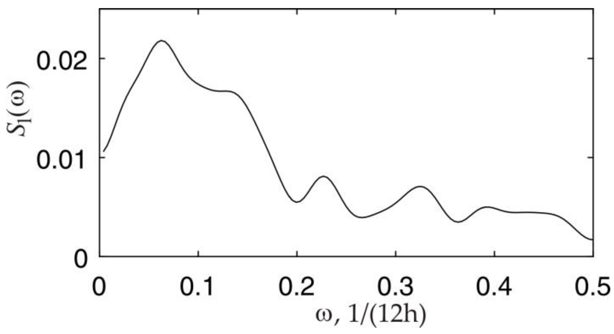
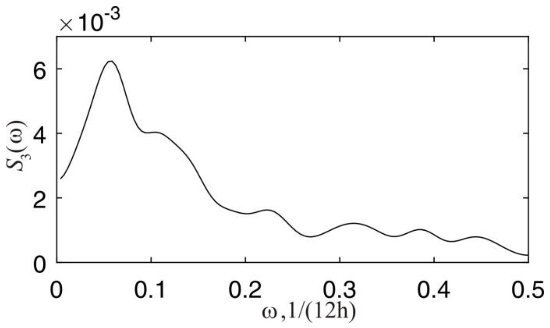
Now, let us consider modeling the error term. From the spectral density of the errors for e_{t, 1} and e_{t, 3} shown in Figure 4 and Figure 5, it can be seen that the maximum within the interval [0, 0.5] Hz indicates the presence in the denominator of the spectral density function S(ω) a factor (1 − Ge^−jω) with a complex-valued constant G. Since the sampling time is equal to 12 h, the frequency unit 1/(12 h) is used instead of Hz. However, for the practical application of the filter given by Equation (9), it is necessary that all the coefficients be real [8]. Therefore, the denominator of density S(ω) must contain a factor (1 − $\overline{G}$e^−jω) along with a factor (1 − Ge^−jω). If the frequency response models for e_{t, 1} and e_{t, 3} processes are limited to these two factors (assuming the numerator is equal to one), then the corresponding spectral density of the second-order autoregressive process approximates well the sample estimates of the spectrum of e_{t, 1} and e_{t, 3} processes at different values of G. However, the insufficiently rapid decrease of the spectral density in the high-frequency region justifies the inclusion in the denominator of the model another multiplier with a real value of the constant G.

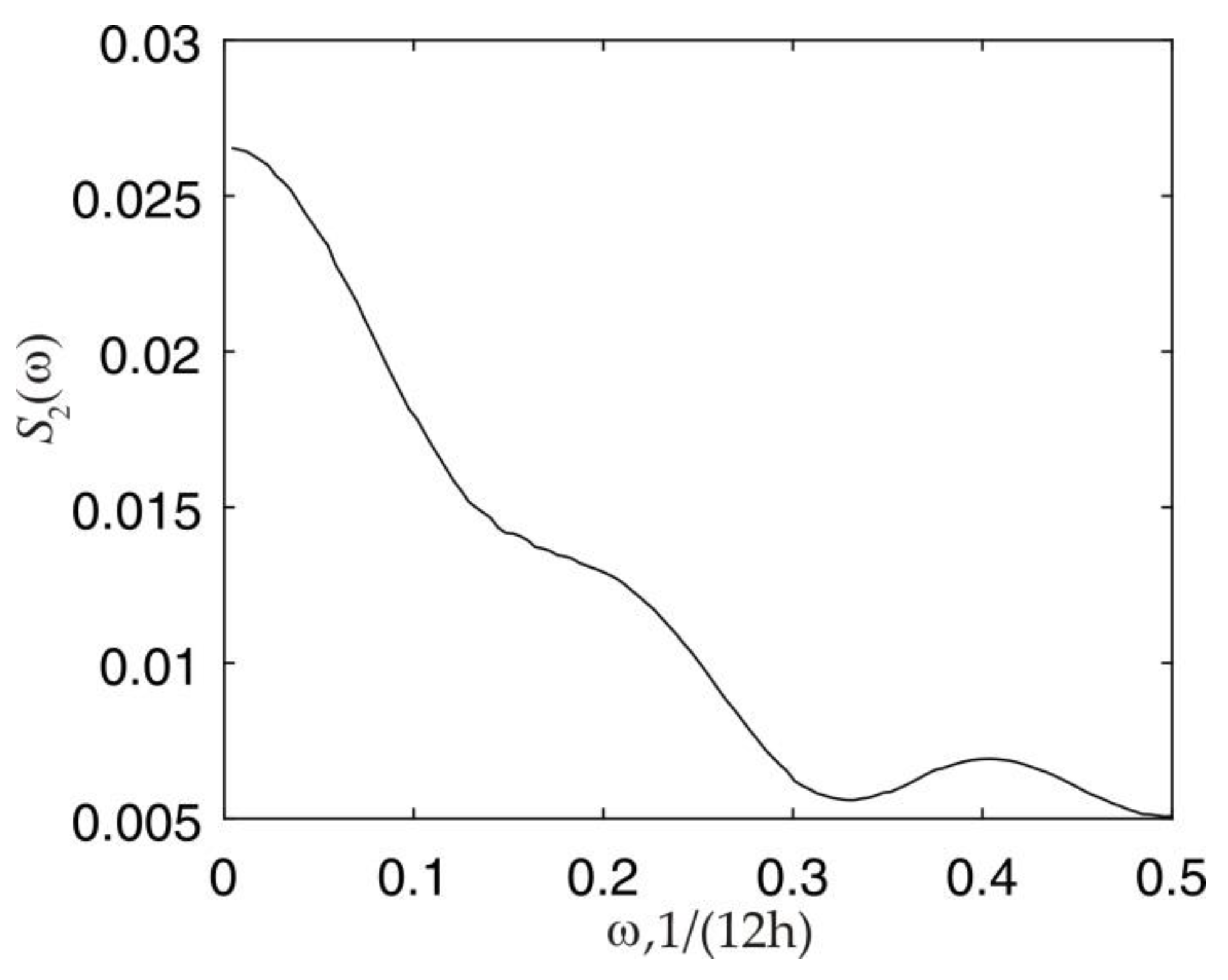
In Figure 6, which shows the spectral density for the e_{t, 2} errors, the sample spectrum of this time series resembles the spectrum of a first-order autoregressive process [15,16,17]. However, we note that the stochastic process is not uniquely determined by its spectral density [8]. Therefore, as previously mentioned, we need to include two additional constraints that the resulting model be invertible and realizable. This will ensure that we have a unique model.

Based on the theoretical properties of the process, the error models are

e_t,1 − η₁₁e_{(t−1), 1} − η₂₁e_{(t−2), 1} − η₃₁e_{(t−3), 1} = ε_{t, 1}
e_{t, 2} − η₁₂e_{(t−1), 2} = ε_{t, 2}

(21)

e_t,3 − η₁₃e_{(t−1), 3} − η₂₃e_{(t−2), 3} − η₃₃e_{(t−3), 3} = ε_{t, 3}

where η are the parameters to be determined. These parameters can be found using the approach presented in Section 2.2 by multiplying the finite impulse response model by the delayed errors and taking the expectations. For example, for e₁, this gives

γ_i = η₁₁γ_i−1 + η₂₁γ_i−2 + η₃₁γ_i−3, i = 1, 2, 3

(22)

where γ_i = cov(e_t1, e_(t−i)1) = γ_−i.

For the process e_{t, 1}, the estimates of the coefficients η₁₁, η₂₁ and η₃₁ are, respectively, equal to 0.4131, −0.0093, and −0.0528. These values were used as the initial guesses passed to the PEM function. As a result of calculations, the model parameters were found to be: η₁₁ = 0.4175, η₂₁ = 0.03234, η₃₁ = −0.07026. The initial value of coefficient η₁₂ is 0.3748 and its final value is η₁₂ = 0.3758.

Similarly, using Equation (22), the initial guesses were η₁₃ = 0.5142, η₂₃ = −0.0507, and η₃₃ = −0.0207 to give final values of η₁₃ = 0.5151, η₂₃ = −0.02676, and η₃₃ = −0.03246.

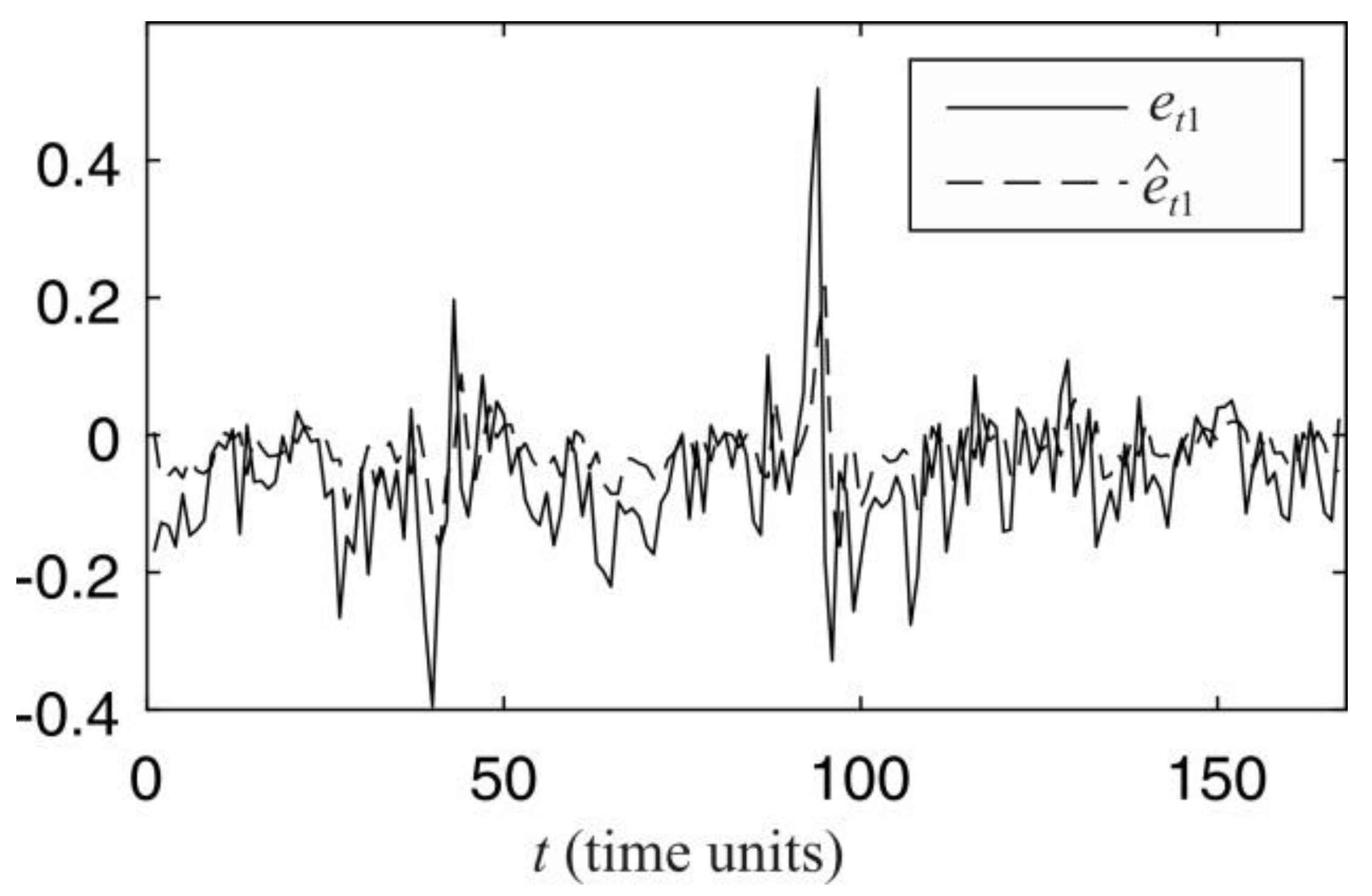
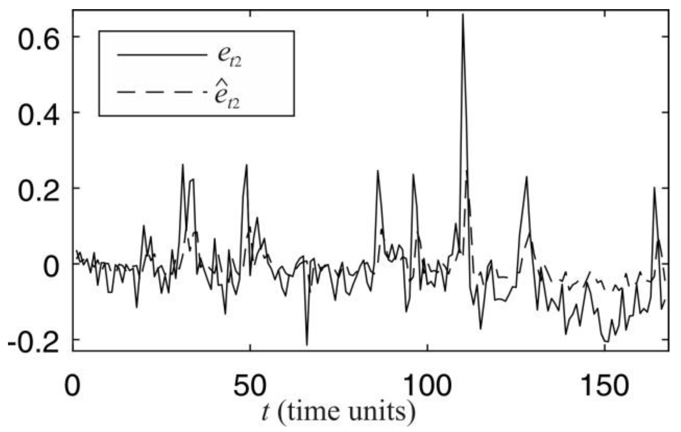
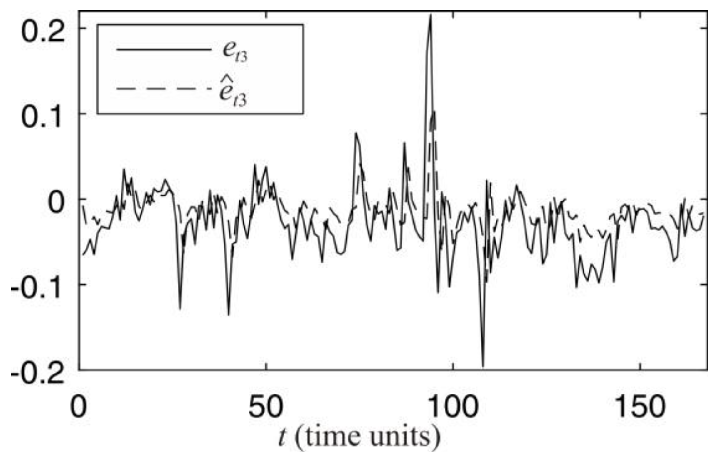
The performance of predictive filter models obtained from the analysis of the training dataset is validated using the testing sample. Figure 7, Figure 8 and Figure 9 compare the predictions against the true values, where the solid line shows the true e_{t, m} errors and the dashed line their predicted values for m = 1, 2, and 3. At the time point t on the x-axis, the corresponding error e_{t, m} and the predicted error ${\widehat{e}}_{t,m}$ computed at t − 1.

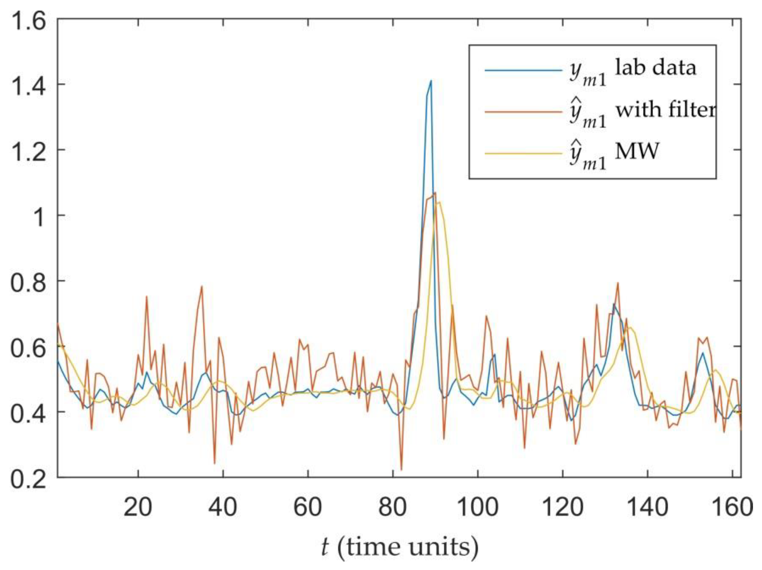
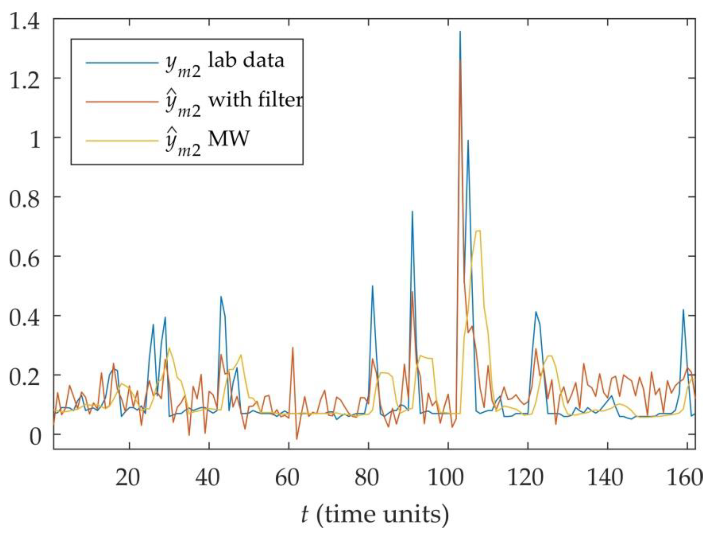
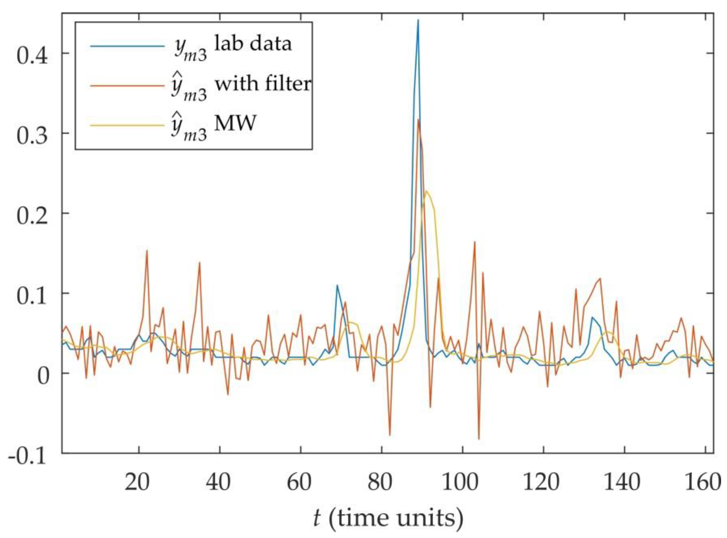
Figure 10, Figure 11 and Figure 12 compare the performance of the soft sensors with the proposed filter for error prediction and a traditional method, in which adaptive bias term is calculated based on the moving window (MW) approach [18]. It can be seen that the filter provides better tracking of the process values, therefore improving the accuracy of the overall soft sensor system reducing the MSE of the output variables y₁, y₂, and y₃ by 32%, 67%, and 9.5%, respectively.

4. Conclusions

This paper proposed a new approach to handling the bias update term in a soft sensor system. Rather than purely using available samples, the new bias update term seeks to predict what the errors will be in the future. Tests of this approach on a reactive distillation column show that the approach can handle the errors well. However, the predictive filters used only work for areas without serious disturbances or outliers.

Therefore, it makes sense to consider more complex models for the predictive filters including models with an additional component in the form of some flow, for example, Poissonian flow, of events (outliers). If the flow of outliers is added to the process model then the intensity of this flow needs to be estimated. In this case, the number of outliers in the training dataset should be sufficient to estimate the intensity of the flow of outliers with acceptable accuracy.