Green’s Function Related to a n-th Order Linear Differential Equation Coupled to Arbitrary Linear Non-Local Boundary Conditions

Abstract

In this paper, we obtain the explicit expression of the Green’s function related to a general n-th order differential equation coupled to non-local linear boundary conditions. In such boundary conditions, an n dimensional parameter dependence is also assumed. Moreover, some comparison principles are obtained. The explicit expression depends on the value of the Green’s function related to the two-point homogeneous problem; that is, we are assuming that when all the parameters involved on the boundary conditions take the value zero then the problem has a unique solution, which is characterized by the corresponding Green’s function g. The expression of the Green’s function G of the general problem is given as a function of g and the real parameters considered at the boundary conditions. It is important to note that, in order to ensure the uniqueness of the solution of the considered linear problem, we must assume a non-resonant additional condition on the considered problem, which depends on the non-local conditions and the corresponding parameters. We point out that the assumption of the uniqueness of the solution of the two-point homogeneous problem is not a necessary condition to ensure the existence of the solution of the general case. Of course, in this situation, the expression we are looking for must be obtained in a different manner. To show the applicability of the obtained results, a particular example is given.

1. Introduction

Most of the real phenomena that appear in fields such as physics, engineering, biology or medicine are modeled by ordinary differential equations coupled with suitable boundary conditions located at some given set of the interval of definition. The majority of them take values at the extremes of the interval, and they are known as two-point boundary value problems. There is a long tradition in studying these kinds of problems, and a lot of works in this direction have been developed to ensure the existence, uniqueness or multiplicity of solutions, as well as their stability or instability (see, for instance, [1,2]).

Allowing, on the boundary conditions, suitable dependence at some fixed points (or sets) of the interval that are not the extreme ones permits the study of a wider set of problems that model suitable real phenomena. Therefore, the so-called non-local conditions allow us to deal with more complicated problems that model more difficult real phenomena. In the non-resonant case, such kinds of problems can be studied as an equivalent integral equation of the type

$$u\left(t\right)=r\left(t\right)B\left(u\right)+{\int }_a^{b}k(t,s)f(s,u\left(s\right))ds,t\in [a,b],$$

where r is a continuous function, $B:C\left(\right[a,b\left]\right)\to \mathbb{R}$ is a continuous linear functional, k is the Green’s function related to the considered problem, and f is the non-linear part of the considered equation.

This kind of equation covers different non-local situations as, for instance, modeling the steady-state of a heated bar of length $b-a$ subject to a thermostat, where a controller in one end adds or removes heat accordingly to the temperature measured by a sensor located at a certain point of the bar. This type of heat-flow problem has been studied in several works on the literature; see [3,4,5,6] and references therein. These types of problems are known as multipoint boundary value problems. The Green’s function for this situation is obtained in some references; see, for instance, [7]. The multipoint conditions also appear in a natural way when we are studying the behavior of a bridge that has several pillars. Such behavior is modeled by a fourth-order equation, see [8] and references therein, defined in an interval $[a,b]$. The points $x=a$ and $x=b$ are the extremes of the bridge. Thus, assuming that the pillars of the bridge are located at the points $a<a_1<\cdots <a_m<b$, it is expected that there is a relationship between the position of the bridge at the ends and at the pillars. Therefore, the multipoint conditions could be written as

$$u^{\left(j\right)}\left(a\right)=\sum _{i=1}^m{\alpha }_i^{j}u\left(a_i\right),u^{\left(j\right)}\left(b\right)=\sum _{i=1}^m{\beta }_i^{j}u\left(a_i\right),j=0,\dots ,n-1,$$

with ${\alpha }_i^j{\beta }_i^j$, $i=1,\dots ,m$, $j=0,\dots ,n-1$, given real constants.

Of course, there are more situations to deal with, and several combinations of the multipoint boundary conditions could be considered. It is important to point out that to maintain the structure of the bridge as stable, it is essential that the movement of the bridge occurs in the same direction of the force to which it is subjected. As it can be seen in [9], this property is equivalent to the fact that the related Green’s function has a constant sign. For this reason, the construction of the Green’s function as well as the study of its sign will be essential.

An important part of the methods used to ensure the existence of solutions is mainly related to the theory of lower and upper solutions [2], degree theory [4,5,10] or monotone iterative techniques [9]. In all of these cases, it is fundamental to ensure the constant sign (in the whole square of definition or in a suitable subset) of the Green’s function related to the considered problem. In many situations, this study is not trivial and requires many tedious and complicated calculations. Such difficulty increases with non-local operators on the boundary. Some of the most common non-local boundary conditions are given as integral equations (some of them in the Stieltjes sense) and have been applied to different situations as fourth-order beam equations [11], second-order problems [12] or fractional equations [13,14]. The concept of generalized Green’s function appears in the resonance case and also on partial differential equations. For such problems, the methods from the monographs [15,16] can be used.

To be concise, in this paper, we will consider the following n-th order linear boundary value problem with parameter dependence:

$$\left\{\begin{array}{cccc}\hfill T_n\left[M\right]u\left(t\right)& =\hfill & \sigma \left(t\right),\hfill & t\in I:=\left[a,b\right],\hfill \\ \hfill B_i\left(u\right)& =\hfill & {\delta }_i{C}_i\left(u\right),\hfill & i=1,\dots ,n,\hfill \end{array}\right.$$

(1)

where

$$T_n\left[M\right]u\left(t\right):=L_{n}u\left(t\right)+Mu\left(t\right),t\in I,$$

with

$$L_{n}u\left(t\right):=u^{\left(n\right)}\left(t\right)+a_1\left(t\right)u^{\left(n-1\right)}\left(t\right)+\cdots +a_n\left(t\right)u\left(t\right),t\in I.$$

Here, $\sigma$ and $a_k$ are continuous functions for all $k=0,\dots ,n-1$, $M\in \mathbb{R}$ and ${\delta }_i\in \mathbb{R}$ for all $i=1,\dots ,n$.

Moreover, $C_i:C\left(I\right)\to \mathbb{R}$ is a linear continuous operator and $B_i$ covers the general two-point linear boundary conditions, i.e.:

$${\displaystyle B_i\left(u\right)=\sum _{j=0}^{n-1}\left({\alpha }_j^i{u}^{\left(j\right)}\left(a\right)+{\beta }_j^i{u}^{\left(j\right)}\left(b\right)\right),i=1,\dots ,n,}$$

where ${\alpha }_j^i,{\beta }_j^i$ real constants for all $i=1,\dots ,n,j=0,\dots ,n-1$.

Remark 1.

Examples of operator $C_i$ can be the integral operator

$${\displaystyle C_i\left(u\right)={\int }_{J}u\left(s\right)v\left(s\right)ds,J\subset I(J an interval)}\mathrm{with}v\in C\left(J\right),$$

or the multipoint operator

$${\displaystyle C_i\left(u\right)=\sum _{k=1}^r{ϵ}_{k}u\left({\nu }_k\right),{\nu }_k\in I,{ϵ}_k\in \mathbb{R},k=0,\dots ,r.}$$

We point out that Problem (1) covers any n-th order differential equation and that on the choice of ${\delta }_i$, any of them could vanish, so it may be thought as a perturbation of a two-point boundary value problem.

Therefore, by considering the following homogeneous problem related to the general Equation (1):

$$\left\{\begin{array}{cc}\hfill T_n\left[M\right]u\left(t\right)& =0,t\in I,\hfill \\ \hfill B_i\left(u\right)& =0,i=1,\dots n,\hfill \end{array}\right.$$

(2)

we will obtain the explicit expression of the Green’s function related to the non-local problem (1) under the assumption that the corresponding homogeneous Problem (2) has only the trivial solution. Moreover, we will characterize the spectrum of Problem (1) as a function of the value of the non-local operators over functions related to the Green’s function of Problem (1).

We notice that the non-local linear operators depend only on the values of the function that we are looking for, but in a more general framework, they could depend on any of its derivatives, and by using analogous reasoning, the result that we could obtain would be similar.

The paper is organized as follows. In the next section, we obtain the expression of the Green’s function related to Problem (1) and characterize its spectrum. In Section 3, we present an example where the formula is used to obtain the corresponding expression and to describe the exact set of parameters for which its Green’s function has a constant sign on $I\times I$.

2. Explicit Expression of the Solution of Problem (1)

This section is devoted to deduce the explicit expression of the solution of the general Problem (1). To this end, we assume that the homogeneous Problem (2) has as a unique solution the trivial one. In such a case, it is very well known that Problem (1), with ${\delta }_i=0$, $i=0,\dots ,n$, has a unique solution for any $\sigma \in C\left(I\right)$ given. Moreover, such solution is given by

$${\displaystyle v\left(t\right)={\int }_a^b{g}_M\left(t,s\right)\sigma \left(s\right)ds.}$$

(3)

Here, $g_M$ denotes the Green’s function related to Problem (2), which exists and is unique (see, for details, [9,17]).

Now, we formulate the following particular case of the result proved in ([9], page 35):

Theorem 1.

The boundary value problem

$$T_n\left[M\right]u\left(t\right)=\sigma \left(t\right),t\in I,B_i\left(u\right)=h_i,i=1,\dots ,n,$$

(4)

has a unique solution for any $\sigma \in C\left(I\right)$ and $h_i\in \mathbb{R}$, $i\in \{0,1,\dots ,n\}$, if and only if

$$det\left(\begin{array}{ccc}{B}_1\left(u_1\right)& \dots & B_1\left(u_n\right)\\ ⋮& \ddots & ⋮\\ B_n\left(u_1\right)& \dots & B_n\left(u_n\right)\end{array}\right)\ne 0,$$

(5)

where $\left(u_1,\dots ,u_n\right)$ is any set of linearly independent solutions of $T_n\left[M\right]u\left(t\right)=0$.

Remark 2.

It is immediate to verify that the fact that the determinant in the previous result is different from zero does not depend on the chosen set of linearly independent solutions.

Remark 3.

Notice that condition (5) is independent of the nonhomogeneous part of Problem (4): σ and $h_i$, $i\in \{1,\dots ,n\}$.

Remark 4.

One can see in ([9], page 35) that the following property

$$\mathrm{rank}\left(\begin{array}{ccc}{\alpha }_0^1& \dots & {\alpha }_{n-1}^1\\ ⋮& \ddots & ⋮\\ {\alpha }_0^n& \dots & {\alpha }_{n-1}^n\end{array}|\begin{array}{ccc}{\beta }_0^1& \dots & {\beta }_{n-1}^1\\ ⋮& \ddots & ⋮\\ {\beta }_0^n& \dots & {\beta }_{n-1}^n\end{array}\right)=n,$$

(6)

is a necessary (but not sufficient) condition to ensure the uniqueness of the solution of Problem (4).

As a direct consequence of Theorem 1, we deduce the following result.

Lemma 1.

There exists a unique Green’s function related to Problem (2), $g_M$, if and only if for any $i\in \{1,\cdots ,n\}$, the following problem

$$\left\{\begin{array}{cc}\hfill T_n\left[M\right]u\left(t\right)& =0,t\in I,\hfill \\ \hfill B_j\left(u\right)& =0,j\ne i,\hfill \\ \hfill B_i\left(u\right)& =1,\hfill \end{array}\right.$$

(7)

has a unique solution, which we denote as ${\omega }_i\left(t\right)$, $t\in I$.

In the following result, under suitable assumptions concerning the spectrum of the considered problem, we prove the existence and uniqueness of the solution of Problem (1). Moreover, the expression of its related Green’s function is obtained.

Theorem 2.

Assume that Problem (2) has $u=0$ as its unique solution and let $g_M$ be its related Green’s function. Let $\sigma \in C\left(I\right)$, and ${\delta }_i,$$i=1,\cdots ,n$, be such that

$$det(I_n-A)\ne 0,$$

(8)

with $I_n$, the identity matrix of order n and $A={\left(a_{ij}\right)}_{n\times n}\in {\mathcal{M}}_{n\times n}$ given by

$$a_{ij}={\delta }_j{C}_i\left({\omega }_j\right),i,j\in \{1,\dots ,n\}.$$

Then, Problem (1) has a unique solution $u\in C^n\left(I\right)$, given by the expression

$${\displaystyle u\left(t\right)={\int }_a^{b}G\left(t,s,{\delta }_1,\dots ,{\delta }_n,M\right)\sigma \left(s\right)ds,}$$

(9)

where

$$G\left(t,s,{\delta }_1,\dots ,{\delta }_n,M\right):=g_M\left(t,s\right)+\sum _{i=1}^n\sum _{j=1}^n{\delta }_i{b}_{ij}{\omega }_i\left(t\right)C_j\left(g_M(·,s)\right),t,s\in I,$$

(10)

with ${\omega }_j$ defined on Lemma 1 and $B={\left(b_{ij}\right)}_{n\times n}={(I_n-A)}^{-1}$.

Proof. 

Since Problem (1) has a unique solution when ${\delta }_i=0$ for all $i=1,\dots ,n$, from Lemma 1 we know that any solution of (1) satisfies the following expression

$${\displaystyle u\left(t\right)=v\left(t\right)+\sum _{i=1}^n{\omega }_i\left(t\right){\delta }_i{C}_i\left(u\right),t\in I,}$$

(11)

with v given by (3).

Applying linear continuous operators $C_j$ on both sides of (11), we infer that

$${\displaystyle C_j\left(u\right)=C_j\left(v\right)+C_j\left({\displaystyle \sum _{i=1}^n{\delta }_i{\omega }_{i}C\left(u\right)}\right)=C_j\left(v\right)+\sum _{i=1}^n{\delta }_i{C}_j\left({\omega }_i\right)C_i\left(u\right),j=1,\cdots ,n,}$$

from which we deduce that

$$\begin{array}{c}\hfill C_j\left(u\right)-\sum _{i=1}^n{\delta }_i{C}_j\left({\omega }_i\right)C_i\left(u\right)=C_j\left(v\right),j=1,\cdots ,n.\end{array}$$

Therefore, we arrive at the following system of equations

$$(I_n-A)\left(\begin{array}{c}{C}_1\left(u\right)\\ C_2\left(u\right)\\ ⋮\\ C_n\left(u\right)\end{array}\right)=\left(\begin{array}{c}{C}_1\left(v\right)\\ C_2\left(v\right)\\ ⋮\\ C_n\left(v\right)\end{array}\right).$$

(12)

From the previous equality, we deduce that

$$C_i\left(u\right)=\sum _{j=1}^n{b}_{ij}{C}_j\left(v\right),i=1,\cdots ,n,$$

and substituting this expression in (11), we obtain that

$$u\left(t\right)=v\left(t\right)+\sum _{i=1}^n{\delta }_i{\omega }_i\left(t\right)\left(\sum _{j=1}^n{b}_{ij}{C}_j\left(v\right)\right),t\in I.$$

To calculate $C_j\left(v\right)$, we use the fact that $C_j$ is linear and continuous, so we obtain that

$${\displaystyle C_j\left(v\right)=C_j\left({\displaystyle {\int }_a^b{g}_M\left(·,s\right)\sigma \left(s\right)ds}\right)={\int }_a^b{C}_j\left(g_M\left(·,s\right)\right)\sigma \left(s\right)ds.}$$

Using the previous equality, we have that

$$\begin{array}{cc}\hfill u\left(t\right)& {\displaystyle ={\int }_a^b{g}_M\left(t,s\right)\sigma \left(s\right)ds+\sum _{i=1}^n{\delta }_i{\omega }_i\left(t\right)\left(\sum _{j=1}^n{b}_{ij}{\int }_a^b{C}_j\left(g_M\left(·,s\right)\right)\sigma \left(s\right)ds\right)}\hfill \\ \hfill & {\displaystyle ={\int }_a^b\left(g_M\left(t,s\right)+\sum _{i=1}^n{\delta }_i{\omega }_i\left(t\right)\left(\sum _{j=1}^n{b}_{ij}{C}_j\left(g_M(·,s)\right)\right)\right)\sigma \left(s\right)ds}\hfill \\ \hfill & {\displaystyle ={\int }_a^b\left(g_M\left(t,s\right)+\sum _{i=1}^n\sum _{j=1}^n{\delta }_i{b}_{ij}{\omega }_i\left(t\right)C_j\left(g_M(·,s)\right)\right)\sigma \left(s\right)ds}\hfill \\ \hfill & {\displaystyle ={\int }_a^{b}G\left(t,s,{\delta }_1,\dots ,{\delta }_n,M\right)\sigma \left(s\right)ds.}\hfill \end{array}$$

Therefore, we have proved that under assumption (8) in conjunction with the uniqueness of the solution of Problem (2), Problem (1) has at least one solution given by expression (9).

To conclude the proof, we must show the uniqueness of solution. To this end, suppose that u and v are two different solutions of Problem (1). Then,

$$\left\{\begin{array}{cccc}\hfill T_n\left[M\right]\left(u-v\right)\left(t\right)& =\hfill & 0,\hfill & t\in I,\hfill \\ \hfill B_i\left(u-v\right)& =\hfill & {\delta }_i{C}_i\left(u-v\right),\hfill & i=1,\dots ,n.\hfill \end{array}\right.$$

(13)

As a consequence, we have that

$${\displaystyle \left(u-v\right)\left(t\right)=\sum _{i=1}^n{\delta }_i{C}_i\left(u-v\right){\omega }_i\left(t\right),t\in I.}$$

Applying operator $C_j$ on both sides again, we have that

$${\displaystyle C_j\left(u-v\right)=\sum _{i=1}^n{\delta }_i{C}_i\left(u-v\right)C_j\left({\omega }_i\right),j=1,\cdots ,n,}$$

or, which is the same,

$$(I_n-A)\left(\begin{array}{c}{C}_1(u-v)\\ C_2(u-v)\\ ⋮\\ C_n(u-v)\end{array}\right)=\left(\begin{array}{c}0\\ 0\\ ⋮\\ 0\end{array}\right).$$

Condition (8) implies that $C_i\left(u-v\right)=0$ for $i=1,\cdots ,n$. Hence, from (13), we deduce that $u-v$ is a solution of the homogeneous problem

$$\left\{\begin{array}{cc}\hfill T_n\left[M\right]\left(u-v\right)\left(t\right)& =0,t\in I,\hfill \\ \hfill B_i\left(u-v\right)& =0,i=1,\dots ,n.\hfill \end{array}\right.$$

Since this problem has only the trivial solution, we deduce that $u=v$ on I, and the proof is concluded. □

Remark 5.

We notice that in the previous result, we assume that there is a unique Green’s function related to Problem (2). Such condition does not depend on ${\delta }_i$ or operators $C_i$, $i=1,\dots ,n$. It is obvious that this condition is fundamental to construct function G on (10). However, such condition is not necessary in order to deduce the existence and uniqueness of the solution of Problem (1). In a practical situation, our hypotheses ensure the existence of a unique solution of Problem (1) provided for any parameters $(M,{\delta }_1,\dots ,{\delta }_n)$, such that M is not an eigenvalue of Problem (2). However, as we will see in the next section, this condition is not necessary, and Problem (2) could have a unique solution for some choice of $(M,{\delta }_1,\dots ,{\delta }_n)$, with M an eigenvalue of Problem (2).

Moreover, we assume the non-spectral condition (8), which is equivalent to assume that 1 is not an eigenvalue of matrix A. When such condition fails, we have that Problem (1) does not have a unique solution. Therefore, this non-spectral condition characterizes the uniqueness of the solution of Problem (1) provided the existence of $g_M$ is assumed. In the case of M being an eigenvalue of Problem (2), condition (8) makes no sense because ${\omega }_i$ does not exist.

We also notice that obtaining the explicit expression of the Green’s function $g_M$ (for the non-local case ${\delta }_i=0$, $i=1,\dots ,n$) is not an easy problem. In fact, when the coefficients of operator $L_n$ are not constant, such expression would be given, in the majority of the situations, as a series expansion of the eigenfunctions of the considered homogeneous problem, see [17,18,19] and references therein. We point out that in [20], an algorithm has been developed that calculates the exact expression of the Green’s function related to any n-th order differential equation, with constant coefficients coupled with arbitrary two-point linear boundary conditions. Such algorithm has been developed in a Mathematica package, and it is available at [21].

We will analyze now the particular case of considering that all the functionals at the boundary conditions are the same (that is, there is some linear continuous operator C such that $C_i=C$ for $i=1,\cdots ,n$). In this case, since we have only $C\left(u\right)$ as a unique unknown variable, system (12) reduces to the one-dimensional equation

$$\left(1-\sum _{i=1}^n{\delta }_{i}C\left({\omega }_i\right)\right)C\left(u\right)=C\left(v\right),$$

(14)

and condition (8) reduces to

$$\sum _{i=1}^n{\delta }_{i}C\left({\omega }_i\right)\ne 1.$$

(15)

Therefore, it is obvious that

$$C\left(u\right)=\frac{C\left(v\right)}{{\displaystyle 1-\sum _{i=1}^n{\delta }_{i}C\left({\omega }_i\right)}}.$$

(16)

As a direct consequence, we obtain the following result for this particular case.

Corollary 1.

Assume that Problem (2) has $u=0$ as its unique solution and let $g_M$ be its unique Green’s function. Let $\sigma \in C\left(I\right)$, and ${\delta }_i,$$i=1,\cdots ,n$, be such that (15) holds. Then, problem

$$\left\{\begin{array}{cccc}\hfill T_n\left[M\right]u\left(t\right)& =\hfill & \sigma \left(t\right),\hfill & t\in I,\hfill \\ \hfill B_i\left(u\right)& =\hfill & {\delta }_{i}C\left(u\right),\hfill & i=1,\dots ,n,\hfill \end{array}\right.$$

(17)

has a unique solution $u\in C^n\left(I\right)$, given by the expression

$${\displaystyle u\left(t\right)={\int }_a^{b}G\left(t,s,{\delta }_1,\dots ,{\delta }_n,M\right)\sigma \left(s\right)ds,}$$

where

$$G\left(t,s,{\delta }_1,\dots ,{\delta }_n,M\right):=g_M\left(t,s\right)+{\displaystyle \frac{{\displaystyle \sum _{i=1}^n{\delta }_i{\omega }_i\left(t\right)}}{{\displaystyle 1-\sum _{j=1}^n{\delta }_{j}C\left({\omega }_j\right)}}}C\left(g_M\left(·,s\right)\right).$$

(18)

Proof. 

It is enough to show that, in this case, expression (10) can be rewritten as (18).

Indeed, since we have a unique functional C (and so, the sum in j reduces to a unique term), it is clear that we can argue as in the proof of Theorem 2, by denoting

$$I_n-A\equiv \left(a_{11}\right)=\left({\displaystyle 1-\sum _{i=1}^n{\delta }_{i}C\left({\omega }_i\right)}\right)$$

and

$$B={(I_n-A)}^{-1}\equiv \left(b_{11}\right)=\left(\frac{1}{{\displaystyle 1-\sum _{i=1}^n{\delta }_{i}C\left({\omega }_i\right)}}\right).$$

As a consequence, we deduce that expression (10) is rewritten in this case as

$$\begin{array}{cc}\hfill G\left(t,s,{\delta }_1,\dots ,{\delta }_n,M\right)& =g_M\left(t,s\right)+\sum _{i=1}^n{\delta }_i{b}_{11}{\omega }_i\left(t\right)C\left(g_M(·,s)\right)\hfill \\ \hfill & =g_M\left(t,s\right)+{\displaystyle \frac{{\displaystyle \sum _{i=1}^n{\delta }_i{\omega }_i\left(t\right)}}{{\displaystyle 1-\sum _{j=1}^n{\delta }_{j}C\left({\omega }_j\right)}}}C\left(g_M\left(·,s\right)\right).\hfill \end{array}$$

□

Example 1.

If operator C is given by ${\displaystyle C\left(u\right)={\int }_a^{b}u\left(s\right)ds}$, then

$$\begin{array}{cc}\hfill C\left({\displaystyle {\int }_a^b{g}_M\left(t,s\right)\sigma \left(s\right)ds}\right)& {\displaystyle ={\int }_a^b\left({\displaystyle {\int }_a^b{g}_M\left(t,s\right)\sigma \left(s\right)ds}\right)dt}\hfill \\ \hfill & {\displaystyle ={\int }_a^b\left({\displaystyle {\int }_a^b{g}_M\left(t,s\right)dt}\right)\sigma \left(s\right)ds={\int }_a^{b}C\left(g_M\left(·,s\right)\right)\sigma \left(s\right)ds.}\hfill \end{array}$$

Example 2.

If C is defined as $C\left(u\right)=u\left(c\right)$, for some $c\in (a,b)$, we have that

$$\begin{array}{cc}\hfill C\left({\displaystyle {\int }_a^b{g}_M\left(t,s\right)\sigma \left(s\right)ds}\right)& {\displaystyle ={\int }_a^b{g}_M\left(c,s\right)\sigma \left(s\right)ds={\int }_a^{b}C\left(g_M\left(·,s\right)\right)\sigma \left(s\right)ds.}\hfill \end{array}$$

As a direct consequence of expression (18), we deduce the following comparison result:

Corollary 2.

Assume that Problem (2) has $u=0$ as its unique solution and let $g_M$ be its unique Green’s function. Assume that condition (15) holds and let G be the Green’s function related to Problem (17). Suppose that the following hypotheses are satisfied:

(a) 

${\displaystyle \sum _{j=1}^n{\delta }_{j}C\left({\omega }_j\right) <1}$.

(b) 

${\delta }_i{\omega }_i\left(t\right) \ge 0$, $\forall t\in I,i=1,\cdots ,n$.

(c) 

If $u\ge 0$ on I, then $C\left(u\right) \ge 0$.

Then, the following assertions are fulfilled:

(i) 

If $g_M\left(t,s\right) \ge 0$, for all $\left(t,s\right)$ on $I\times I$ then $G\left(t,s,{\delta }_1,\dots ,{\delta }_n,M\right) \ge g_M\left(t,s\right) \ge 0$ for all $\left(t,s\right)$ on $I\times I$.

(ii) 

If $g_M\left(t,s\right) \le 0$, for all $\left(t,s\right)$ on $I\times I$ then $G\left(t,s,{\delta }_1,\dots ,{\delta }_n,M\right) \le g_M\left(t,s\right) \le 0$ for all $\left(t,s\right)$ on $I\times I$.

Remark 6.

As we will see in the next section, the conditions of the previous corollary are sufficient but not necessary to ensure the positiveness of the related Green’s function.

Now, considering $M\in \mathbb{R}$ and ${\delta }_j,j\ne k$ fixed, by differentiating equality (18) with respect to ${\delta }_k$ we deduce that

$${\displaystyle \frac{\partial G}{\partial {\delta }_k}}\left(t,s,{\delta }_1,{\delta }_2,\cdots ,{\delta }_n,M\right)={\displaystyle \frac{{\displaystyle {\omega }_k\left(t\right)\left({\displaystyle 1-\sum _{j=1}^n{\delta }_{j}C\left({\omega }_j\right)}\right)+C\left({\omega }_k\right)\sum _{j=1}^n{\delta }_j{\omega }_j\left(t\right)}}{{\left({\displaystyle 1-\sum _{j=1}^n{\delta }_{j}C\left({\omega }_j\right)}\right)}^2}}C\left(g_M\left(·,s\right)\right).$$

(19)

Thus, we can study the monotony of the Green’s function related to Problem (17) with respect to any parameter ${\delta }_k$.

3. First Order Periodic Problem

This section is devoted to showing the applicability of the expression (18) obtained in the previous section. Moreover, we show the validity of the assumptions of Theorem 2 and Corollary 2.

To be concise, we study the sign of the Green’s function related to the following perturbed first-order periodic problem.

$$\left\{\begin{array}{cccc}\hfill u^{\prime }\left(t\right)+Mu\left(t\right)& =\hfill & \sigma \left(t\right),\hfill & t\in \left[0,1\right],\hfill \\ \hfill u\left(0\right)-u\left(1\right)& =\hfill & {\displaystyle \delta {\int }_0^{1}u\left(s\right)ds,}\hfill \end{array}\right.$$

(20)

with $M,\delta \in \mathbb{R}$.

It is immediate to verify that the spectrum of Problem (20) is given by

$${\Lambda }_{M\delta }=\{\left(M,\delta \right)\in {\mathbb{R}}^2,M=\delta \}.$$

In particular, when we consider the homogeneous periodic problem ($\delta =0$):

$$\left\{\begin{array}{cc}\hfill u^{\prime }\left(t\right)+Mu\left(t\right)& =\sigma \left(t\right),t\in \left[0,1\right],\hfill \\ \hfill u\left(0\right)-u\left(1\right)& =0,\hfill \end{array}\right.$$

(21)

we have that $M=0$ is the unique eigenvalue of the considered problem. That is, there is a unique $g_M$ if and only if $M\ne 0$. Moreover, see [9], it is immediate to verify that the expression of the Green’s function of Problem (21) is given by

$$g_M\left(t,s\right)=\frac{1}{1-e^{-M}}\left\{\begin{array}{cc}{e}^{-M\left(t-s\right)},\hfill & 0\le s\le t\le 1,\hfill \\ e^{-M\left(t-s+1\right)},\hfill & 0<t<s\le 1.\hfill \end{array}\right.$$

(22)

Using the notations of Lemma 1, it is not difficult to verify, see [9], that

$${\omega }_1\left(t\right)=g_M\left(t,0\right)=\frac{e^{-Mt}}{1-e^{-M}},t\in I.$$

As a consequence, in this case, condition (15) is written as $\delta \ne M$, $M\ne 0$. Thus, Formula (18) can be applied to this set of $(M,\delta )$. We point out that, in this case, it is valid for all the values $\left(M,\delta \right)$ that are not on the spectrum of (20) except the ones given by $(0,\delta )$, with $\delta \ne 0$. The expression for this last situation must be studied separately.

First, we deduce the following symmetry property of the Green’s function related to Problem (20).

Lemma 2.

Assume that Problem (20) has a unique solution and let $G\left(t,s,\delta ,M\right)$ be its related Green’s function. Then, the following symmetry property holds:

$$G\left(t,s,\delta ,M\right) =-G\left(1-t,1-s,-\delta ,-M\right).$$

(23)

Proof. 

Let

$$u\left(t\right)={\int }_0^{1}G\left(t,s,\delta ,M\right)\sigma \left(s\right)ds$$

be the unique solution of Problem (20).

It is immediate to verify that $v\left(t\right):=u(1-t)$ is the unique solution of the following problem:

$$\left\{\begin{array}{cccc}\hfill v^{\prime }\left(t\right)-Mv\left(t\right)& =\hfill & -\sigma \left(1-t\right),\hfill & t\in \left[0,1\right],\hfill \\ \hfill v\left(0\right)-v\left(1\right)& =\hfill & {\displaystyle -\delta {\int }_0^{1}v\left(s\right)ds.}\hfill \end{array}\right.$$

As a direct consequence, we deduce that

$$v\left(t\right)=-{\int }_0^{1}G\left(t,s,-\delta ,-M\right)\sigma (1-s)ds.$$

On the other hand, we have

$$v\left(t\right)=u(1-t)={\int }_0^{1}G\left(1-t,s,\delta ,M\right)\sigma \left(s\right)ds={\int }_0^{1}G\left(1-t,1-s,\delta ,M\right)\sigma (1-s)ds.$$

Therefore, the equality (23) is fulfilled directly by identifying the two previous equalities. □

Therefore, it is enough to study the sign of the Green’s function $G\left(t,s,\delta ,M\right)$ for $M>0$ and $\delta \ne M$ (the case $M=0$ and $\delta \ne 0$ will be considered further).

In our case, the expression (18) is given by the following formula:

$${\displaystyle G\left(t,s,\delta ,M\right) =g_M\left(t,s\right)+{\displaystyle \frac{\delta g_M\left(t,0\right)}{{\displaystyle 1-\delta {\int }_0^1{g}_M\left(t,0\right)dt}}}{\int }_0^1{g}_M\left(t,s\right)dt.}$$

One can easily verify that

$$C\left(g_M(·,s)\right):={\int }_0^1{g}_M\left(t,s\right)dt=\frac{1}{M}\mathrm{for} \mathrm{all} s\in \left[0,1\right] \mathrm{and} M\ne 0.$$

Thus, we arrive at the following explicit expression of the Green’s function G:

$$G\left(t,s,\delta ,M\right) =\frac{\delta }{M-\delta }{\displaystyle \frac{e^{-Mt}}{1-e^{-M}}}+\frac{1}{1-e^{-M}}\left\{\begin{array}{cc}{\displaystyle e^{-M\left(t-s\right)},}\hfill & 0\le s\le t\le 1,\hfill \\ {\displaystyle e^{-M\left(t-s+1\right)},}\hfill & 0<t<s\le 1.\hfill \end{array}\right.$$

(24)

Remark 7.

We point out that, since for all $s\in (0,1)$, it is verified that

$$\underset{t\to s^{+}}{lim}{g}_M(t,s)\equiv g_M(s^{+},s)=1+\underset{t\to s^{-}}{lim}{g}_M(t,s)\equiv 1+g_M(s^{-},s),$$

we can define $g_M(s,s)$ as $g_M(s^{+},s)$ or $g_M(s^{-},s)$ at our convenience.

This is valid too for function $G(t,s,\delta ,M)$ and thus equality (23) in Lemma 2 must be interpreted in this sense.

As we will see in the sequel, this fact has no influence on the sign of the Green’s function.

It is immediate to check that $g_M\left(t,s\right) >0$ for all $t,s\in I$ and $M>0$. Therefore, using Corollary 2, we have that $G\left(t,s,\delta ,M\right) >0$ for all $\left(t,s\right) \in I\times I$ and $0\le \delta <M$.

Now let us see the range of $\delta <0$ and $M>0$ for which function $G\left(t,s,\delta ,M\right)$ is positive on $I\times I$.

Since $G\left(t,s,0,M\right) =g_M\left(t,s\right) >0$ for all $t,s\in I$ and $M>0$, we know, from (24), that the Green’s function $G\left(t,s,\delta ,M\right)$ will be positive for some values of $\delta <0$.

Moreover,

$$\frac{\partial G}{\partial \delta }\left(t,s,\delta ,M\right) =\frac{M}{{(M-\delta )}^2}{\displaystyle \frac{e^{-Mt}}{1-e^{-M}}}>0,\mathrm{for} \mathrm{all} M>0,\delta \ne M \mathrm{and} t,s\in I.$$

(25)

As a consequence, for any $M>0$ fixed, the Green’s function G is strictly increasing with respect to $\delta$ and so we have that the optimal value, $\delta \left(M\right)$, will be either $-\infty$ or the biggest negative real value for which $G\left(t,s,\delta ,M\right)$ attains the value zero at some point $(t_0,s_0)\in I\times I$.

To obtain this optimal value, we must take into account that, by Equation (24), we have that for any $s\in (0,1)$, the Green’s function $G\in C^1([0,s)\cup (s,1])$ and there are two real constants, $k_1(s,\delta )$ and $k_2(s,\delta )$, such that

$$G\left(t,s,\delta ,M\right) =k_1(s,\delta )e^{Mt},\mathrm{for} \mathrm{all} t\in [0,s)$$

(26)

and

$$G\left(t,s,\delta ,M\right) =k_2(s,\delta )e^{Mt},\mathrm{for} \mathrm{all} t\in [s,1].$$

(27)

Therefore, we deduce that if $G\left(t_0,s_0,\delta ,M\right) =0$ for some $t_0\in [0,s_0)$ ( $t_0\in [s_0,1]$) then it is fulfilled that $G\left(t,s_0,\delta ,M\right) =0$ for all $t\in [0,s_0)$ ($t\in [s_0,1]$).

Moreover, since for any $s\in (0,1)$, the Green’s function satisfies the boundary condition

$$G\left(0,s,\delta ,M\right)-G\left(1,s,\delta ,M\right) =\delta {\int }_0^{1}G\left(t,s,\delta ,M\right)dt,$$

(28)

we deduce that, whenever $G>0$ on $I\times I$ and $\delta <0$, it holds that $G\left(0,s,\delta ,M\right) <G\left(1,s,\delta ,M\right)$.

Thus, we must look for the biggest value of $\delta <0$ for which

$$h\left(s\right):=G\left(0,s,\delta ,M\right)=\frac{\delta e^M+(M-\delta )e^{Ms}}{\left(e^M-1\right)(M-\delta )}=0\mathrm{at} \mathrm{some} s\in (0,1).$$

Since

$$h^{\prime }\left(s\right)=\frac{M{e}^{Ms}}{e^M-1}>0\mathrm{for} \mathrm{all} s\in I \mathrm{and} M>0,$$

we conclude that the optimal value of $\delta$ comes from the first root of the equation

$$h\left(0\right)=\frac{\delta e^M+(M-\delta )}{\left(e^M-1\right)(M-\delta )}=0,$$

which, trivially, is given by

$$\delta ={\displaystyle \frac{M}{1-e^M}}.$$

Thus, we have obtained the following result.

Lemma 3.

Let $M>0$, then the Green’s function related to Problem (20) is strictly positive on $I\times I$ if and only if

$$\delta \in \left({\displaystyle \frac{M}{1-e^M}},M\right).$$

Moreover, if $\delta ={\displaystyle \frac{M}{1-e^M}}$ then $G\left(t,s,\delta ,M\right) =0$ for all $t\in [0,s)$ and $G\left(t,s,\delta ,M\right) >0$ for all $t\in [s,1]$.

To study the values for which $G\left(t,s,\delta ,M\right) <0$ on $I\times I$, we can make an analogous argument. In this case, we know that if the set is not empty, then necessarily $\delta >M>0$.

Now, using Equation (28), we have that, if $G<0$ on $I\times I$ and $\delta >0$ then $G\left(0,s,\delta ,M\right) <G\left(1,s,\delta ,M\right)$. Therefore we must look for the first zero of

$$k\left(s\right):=G\left(1,s,\delta ,M\right) =\frac{\delta +(M-\delta )e^{Ms}}{\left(e^M-1\right)(M-\delta )}.$$

Since

$$k^{\prime }\left(s\right)=\frac{M{e}^{Ms}}{e^M-1}>0\mathrm{for} \mathrm{all} s\in I \mathrm{and} M>0,$$

we conclude that the optimal value of $\delta$ comes from the first root of the equation

$$k\left(1\right)=\frac{\delta +(M-\delta )e^M}{\left(e^M-1\right)(M-\delta )}=0,$$

which, trivially, is given by

$$\delta ={\displaystyle \frac{M{e}^M}{e^M-1}}.$$

This way, we have obtained the following result.

Lemma 4.

Assume that $M>0$, then the Green’s function related to Problem (20) is strictly negative on $I\times I$ if and only if

$$\delta \in \left(M,{\displaystyle \frac{M{e}^M}{e^M-1}}\right).$$

Moreover, if $\delta ={\displaystyle \frac{M{e}^M}{e^M-1}}$ then $G\left(t,s,\delta ,M\right) =0$ for all $t\in [s,1]$ and $G\left(t,s,\delta ,M\right) <0$ for all $t\in [0,s)$.

For $M<0$, using the property of symmetry (23) it follows that:

Lemma 5.

If $M<0$, the following properties are fulfilled:

1. 

$G\left(t,s,\delta ,M\right) <0$ for all $\left(t,s\right) \in I\times I$, if and only if $\delta \in \left(M,{\displaystyle \frac{M{e}^M}{e^M-1}}\right)$.

2. 

If $\delta ={\displaystyle \frac{M{e}^M}{1-e^M}}$ then $G\left(t,s,\delta ,M\right) =0$ for all $t\in [s,1]$ and $G\left(t,s,\delta ,M\right) <0$ for all $t\in [0,s)$.

3. 

$G\left(t,s,\delta ,M\right) >0$ for all $\left(t,s\right) \in I\times I$, if and only if $\delta \in \left({\displaystyle \frac{M}{1-e^M}},M\right)$.

4. 

If $\delta ={\displaystyle \frac{M}{1-e^M}}$ then $G\left(t,s,\delta ,M\right) =0$ for all $t\in [0,s)$ and $G\left(t,s,\delta ,M\right) >0$ for all $t\in [s,1]$.

The case with $M=0$ is not included in Formula (24) because $M=0$ is an eigenvalue of Problem (21). It is not difficult to verify that the solution of Problem (20) for $M=0$ is given by

$${\displaystyle u\left(t\right) ={\int }_0^{1}G\left(t,s,\delta \right)\sigma \left(s\right)ds,}$$

where

$$G\left(t,s,\delta \right)=\left\{\begin{array}{cc}s-\frac{1}{\delta },\hfill & 0\le s\le t\le 1,\hfill \\ \\ s-\frac{1}{\delta }-1,\hfill & 0<t<s\le 1.\hfill \end{array}\right.$$

As a consequence, we have that $G\left(t,s,\delta \right) <0$ for all $t,s\in I$ if and only if $0<\delta <1$, and that $G\left(t,s,\delta \right) >0$ for all $t,s\in \left[0,1\right]$ if and only if $-1<\delta <0$.

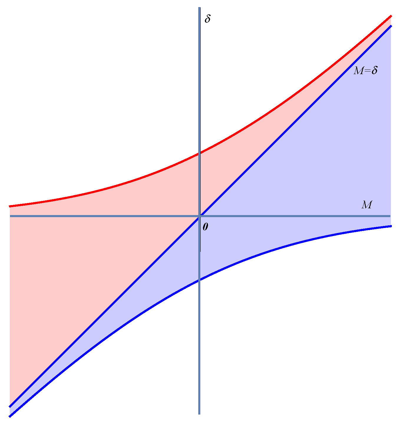
Moreover

$$G(1,1,1)=0 \mathrm{and} G(t,s,1)<0 \mathrm{for} \mathrm{all} (t,s)\in (I\times I)\backslash \left\{\right(1,1\left)\right\}$$

and

$$G(0,0,-1)=0 \mathrm{and} G(t,s,-1)>0 \mathrm{for} \mathrm{all} (t,s)\in (I\times I)\backslash \left\{\right(0,0\left)\right\}.$$

Figure 1 shows the regions where the function G maintains a constant sign.