Article

The Real-Life Application of Differential Evolution with a Distance-Based Mutation-Selection

Department of Informatics and Computers, Faculty of Science, University of Ostrava, 30. Dubna 22, 70103 Ostrava, Czech Republic
Mathematics 2021, 9(16), 1909; https://doi.org/10.3390/math9161909
Submission received: 1 July 2021 / Revised: 2 August 2021 / Accepted: 4 August 2021 / Published: 10 August 2021
(This article belongs to the Special Issue Evolutionary Algorithms in Engineering Design Optimization)

Abstract

:
This paper proposes the real-world application of the Differential Evolution (DE) algorithm using, distance-based mutation-selection, population size adaptation, and an archive for solutions (DEDMNA). This simple framework uses three widely-used mutation types with the application of binomial crossover. For each solution, the most proper position prior to evaluation is selected using the Euclidean distances of three newly generated positions. Moreover, an efficient linear population-size reduction mechanism is employed. Furthermore, an archive of older efficient solutions is used. The DEDMNA algorithm is applied to three real-life engineering problems and 13 constrained problems. Seven well-known state-of-the-art DE algorithms are used to compare the efficiency of DEDMNA. The performance of DEDMNA and other algorithms are comparatively assessed using statistical methods. The results obtained show that DEDMNA is a very comparable optimiser compared to the best performing DE variants. The simple idea of measuring the distance of the mutant solutions increases the performance of DE significantly.

1. Introduction

The solving of global optimisation problems is frequently needed in many areas of research, industry, and engineering where minimal or maximal cost values are required. In general, a global optimisation problem is specified in the search space Ω which is limited by its boundary constraints, Ω = j = 1 D [ a j , b j ] , a j < b j . The objective function f is defined in all x Ω and the point x * for f ( x * ) f ( x ) , x Ω is the solution of the global optimisation problem.
In this study, several engineering optimisation problems are used to illustrate the performance of both existing ( well-known) and newly proposed optimisation methods. The motivation and aim is to show the efficiency of the newly proposed optimisation algorithms. Achieving an optimal solution for engineering problems is a very popular research area [1]. Generally, the real-life application of optimisation methods is extremely important in many fields of industry, energy, and scheduling, etc. [2].
In addition to the area of engineering optimisation problems, the field of industrial economics is also very popular. In 2019, Dosi et al. introduced a comprehensive theoretical survey of the history of agent-based macroeconomics [3]. The authors critically discussed the issues found in macroeconomics from different points of view. The authors recommended the direct cooperation of agent-based macroeconomics with financial institutions. In 2020, Bellomo et al. introduced a theoretical cooperation between evolutionary theory and the theory of active particles [4]. The authors deeply analysed areas of evolutionary landscapes and the interactions found in endogenous systems which resulted in a model of differential equations. The results of the simulations showed the potential of their proposed approach in aiding the cooperation between states and private companies.
There are various optimisation approaches to find the minimal (maximal) function value of objective functions. The biggest group of optimisation methods is called the Evolutionary Algorithms (EAs), which are inspired by natural systems. One of the most frequently used EA is the Differential Evolution (DE) algorithm [5]. The high popularity of the DE algorithm is based on its simplicity and efficiency. Over more than 15 years, a lot of powerful DE variants have been developed and studied very intensively [6,7,8]. Despite the efficiency of DE, there is still not one specific variant of the optimisation algorithm which is possible to solve all global optimisation problems in the most efficient way (No Free Lunch theorem [9]).

Differential Evolution

Differential evolution was introduced by Storn and Price as a simple and efficient optimisation algorithm in 1996 [5]. DE is a population-based optimisation algorithm that uses three numerical control parameters. The main idea of DE is as follows. In the beginning, the population of N individuals (D-dimensional vectors) is generated randomly in Ω and evaluated by the objective function f. After initialisation, the development of the population is performed from generation to generation until the stopping condition is met. The development of the individuals in the population is controlled by evolutionary operators—mutation, crossover, and selection. A new trial individual (offspring) y i is derived from the current point x i as follows. A mutated individual u i is constructed from the current individual using mutation. There are several well-known mutation variants, the most widely-used mutation variant in DE is denoted rand/1 (1), where r 1 , r 2 , r 3 are randomly selected mutual indices from [ 1 , N ] , different from i.The parameter F ( 0 , 2 ] is called a scale factor.
u = x r 1 + F · ( x r 2 x r 3 )
After mutation, a crossover operation is performed. Here, elements of the original x i and the mutated individuals u i are used for a new offspring solution— y i . The most widely used crossover variant is known as binomial crossover (2), where the crossover ratio CR ( 0 , 1 ) controls the number of elements from a mutated individual selected for a trial solution.
y i , j = u i , j , i f r a n d j ( 0 , 1 ) CR o r j = r a n d j ( 1 , D ) x i , j , otherwise .
A new individual y i is evaluated by a cost function and it replaces the parent individual x i in the population if it is better, f ( y i ) f ( x i ) . This evolutionary operation is known as selection. When standard canonical DE is used for solving complex optimisation problems or large scale problems with high dimensions D, its efficiency is worse. The issue is mainly caused by the fixed values of the control parameters— N , CR , F . Then, the adaptive approach of the DE control parameters’ values helps to solve various optimisation tasks. A lot of successful adaptive DE variants have been introduced and applied to real-world problems [6,7,8].
In this paper, a new DE variant based on a distance-based selection of mutation individuals, using an archive of old-good solutions and a population-size reduction mechanism, was applied to real-world problems. The main motivation for using the new algorithm was derived from an attempt to control the speed of convergence in the DE by the proper selection of a mutation individual [10,11]. Euclidean distance is employed to select the correct mutation individual from a triplet based on the current stage of the algorithm. Additionally, using historical yet correct, solutions in a reproduction process can enhance the ability to avoid the local minimal area. Finally, changing the population size during the search (from a bigger value to a smaller value) enables the support of exploration in early generations and exploitation in later generations. The most important aspect of the research is the practical use of the proposed optimisation methods for real-world problems. Therefore, three real-world engineering problems and 13 constrained problems were used to evaluate the proposed DE and compare the results with other state-of-the-art DE variants.
The rest of the paper is organised as follows. The newly proposed DE variant is presented in Section 2. The real-world problems and experimental settings are represented in Section 3. The results obtained from the experimental study are presented and discussed in Section 4. The paper is briefly concluded in Section 5.

2. A Novel DE with Distance-Based Mutation-Selection (DEDMNA)

In this section, a DE variant with Distance-based Mutation-selection, population size (N) reduction, and the use of an archive of old-good solutions (DEDMNA) is introduced. The main motivation for this approach is to manage the speed of convergence in the DE algorithm because the selection of the proper mutation operation significantly influences the ability to increase or decrease the population diversity.
In 2012, Liang et al. proposed a new DE variant with a distance-based selection approach [12]. Here, newly generated solutions are based on the Euclidean distance of an individuals’ cost functions. A weakness of this approach is found in the necessity for the evaluation of the individuals. This is because it is typically the most time-consuming operation during the optimisation process.
In 2017, Gosh et al. proposed a DE variant with a distance-based mutation scheme using the central tendency of the population [13]. The Manhattan distance of the parent and offspring solution was applied to prioritise newly generated solutions with worse quality. The mechanism proposed a higher level of population diversity during the search.
In 2020, Liang et al. presented a novel DE algorithm based on the function value of the Euclidean-distance ratio [14]. This ratio reflects the function value and distance between two individuals in the population, and it is computed for the whole population. Therefore, the parent individuals are selected by roulette using the ratio values. The results of their experiments showed an increased efficiency in some classification problems.

2.1. Proper Mutation Variants for Convergence-Control

Standard DE uses mutation and crossover operations to generate new solutions to produce the next generation. There are many mutation variants, and preliminary results show that various mutation variants perform significantly differently [15]. Therefore, a couple of well-performing mutation variants which provide a variety of convergence-speeds were selected. Preliminary experimental results [10] and a theoretical analysis [11] provide an evaluation of DE mutation based on the speed of convergence. Based on preliminary experiments, the DE mutation variants rand/1 (1), best/2 were assessed as a balanced set of fast-converging and diversity-keeping mutation variants.
u = x b e s t + F · ( x r 1 x r 2 ) + F · ( x r 3 x r 4 )
u = x r 1 + F · ( x b e s t x r 1 ) + F · ( x r 2 x r 3 )
where x r 1 , x r 2 , x r 3 , x r 4 are mutually different points r 1 r 2 r 3 r 4 i and x best is best point of P.

2.2. Distance-Based Mutation-Selection Mechanism

The newly proposed DE with a distance-based approach is based on a previously designed DEMD variant [16]. The original DEMD uses only a distance-based mutation-selection approach and a control parameter adaptation approach. To improve the original DEMD, a linear population size reduction approach and an archive for old solutions were employed in our research. Here, more details of the original DEMD and its new enhanced variant are provided.
The main motivation for using the original DEMD was the control of the convergence ability (speed) of the DE algorithm. For each individual x i in population P, three mutation individuals are generated using the three mutation variants as discussed above. Then, the most proper mutation individual is selected for the crossover and selection, using the standard Euclidean distance, with respect to the current stage of the search process (exploration or exploitation). Note that where the CoDE variant [17] selects one of the three trial individuals evaluated by the cost function, the proposed DEDMNA uses the Euclidean distance between the coordinates of the points in the population. Therefore, the computational costs of the DEDMNA approach are substantially lower because the function evaluation of the individuals is a computationally expensive operation.
At the beginning of DEDMNA, a population of P of N individuals x i , i = 1 , 2 , , N is generated randomly in Ω and evaluated by objective function. Next, for each individual x i from P, a new solution y i is generated. The reproduction process of DEDMNA is divided into two phases—exploration and exploitation. The exploration phase is performed in the early generations of DEDMNA, and it keeps the coarse detection of potentially good regions of Ω . In this phase, for each x i three new mutant vectors u 1 , u 2 , and u 3 are produced using (1), (3) and (4) mutations. Subsequently, a mutation point with the least Euclidean distance between the mutation individuals and the current position x i is selected to choose the proper mutation individual and to achieve a better exploration of Ω . The second, exploitation, phase is controlled by (5), and the mutation point of the triplet of mutation individuals u 1 , u 2 , and u 3 with the least Euclidean distance between the mutation individuals and the best individual x best is selected to choose the proper mutation individuals and maintain a better exploitation ability.
dist = { j = 1 D ( u k , j x i , j ) 2 , if   FES / maxFES < rand j = 1 D ( u k , j x best , j ) 2 otherwise , k = 1 , 2 , 3 .
where FES is the current number of depleted function evaluations and maxFES the maximum FES for one run. Next, a new trial individual y i is developed using a standard binomial crossover (2).
It is clear that setting the control parameters F and CR are crucial for the efficiency of the DEDMNA algorithm. In DEDMNA, an adaptive approach to changing the values of F and CR during the search process is employed. Simply, the values of CR are generated randomly, uniformly from the interval ( 0 , 1 ) , and independently for each point in P. Furthermore, the value of CR i is randomly re-sampled if it has a small probability of 0.1 . The adaptive mechanism for the values of F depend on the current phase. In the early exploration phase, the values of F i are computed as a random permutation of length N divided by N for each point from P. Such values equidistantly cover the interval ( 0 , 1 ) . In the late exploitation phase, values of F i are sampled as a random number from the uniform interval ( 0 , 1 ) . In both phases, the F i values are randomly assigned to individuals of P and modified by F i = F i + 0.1 r a n d . Such a modification guarantees slightly varying values in each generation. Similar adaptation mechanisms for the DE control parameters were also used in the original algorithms [18,19].

2.3. Archive of Historically Good Solutions

To simplify the use of archived historical solutions in A, point x r 3 (see (1), (3) and (4)) is randomly selected from P A (the remaining points for mutation are selected solely from P). It means that when the archive is fully written, the randomly selected individual x r 3 has a 50 % chance from being from P and a 50 % chance from A.

2.4. Population Size Adaptation

Preliminary experiments showed that varying the population size during the search significantly increases the performance of the DE algorithm [20,21,22]. The population size N of the DEDMNA algorithm is linearly reduced during the search process from a bigger value at the beginning to a smaller value at the end. After each generation, the current proper population size (based on linear dependency) is computed (6). When the current population size N differs from the needed value, the population size is reduced:
N = round [ ( N min N init maxFES ) FES + N init ] ,
where FES is the current number of function evaluations, N init is the initial population size, N min represents the size of population at the end of the search process (counted by the total number of maxFES function evaluations).

3. Experimental Settings

The proposed DEDMNA algorithm was applied to three engineering problems and 13 constrained problems. The results from DEDMNA were compared with six state-of-the-art DE variants.

3.1. State-of-the-Art Variants in Comparison

Six state-of-the-art DE variants were selected for an experimental comparison to assess the performance of the proposed DEDMNA variant. A brief description of the methods in a chronological manner follows.
In 2006, Brest et al. proposed a simple and efficient adaptive DE variant (jDE) [18]. jDE uses a DE/rand/1/bin strategy with an adaptive approach of F and CR. Each individual has separate values of F and CR, and in each generation, it is regenerated with a probability of 0.1 . More details of the efficient jDE method can be found in [18].
In 2009, Qin et al. proposed a DE algorithm with strategy adaptation (SaDE) [23]. In Sade, four mutation strategies (rand/1/bin, rand/2/bin, rand-to-best/2/bin, and current-to-rand/1) are used for generating new trial solutions. The strategy to be applied is selected by roulette based on the success and failure of previous LP generations. Each strategy has the same probability set to 1 / 4 , i.e., all the strategies have an equal probability of being selected.
In 2013, Tanabe and Fukunaga introduced the Success-History Based Parameter Adaptation for Differential Evolution (SHADE) [24] which was the best performing DE variant in the CEC 2013 competition. SHADE is derived from JADE [25], where the main difference between SHADE and the original JADE is a different history-based adaptation of the control parameters F and CR. Both algorithms use a current-to-pbest mutation strategy where one parent individual is selected from P A . The SHADE algorithm is abbreviated in the results of this paper as SHA.
In 2014, Wang et al. proposed a new DE variant using covariance-matrix learning and bimodal parameter settings (CoBiDE and CoBi in results) [26]. CoBiDE advances the canonical DE in two new aspects–the covariance-matrix crossover (based on Eigenvectors of the population) and bimodal sampling of the control parameters, which distinguishes between exploration and exploitation. The authors of CoBiDE supposed a higher performance in problems defined by rotated objective functions. The Eigenvector crossover is controlled by two control parameters pb = 0.4 is the probability of using the Eigenvector crossover (instead of the classic binomial crossover) in the whole population, and ps = 0.5 is the portion of the population used to determine the Eigenvectors. More details are provided in the original paper.
In 2015, Tang et al. introduced a DE with an Individual-Dependent Mechanism [19]. The search process in IDE is divided into explorative and exploitative phases. The dynamic setting of the F and CR values using the quality of the individuals is employed. Better individuals with lesser objective function values have smaller values of F and CR and vice versa. In 2017, an advanced IDE variant was proposed with a novel mutation variant and diversity-based population size control (IDEbd) [27]. The details of the IDEbd method can be found in the original paper, and it is labelled simply by ‘IDE‘ in the results section of this paper.
In 2017, Brest et al. introduced an adaptive DE variant derived from the successful JADE, SHADE, and L-SHADE called jSO [21]. The jSO algorithm achieved second position in the CEC 2017 competition. jSO uses historical circle memories of length 5 containing the mean values for generating F and CR. In the first half of the jSO search process, higher values of CR are used. In the first 60% of evaluations, the values of F are kept under 0.7. jSO uses an advanced weighted current-to-pbest mutation. Finally, jSO uses a linear adaptation of the population size where the initial population size is N = 25 × D × log D . More details are available in [21].
In 2019, Brest et al. proposed a very efficient adaptive DE variant called jDE100 [28], In 2019, jDE100 was the optimisation algorithm with the best results in the CEC competition. The jDE100 algorithm is derived from jDE. In jDE100, two independent populations are used—one big and one small. Also, the initial values of the mutation and crossover are set to F = 0.5 and CR = 0.9 for each individual in both populations. After one generation of the big population, if the best solution for the jDE100 is in the big population, it is copied to the small population. Then, when the condition for the re-initialisation of the big population is satisfied, it is reset. Then several generations of the small population are performed (equally to the number of function evaluations of the big population), and also the reset condition is verified, and the best solutions are stored. More details regarding jDE100 can be found in the original paper.

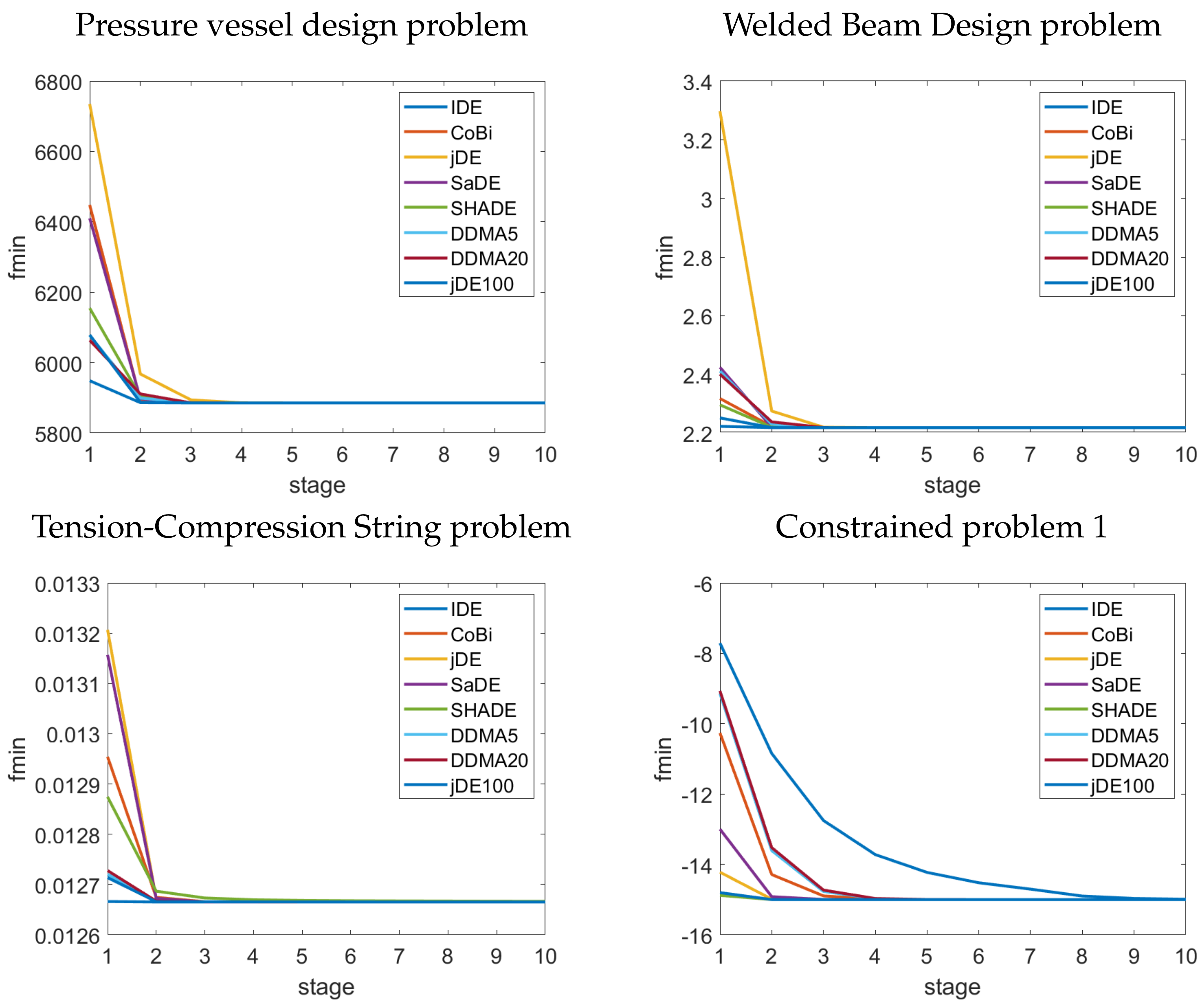
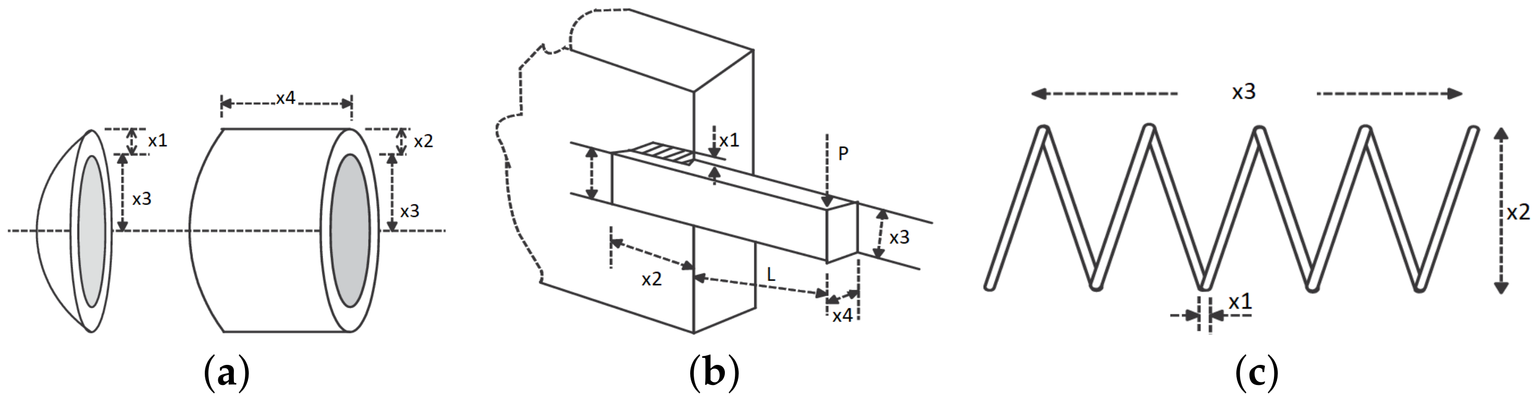
3.2. Well-Known Engineering Problems

The experimental comparison found here is based on three well-known engineering problems [29]. All the problems are related to minimisation, i.e., the global minimum point is the solution. The computational complexity of the problems are varied, and the dimensionality of the search space is ( D { 3 , 4 }). For each algorithm and problem, 25 independent runs were performed. Each algorithm stops when it achieves a predefined number of function evaluation, i.e., MaxFES = 150,000. A better insight into the results of the algorithms is provided by results achieved at MaxFES = 50,000 and MaxFES = 100,000. Finally, the individual of the final population with the least function value is the solution of the algorithm for the given problem.
In the pressure vessel design problem (labelled preved in results), the production costs represented by four parameters and constraints are minimised. The decision space area is represented by a four-dimensional real-valued space: x 1 defines the thickness of the head, x 2 is the thickness of the cylinder, x 3 is the inner radius, and x 4 is the length of the cylinder part (see Figure 1a)). The objective function is defined:
f ( y ) = 0.6224 x 1 x 3 x 4 + 1.7781 x 2 x 3 2 + 3.1661 x 1 2 x 4 + 19.84 x 1 2 x 3
with constraints:
y 1 = x 1 + 0.0193 x 3 0 y 2 = x 2 + 0.00954 x 3 0 y 3 = π x 3 2 x 4 4 3 π x 3 3 + 1 , 296,000 0 y 4 = x 4 240 0
The purpose of the second Welded Beam Design problem (labelled welded in results) is to achieve the best production cost regarding a set of project constraints. An illustration of this problem is depicted in Figure 1b). The problem variables are—the weld thickness ( x 1 ) length ( x 2 ), height ( x 3 ), and thickness of the bar ( x 4 ).
f ( y ) = 1.10471 x 1 2 x 2 + 0.04811 x 3 x 4 ( 14.0 + x 2 )
with settings:
t max = 13,600 s max = 30,000 d max = 0.25 M = P ( L + x 2 2 ) R = 0.25 ( x 2 2 + ( x 1 + x 3 ) 2 ) P = 6000 L = 14 E = 3 × 10 6 G = 12 × 10 6 J = 2 2 x 1 x 2 ( x 2 2 / 12 + 0.25 ( x 1 + x 3 ) 2 ) P c = ( 4.013 E ( 6 L 2 ) ) x 3 x 4 3 ( 1 0.25 x 3 E / G / L ) t 1 = P / ( 2 x 1 x 2 ) , t 2 = M R / J t = 1 2 + t 1 t 2 x 2 / R + t 2 2 s = 6 P L / ( x 4 x 3 2 ) , d = 4 P L 3 / ( E x 4 x 3 3 )
and constraints:
y 1 = t t max y 2 = s s max y 3 = x 1 x 4 y 4 = 0.10471 x 1 2 + 0.04811 x 3 x 4 ( 14.0 + x ) ) 5.0
In the Tension-Compression String problem (labelled tecost in results), the weight of the spring is minimised. The problem variables of the tecost problem are the wire diameter ( x 1 ), the mean coil diameter ( x 2 ), and the number of active coils ( x 3 ). The tecost problem is restricted by the constraints of shear stress, surge frequency, and minimum deflection (Figure 1c)). The objective function is:
f ( y ) = x 1 2 x 2 ( x 3 + 2 )
with constraints:
y 1 = 1 x 2 3 x 3 71,785 x 1 4 y 2 = 4 x 2 2 x 1 x 2 12,566 x 1 3 ( x 2 x 1 ) ) + 1 5108 x 1 2 1 y 3 = 1 140.45 x 1 / ( x 3 x 2 2 ) y 4 = x 1 + x 2 1.5 1

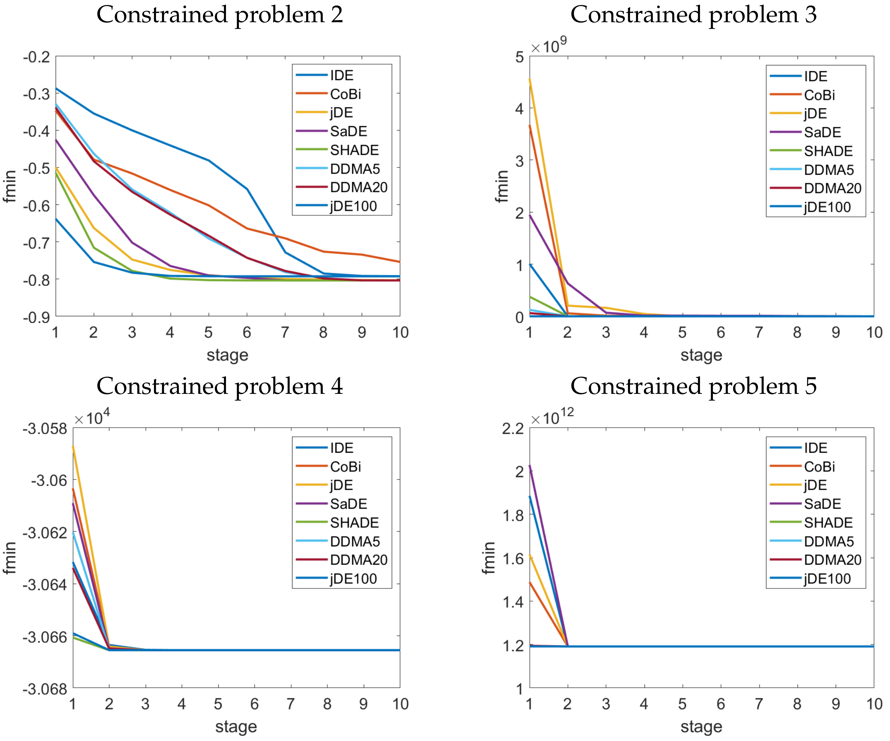
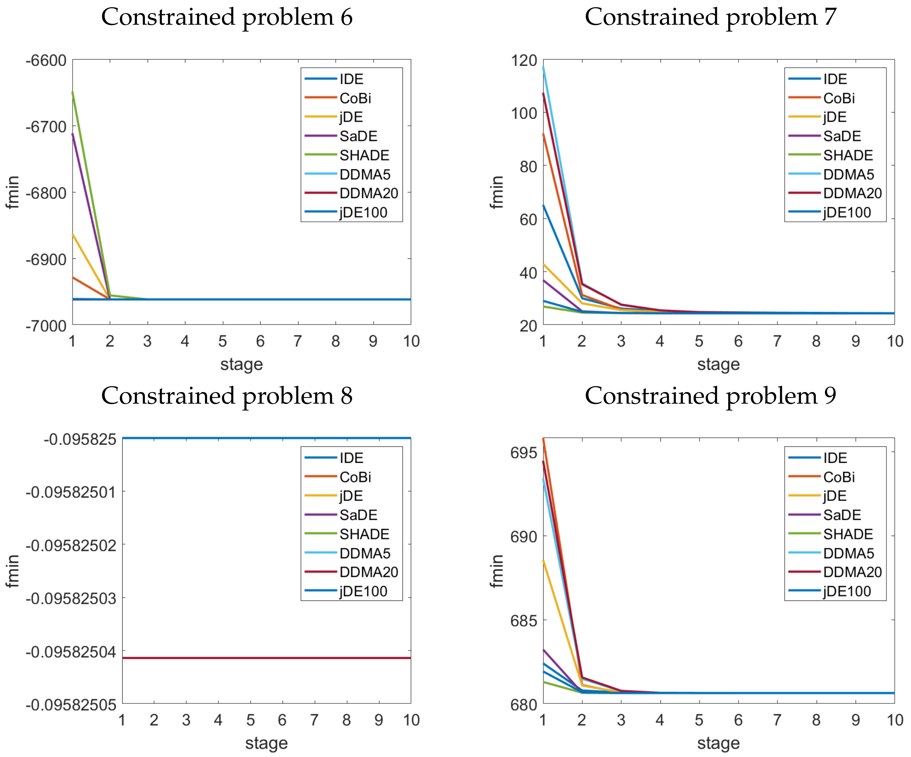
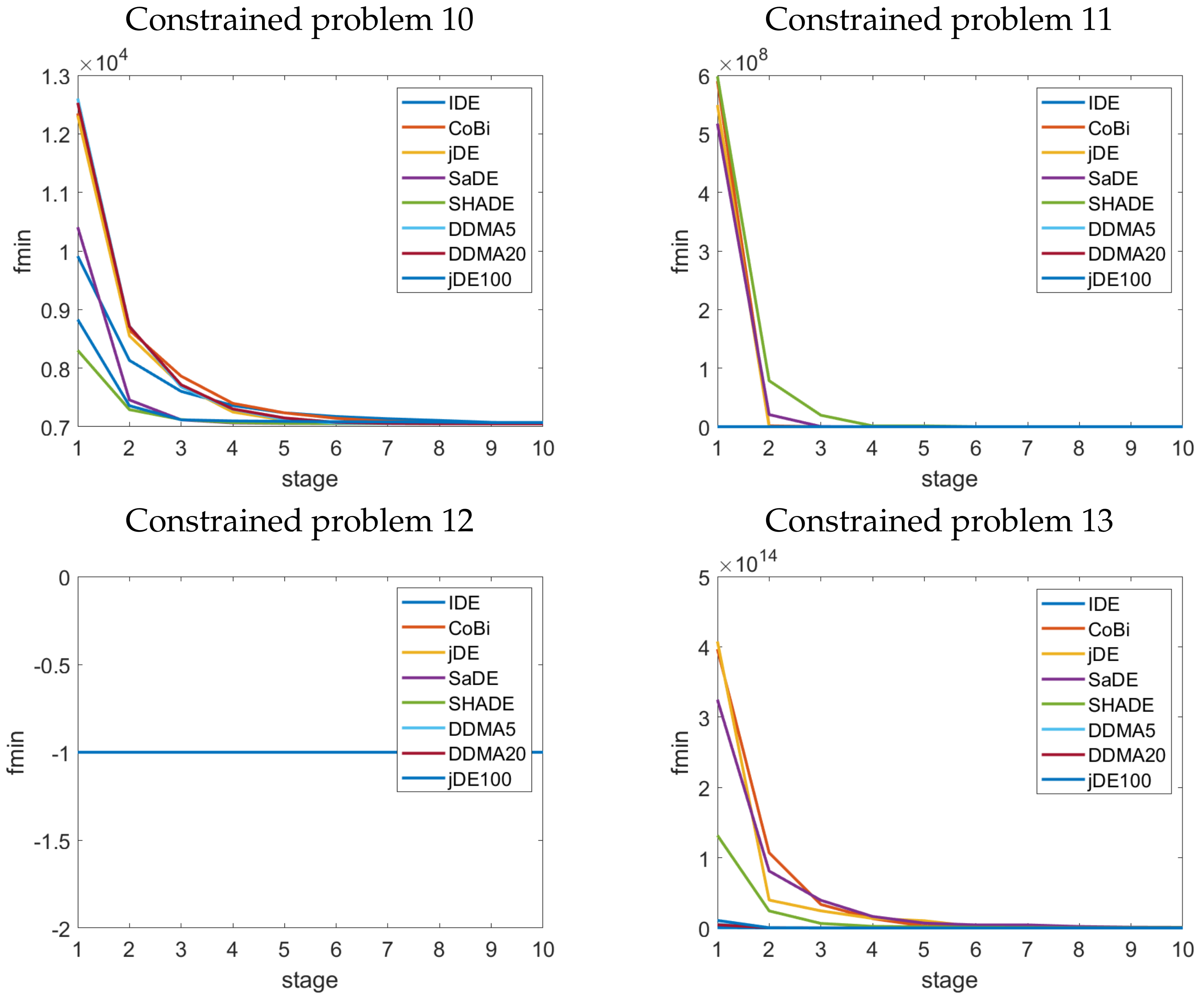
3.3. Constrained Optimisation Problems

Real-world problems are very often defined as constrained optimisation problems. The constrained conditions (based on equality or inequality) specify more accurate areas for the allowed values of optimised variables. Therefore, a set of 13 minimisation constrained problems are used in experiments to distinguish more and less efficient methods. Details and definitions of the objective functions of the constrained problems are available in [29]. The constrained problems are labelled p 1 p 13 following the order of the original report. The dimensionality of the search space is D ( 2 , 20 ).
All algorithms and problems are implemented and experimentally compared in a Matlab 2020b environment. All computations were carried out on a standard PC with Windows 10, Intel(R) Core(TM)i7-9700 CPU 3.0 GHz, 16 GB RAM. For each algorithm and problem maxFES = 100,000 and is the stopping condition of the search, and 25 independent runs were performed to achieve statistically significant results. The population size of all algorithms is N = 90 . The control parameters are minimal population size ( N min = 5 , 20 ), initial population size ( N init = r o u n d ( 25 l o g ( D ) D [21]), and the size of the archive is equal to the population size N. Based on the final population size values, two different DEDMNA variants are labelled in the results as DDMA 5 and DDMA 20 . The control parameters for the state-of-the-art algorithms used in this comparison, follow the recommended settings from the original papers.

4. Results

In this paper, two variants of the novel DEDMNA algorithm are compared with six state-of-the-art DE variants when solving three engineering and 13 constrained problems. At first, the performance of all nine algorithms is compared using the Friedman test. This method provides the mean ranks of the algorithms in comparison using the median values of the best-achieved function values. The best-achieved solution for each algorithm was recorded in ten phases of the search. The mean ranks for each algorithm and problem for the ten phases are in Table 1. The mean ranks represent the overall performance of the algorithm, including all 16 problems. The algorithms are ordered based on the mean rank in the final 10th phase ( MR s t = 10 ). The mean rank of the best algorithm is printed bold and underlined, the second-best is printed bold, and the algorithm in the third position is underlined. In the last column, the achieved significance level of the Friedman tests is presented. If the null hypothesis is rejected, symbol of ( p < 0.001 ), ( p < 0.01 ), and ∗ ( p < 0.05 ) is presented. Otherwise, symbol of ≈ demonstrate cases, where the null hypothesis is not rejected.
The null hypothesis is rejected only in the first two phases; the performance of the algorithms in the remaining phases is rather similar. Very interesting information is provided by the development of the mean rank values for each algorithm during the progression of stages. In the early phases, jDE100 and SHADE variants are well-performing. The best results, including all 16 problems in the last two (final) phases, were achieved by the newly proposed DEDMNA 20 and DEDMNA 5 . It highlights the effective performance of the proposed DEDMNA method. A better insight into the mean rank comparison is provided by the plots of the mean ranks in Figure 2. The performance of jDE100 decreases during the search, whereas the efficiency of the DEDMNA algorithm increases (especially for DEDMNA 20 ).
A more detailed comparison is provided by the Wilcoxon rank-sum tests. The test is applied to compare the results of two algorithms with one problem. The reference method is DEDMNA 20 (best mean rank from the Friedman test), and it is compared with the seven remaining counterparts. In Table 2 and Table 3, the median values of all algorithms and problems are shown, including the significance from the Wilcoxon rank-sum tests (‘−’ denotes the better performance of a counterpart method, ‘+’ shows the better performance of DEDMNA 20 , and ‘≈’ is for similar results). Mostly, the median values of all the compared algorithms are very similar to the achieved true solution.
For a better comparison of the algorithms, the counts of better, similar, and worse results for the reference DEDMNA 20 algorithm are depicted in the last row of the tables.
Compared to IDEbd (labelled IDE), DEDMNA 20 performs better in five constrained problems and is worse in one constrained and one engineering problem. CoBiDE is outperformed by the reference method in seven problems, and it performs better in three problems. DEDMNA 20 outperforms jDE in four constrained problems and never performs worse. DEDMNA 20 is better in six constrained problems and worse in three constrained problems and three engineering problems, compared to SaDE. SHADE is able to outperform the reference method in three constrained problems, and it performs worse in three constrained and one engineering problem. The results of the two DEDMNA variants are very similar, and each is better in one problem. DEDMNA 20 outperforms jDE100 in eight constrained problems, and it is worse in two engineering problems and two constrained problems.
More insight into the algorithms’ performance is provided by convergence plots for all 16 problems (see Figure 3, Figure 4, Figure 5 and Figure 6). It is clear that in constrained problems 8 and 12, all the algorithms converge in the first phase. In the remaining problems, the convergence process takes some time. An interesting observation is the convergence of constrained problem 2, where the curves of the best algorithms’ solutions differ to the last phase. The worst convergence is with CoBiDE, whereas very good results are provided by DEDMNA 20 .

5. Conclusions

In this experimental comparison, two newly proposed DEDMNA variants are compared with six state-of-the-art DE variants when solving three engineering problems and 13 constrained problems. The results of the Friedman tests show that the DEDMNA variant provides the best performance in the last phase of the search, whereas the successful jDE100 variant performs better in the early phases of the search. The better results for DEDMNA, with a bigger final population size, indicates the necessity for higher diversity during the search process.
The counts of better and worse results from the Wilcoxon rank-sum test show that the new DEDMNA variant is able to be comparable with optimised state-of-the-art methods when applied to real-world problems. Despite this, all algorithms achieved mostly quite similar results, which illustrate the ability of the methods to determine the area of the true solution. The Proposed DEDMNA variant was successfully applied to the current CEC 2021 competition, and it achieves a very promising performance compared to the state-of-the-art DE algorithms from the preliminary experiments. This finding is very promising for the future development of new optimisation methods. The performance of DEDMNA will be studied and further tuned in future research.

Funding

This research was funded by Internal Grant Agency of University of Ostrava grant number SGS17/PrF-MF/2021.

Institutional Review Board Statement

Not applicable.

Informed Consent Statement

Not applicable.

Data Availability Statement

All data was measured in Matlab during the experiments.

Conflicts of Interest

The funders had no role in the design of the study; in the collection, analyses, or interpretation of data; in the writing of the manuscript, or in the decision to publish the results.

References

  1. Rhinehart, R.R. Engineering Optimization: Applications, Methods and Analysis; John Wiley & Sons: Hoboken, NJ, USA, 2018. [Google Scholar]
  2. Fujisawa, K.; Shinano, Y.; Waki, H. Optimization in the Real World: Toward Solving Real-World Optimization Problems; Mathematics for Industry, Springer: Berlin/Heidelberg, Germany, 2016. [Google Scholar]
  3. Dosi, G.; Roventini, A. More is Different ... and Complex! The Case for Agent-Based Macroeconomics. J. Evol. Econ. 2019, 29, 1–37. [Google Scholar] [CrossRef] [Green Version]
  4. Bellomo, N.; Dosi, G.; Knopoff, D.A.; Virgillito, M.E. From particles to firms: On the kinetic theory of climbing up evolutionary landscapes. Math. Model. Methods Appl. Sci. 2020, 30, 1441–1460. [Google Scholar] [CrossRef]
  5. Storn, R.; Price, K.V. Differential evolution—A Simple and Efficient Heuristic for Global Optimization over Continuous Spaces. J. Glob. Optim. 1997, 11, 341–359. [Google Scholar] [CrossRef]
  6. Das, S.; Mullick, S.; Suganthan, P. Recent advances in differential evolution—An updated survey. Swarm Evol. Comput. 2016, 27, 1–30. [Google Scholar] [CrossRef]
  7. Das, S.; Suganthan, P.N. Differential Evolution: A Survey of the State-of-the-Art. IEEE Trans. Evol. Comput. 2011, 15, 27–54. [Google Scholar] [CrossRef]
  8. Neri, F.; Tirronen, V. Recent advances in differential evolution: A survey and experimental analysis. Artif. Intell. Rev. 2010, 33, 61–106. [Google Scholar] [CrossRef]
  9. Wolpert, D.H.; Macready, W.G. No Free Lunch Theorems for Optimization. IEEE Trans. Evol. Comput. 1997, 1, 67–82. [Google Scholar] [CrossRef] [Green Version]
  10. Jeyakumar, G.; Shanmugavelayutham, C. Convergence analysis of differential evolution variants on unconstrained global optimization functions. Int. J. Artif. Intell. Appl. (IJAIA) 2011, 2, 116–127. [Google Scholar] [CrossRef]
  11. Zaharie, D. Differential Evolution: From Theoretical Analysis to Practical Insights. In MENDEL 2012, 18th International Conference on Soft Computing, 27–29 June 2012; University of Technology: Brno, Czech Republic, 2013; pp. 126–131. [Google Scholar]
  12. Liang, J.; Qu, B.; Mao, X.; Chen, T. Differential Evolution Based on Fitness Euclidean-Distance Ratio for Multimodal Optimization. In Emerging Intelligent Computing Technology and Applications; Huang, D.S., Gupta, P., Zhang, X., Premaratne, P., Eds.; Springer Berlin Heidelberg: Berlin/Heidelberg, Germany, 2012; pp. 495–500. [Google Scholar]
  13. Ghosh, A.; Das, S.; Mallipeddi, R.; Das, A.K.; Dash, S.S. A Modified Differential Evolution With Distance-based Selection for Continuous Optimization in Presence of Noise. IEEE Access 2017, 5, 26944–26964. [Google Scholar] [CrossRef]
  14. Liang, J.; Wei, Y.; Qu, B.; Yue, C.; Song, H. Ensemble learning based on fitness Euclidean-distance ratio differential evolution for classification. Nat. Comput. 2021, 20, 77–87. [Google Scholar] [CrossRef]
  15. Bujok, P.; Tvrdík, J. A Comparison of Various Strategies in Differential Evolution. In Proceedings of the MENDEL, 17th International Conference on Soft Computing, Brno, Czech Republic, 14–17 June 2011; pp. 48–55. [Google Scholar]
  16. Bujok, P. Improving the Convergence of Differential Evolution. In Numerical Analysis and Applications; Lecture Notes in Computer Science; Springer: Berlin/Heidelberg, Germany, 2016; pp. 248–255. [Google Scholar]
  17. Wang, Y.; Cai, Z.; Zhang, Q. Differential Evolution with Composite Trial Vector Generation Strategies and Control Parameters. IEEE Trans. Evol. Comput. 2011, 15, 55–66. [Google Scholar] [CrossRef]
  18. Brest, J.; Greiner, S.; Boškovič, B.; Mernik, M.; Žumer, V. Self-adapting Control Parameters in Differential Evolution: A Comparative Study on Numerical Benchmark Problems. IEEE Trans. Evol. Comput. 2006, 10, 646–657. [Google Scholar] [CrossRef]
  19. Tang, L.; Dong, Y.; Liu, J. Differential Evolution With an Individual-Dependent Mechanism. IEEE Trans. Evol. Comput. 2015, 19, 560–574. [Google Scholar] [CrossRef] [Green Version]
  20. Tanabe, R.; Fukunaga, A.S. Improving the search performance of SHADE using linear population size reduction. In Proceedings of the IEEE Congress on Evolutionary Computation (CEC), Beijing, China, 6–11 July 2014; pp. 1658–1665. [Google Scholar]
  21. Brest, J.; Maučec, M.S.; Bošković, B. Single Objective Real-Parameter Optimization: Algorithm jSO. In Proceedings of the 2017 IEEE Congress on Evolutionary Computation (CEC), Donostia, Spain, 5–8 June 2017; pp. 1311–1318. [Google Scholar]
  22. Polakova, R.; Tvrdik, J.; Bujok, P. Differential evolution with adaptive mechanism of population size according to current population diversity. Swarm Evol. Comput. 2019, 50, 100519. [Google Scholar] [CrossRef]
  23. Qin, A.K.; Huang, V.L.; Suganthan, P.N. Differential Evolution Algorithm With Strategy Adaptation for Global Numerical Optimization. IEEE Trans. Evol. Comput. 2009, 13, 398–417. [Google Scholar] [CrossRef]
  24. Tanabe, R.; Fukunaga, A.S. Success-history based parameter adaptation for Differential Evolution. In Proceedings of the IEEE Congress on Evolutionary Computation (CEC), Cancun, Mexico, 20–23 June 2013; pp. 71–78. [Google Scholar]
  25. Zhang, J.; Sanderson, A.C. JADE: Adaptive Differential Evolution With Optional External Archive. IEEE Trans. Evol. Comput. 2009, 13, 945–958. [Google Scholar] [CrossRef]
  26. Wang, Y.; Li, H.X.; Huang, T.; Li, L. Differential evolution based on covariance matrix learning and bimodal distribution parameter setting. Appl. Soft Comput. 2014, 18, 232–247. [Google Scholar] [CrossRef]
  27. Bujok, P.; Tvrdík, J. Enhanced individual-dependent differential evolution with population size adaptation. In Proceedings of the 2017 IEEE Congress on Evolutionary Computation (CEC), Donostia, Spain, 5–8 June 2017; pp. 1358–1365. [Google Scholar]
  28. Brest, J.; Maučec, M.S.; Bošković, B. The 100-Digit Challenge: Algorithm jDE100. In Proceedings of the 2019 IEEE Congress on Evolutionary Computation (CEC), Wellington, New Zealand, 10–13 June 2019; pp. 19–26. [Google Scholar] [CrossRef]
  29. Hedar, A.R. Global Optimization Test Problems. Available online: http://www-optima.amp.i.kyoto-u.ac.jp/member/student/hedar/Hedar_files/TestGO_files/Page422.htm (accessed on 30 June 2021).
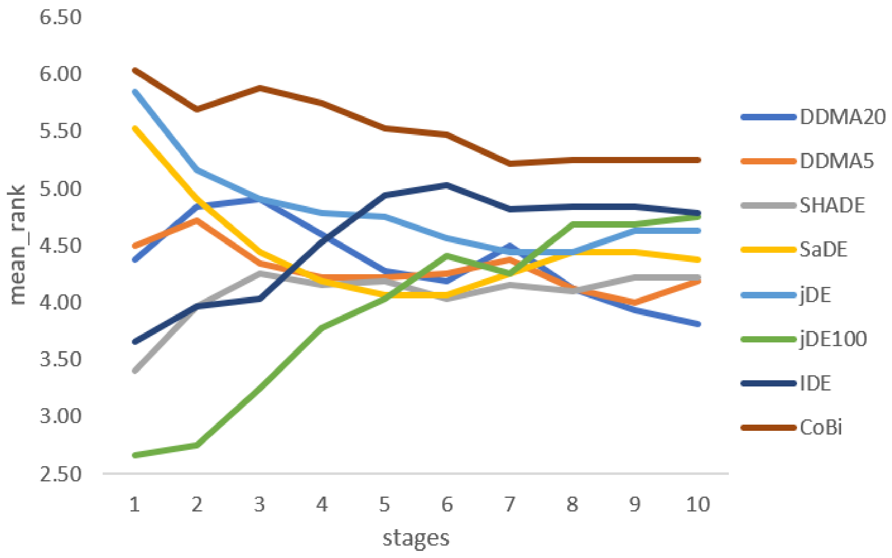
Figure 1. (a) Pressure vessel design problem, (b) Welded beam design problem, and (c) Tension-compression string problem.
Mathematics 09 01909 g001
Figure 2. Illustration of the algorithms’ mean ranks from the Friedman tests.
Mathematics 09 01909 g002
Figure 3. Convergence plots of the algorithms in comparison.
Mathematics 09 01909 g003
Figure 4. Convergence plots of the algorithms in comparison.
Mathematics 09 01909 g004
Figure 5. Convergence plots of the algorithms in comparison.
Mathematics 09 01909 g005
Figure 6. Convergence plots of the algorithms in comparison.
Mathematics 09 01909 g006
Table 1. Mean ranks of all algorithms from the Friedman tests computed for each stage independently.
MR st DDMA 20 DDMA 5 SHASaDEjDEjDE100IDECoBiSig.
14.384.503.415.535.842.663.666.03***
24.844.723.974.915.162.753.975.69*
34.914.344.254.444.913.254.035.88
44.594.224.164.194.783.784.535.75
54.284.224.194.064.754.034.945.53
64.194.254.034.064.564.415.035.47
74.504.384.164.254.444.254.815.22
84.134.134.094.444.444.694.845.25
93.944.004.224.444.634.694.845.25
103.814.194.224.384.634.754.785.25
Table 2. Median values for each algorithm and problem, with significance from the Wilcoxon rank-sum tests.
FunDDMA 20 IDECoBijDESaDE
preved5885.3335885.33285885.3335885.3335885.33
(≈)(≈)(≈)( )
welded2.2181512.2181512.2181512.2181512.21815
(≈)(≈)(≈)( )
tecost0.0126650.0126650.0126650.0126650.012665
( )( )(≈)( )
p1−15−14.99−15−15−15
(+++)(≈)(≈)(≈)
p2−0.8049−0.792−0.754−0.803−0.804
(+++)(+++)(+)(≈)
p3−0.02377−0.25338−1.04 × 10 4 −3.00 × 10 6 −5.00 × 10 6
( )(+++)(+++)(+++)
p4−30665.5−30665.5−30665.5−30665.5−30665.5
(≈)(+++)(≈)(+++)
p51.19 × 10 12 1.19 × 10 12 1.19 × 10 12 1.19 × 10 12 1.19 × 10 12
(≈)( )(≈)( )
p6−6961.81−6961.81−6961.81−6961.81−6961.81
(≈)(+++)(≈)(+++)
p724.3069724.3521824.30724.3079824.3064
(+++)(≈)(++)( )
p8−0.09583−0.09583−0.095825−0.09583−0.095825
(≈)(+++)(≈)(+++)
p9680.6301680.63007680.63680.6301680.63
(+++)( )(≈)( )
p107049.427059.317054.687049.437049.41
(+++)(+++)(≈)(≈)
p110.74990.74990.74990.74990.9656
(≈)(≈)(≈)(+++)
p12−1−1−1−1−1
(≈)(≈)(≈)(≈)
p134.1 × 10 8 0.954563.25 × 10 9 1.44 × 10 10 8.95 × 10 11
( )(+)(++)(+++)
Σ 5/8/37/6/34/12/06/4/6
Table 3. Median values for each algorithm and problem, with significance from the Wilcoxon rank-sum tests.
FunDDMA 20 SHADEDDMA 5 jDE100
preved5885.3335885.3328(≈)5885.3328(≈)5885.330( )
welded2.2181512.2181509(≈)2.2181509(≈)2.21815( )
tecost0.0126650.012666(+++)0.012665(+)0.012665(≈)
p1−15−15(≈)−15(≈)−15(≈)
p2−0.80359−0.8036( )−0.8036(≈)−0.79256(+++)
p3−0.02377−0.0004899(+++)−0.02249(≈)−0.00268(+++)
p4−30665.5−30665.5387(≈)−30665.5387(≈)−30665.5(+++)
p51.19 × 10 12 1.19 × 10 12 (≈)1.19 × 10 12 (≈)1.19 × 10 12 ( )
p6−6961.81−6961.81388(≈)−6961.81388(≈)−6961.81(+++)
p724.3069724.30625( )24.30699(≈)24.3269(+++)
p8−0.09583−0.095823(≈)−0.09583(≈)−0.095825(+++)
p9680.6301680.630057(≈)680.630057(≈)680.633(+++)
p107049.427049.29( )7049.55(≈)7071.57(+++)
p110.74990.9401(+++)0.7499(≈)0.7499(≈)
p12−1−1(≈)−1(≈)−1(≈)
p134.1 × 10 8 5.07 × 10 11 (+++)0.97026(−)0.902( )
Σ 4/9/31/14/18/4/4
Publisher’s Note: MDPI stays neutral with regard to jurisdictional claims in published maps and institutional affiliations.

