Evolutionary Design of a System for Online Surface Roughness Measurements

Abstract

Surface roughness is one of the key characteristics of machined components as it affects the surface quality and, consequently, the lifetime of the components themselves. The most common method of measuring the surface roughness is contact profilometry. Although this method is still widely applied, it has several drawbacks, such as limited measurement speed, sensitivity to vibrations, and requirement for precise positioning of the measured samples. In this paper, machine vision, machine learning and evolutionary optimization algorithms are used to induce a model for predicting the surface roughness of automotive components. Based on the attributes extracted by a machine vision algorithm, a machine learning algorithm generates the roughness predictive model. In addition, an evolutionary algorithm is used to tune the machine vision and machine learning algorithm parameters in order to find the most accurate predictive model. The developed methodology is comparable to the existing contact measurement method with respect to accuracy, but advantageous in that it is capable of predicting the surface roughness online and in real time.

1. Introduction

Demands for increased productivity and product quality in highly competitive industries, such as the automotive industry, have necessitated the use of online systems for inspecting the quality of massively produced parts. One of the quality measures that is especially challenging for online examination is surface roughness of machined parts. Surface roughness is defined as an amplitude value measuring the vertical heights of the surface deviations from a reference line [1]. Inadequate surface roughness of machined parts can significantly affect the functionality of a product and can lead to a premature failure. Moreover, measurement of surface roughness in production can reduce machining costs, since the machining parameters, such as machining speed and the period between the changes of machining tools, can be appropriately chosen.

The most widely used method of surface roughness measuring is contact profilometry. This method uses a stylus type device that correlates displacements induced by surface irregularities to the surface roughness of the inspected specimen. The method is standardized and has been widely used in industrial laboratories and manufacturing industry [2]. The technology of contact profilometry is well developed and can provide measurements of surface roughness within the accuracy of a micrometer. However, this method has several drawbacks. Since the stylus tip must be brought into contact with the measured specimen, the measured surface can be altered by scratches. Moreover, this method is time-consuming and sensitive to vibrations, and therefore not suitable for online measurements in high-volume production processes. More details about stylus-based roughness measurements and their advantages and shortcomings can be found in [3].

To overcome the drawbacks of contact methods, several non-contact methods, such as optical profilometry, scanning electron microscopy, atomic force microscopy, and laser scanning microscopy, have been developed. These methods can provide very accurate measurements of surface roughness and are becoming increasingly popular, also in the automotive industry [4]. However, the methods still require the preparation of adequate samples, are sensitive to vibrations and the measuring apparatuses are expensive. Consequently, none of these methods can be used for online and real-time surface roughness measurements.

This paper presents the development of a machine vision system for roughness evaluation of graphite commutator mounting holes. The graphite commutators are components of electric motors used in automotive fuel pumps. The final phase in the graphite commutator production is the precise turning of the commutator mounting hole to achieve an adequate hole inner diameter and surface roughness. Both characteristics, the diameter and roughness, are important for reliable operation of a fuel pump. Several online methods for measuring the inner diameter of holes are applicable; however, online roughness measurement of the hole surface roughness represents a major challenge.

Specifically, the work proposes combining machine vision (MV), machine learning (ML) and optimization methods to build a predictive model capable of determining the mounting hole roughness. The MV algorithm extracts the attributes from the commutator mounting hole surface that are used by ML to build a roughness predictive model. However, MV and ML methods depend on numerous parameters that notably affect the outcome and are hard to set to their optimum values. To overcome this limitation, an optimization algorithm is used to set the MV and ML algorithm parameters.

The paper is further organized as follows. Section 2 presents the related work in MV-based systems for measurement of surface roughness. The design and development of the online surface roughness measurement system are presented in Section 3. Section 4 describes the optimization methodology for automated tuning of MV and ML algorithm parameters in the development process. Section 5 describes the experimental setup and validation procedure used in the development. The experimental results are discussed in Section 6. Finally, Section 7 concludes the paper with a summary of findings and ideas for future work.

2. Related Work

The initial experiment with a setup similar to the one presented in this paper, combining MV, ML and optimization methods was carried out in [5]. The differential evolution (DE) [6] algorithm was used to search for optimal MV parameter settings, such as binary threshold and filter parameter values. Based on the attributes extracted from 300 images of the commutator mounting holes, the ML algorithm was employed to build classification and regression predictive models. The study found that in comparison to the domain expert this methodology always finds better MV parameter settings. In the classification task, the methodology was able to find a classification model of 100% accuracy in very few examined generations, while the regression task proved to be more demanding.

Much research and development has been carried out in the field of prediction and control of surface roughness using MV. Regarding the way of calculating the roughness parameters, these methods can be divided into analytical methods [7,8,9,10,11], where parameters extracted from images are correlated to the measured roughness by a mathematical function, and methods engaging artificial intelligence (AI) [12,13,14,15,16,17,18,19] to build the roughness predictive models.

Shahabi and Ratnam [7] studied vision-based roughness measurements in a turning process. They used back-light illumination to extract the line profiles of turned workpieces. By varying the parameters on the lathe, such as the turning speed and feed rate, they produced workpieces with various roughness values. They showed that after applying the smoothing filter and performing linear regression data fitting, the extracted edge profile of the workpiece can be directly correlated to the average surface roughness parameter $R_a$. The maximum difference of $R_a$ between the MV-based estimate and the roughness measured by the conventional stylus method was 10%.

Jeyapoovan and Murugan [8] developed an MV-based roughness measurement method using Euclidean and Hamming distances of the surface features to determine the value of the roughness parameter $R_a$. The Euclidean distance is a distance between two points in a plane or space, while the Hamming distance represents a distance between two items by the number of mismatches among their pairs of variables. These two parameters were then compared to the values of the parameters in the database of specimen images that were measured using a stylus instrument. The authors observed that the values of the Euclidean and Hamming distances were very low for surfaces with similar surface roughness values. Therefore, the roughness values can be successfully classified using these two parameters.

Nithyanantham and Suresh [9] demonstrated that using the optical surface roughness parameter $G_a$, the algebraic average of an image’s gray levels results in a strong correlation between $G_a$ and $R_a$. After applying a geometric search technique that enhanced the edges detected in the images, the correlation coefficient between the parameters $G_a$ and $R_a$ was significantly improved and was higher than 0.92.

Jibin and Arunachalam [10] studied the illumination compensation techniques for surface roughness evaluation using MV. The acquired images of ground samples machined at different parameter values were used for illumination compensation utilizing image filtration techniques. Based on these images, the authors calculated the correlation between the extracted surface texture parameters and the reference measurements carried out by an optical profiler. The results of the study showed that by using additional lightning, filtration techniques and statistical methods, the extracted texture parameters are highly correlated to the measured roughness values. Therefore, such a system can be an integral part of any grinding system to inspect the machined components.

Patel and Kiran [11] used the correlation approach to calculate the roughness parameters for end-milled parts. The authors used the contrast, energy, entropy and homogeneity features of the captured images to calculate the correlation with the reference measurements of the roughness parameter $R_a$ obtained by a surface profilometer. The authors gained the best results using the correlation of image energy feature and roughness parameter $R_a$, where the maximum relative error was 8%.

More advanced methodologies for vision-based roughness measurements incorporate AI methods. These methods are able to find more complex and consequently more accurate models for the evaluation of surface roughness. Fadare and Oni [12] presented a methodology that uses an artificial neural network (ANN) to predict the roughness values. In contrast to the previously described analytical methods, several features are extracted from images using the fast Fourier transform (FFT) analysis. Based on these features and the tool wear index (TWI), a predictive ANN model was trained. The output of the ANN model was the optical surface roughness parameter $G_a$, which was then correlated with the $R_a$ parameter value measured on the reference pieces. The authors reported that the proposed MV system using the ANN model has acceptable accuracy for online monitoring of surface roughness.

Instead of an ANN, Ravikumar et al. [13] used the algorithm for induction of decision trees called C4.5. The classification model was built based on the histogram features extracted from sample images. Since the decision tree can only classify the given instances into different quality classes, the authors determined three quality classes the instances belonged to. These classes were defined as acceptable workpieces, workpieces with scratches and workpieces with major defects. The result of the classification model was validated and compared to the manually determined classes. The misclassification of the decision tree model was estimated to 8.6%.

Samtaş [14] used an ANN to train a predictive model for surface roughness estimation after the face milling operation. The reference workpieces were firstly measured by the surface roughness profilometer. Afterwards, images of the reference workpieces were captured and processed by an MV algorithm. Next, each image was converted to a binary image and represented by a matrix of “0” and “1”, and further transformed to a single-dimensional array which had a length of the number of pixels in the image. The ANN was then trained to match the arrays of the measured workpieces with the arrays of the reference workpieces in order to predict the roughness values. The author reported to achieve the confidence of the roughness prediction above 99%.

Elangovan et al. [15] studied the prediction of surface roughness using vibration signals in a turning process. The data for roughness prediction consisted of the cutting parameters, the flank wear and the captured vibration signal parameters. Based on these data and using a ML regression algorithm, a model for predicting the roughness parameter $R_a$ was built. Several combinations of input attributes were studied; however, the best results were gained after applying the principal component analysis (PCA) [20]. The reported root mean square error (RMSE) was about 0.35.

In a paper by Simunovic et al. [16], an adaptive neuro-fuzzy inference system (ANFIS) for roughness assessment was proposed. In the experiment, the input variables were represented by the face milling machining parameters: spindle speed, feed per tooth, and depth of cut. In addition, for every set of the input variables the roughness parameter $R_a$ was measured. Based on the attributes extracted from the captured grayscale images, fuzzy rules mapping the grayscale image attributes to roughness parameter values were generated. The authors reported high accuracy in determining the roughness value, which is reflected in a low normalized root mean square error (NRMSE) value of 6.98%.

An alternative method for roughness measurement was presented by Yi et al. [17]. The authors proposed a visual method where light from the red and green color block is projected at a predetermined angle to the grinding workpiece surface. From the color difference (CD), i.e., the difference in the values of the red and green components of each point, the authors calculated the correlation between the CD value and the roughness parameter $R_a$. For this purpose, they used a support vector machine (SVM) [21]. The reported accuracy calculated as a relative difference between the measured and the predicted roughness values was over 90%.

Morales Tamayo et al. [18] used an ANN model to predict the steel surface roughness in the dry turning process of stainless steel. The researchers produced the specimens by varying the cutting parameters during the turning process. These parameters were then used as an input for the ANN model to predict the surface roughness parameter $R_a$. The results were analyzed by calculating the mean absolute error (MAE) and $R^2$ value between the reference and predicted values of the $R_a$ parameter. The minimum reported MAE was 2.87% and the maximum achieved $R^2$ value 99%. Based on these results, the authors claim that this methodology can be used to predict the surface roughness in dry turning of steel.

Recently, Lin et al. [19] presented surface roughness modeling for machined parts considering the cutting parameters and machining vibration in the end-milling process. Predictive models were developed using multiple regression analysis and ANN modeling. In addition to the cutting parameters, the authors also measured the machining vibration and used it as an input parameter for the ANN model. Utilizing the built ANN model, they predicted the surface roughness parameter $R_a$ and compared it to the reference measurements. The comparison between the prediction performance of the multiple regression and ANN models revealed that the latter achieved higher prediction accuracy. Based on the RMSE and mean absolute percentage error (MAPE) values, the authors state that the ANN predictive model can serve as base for an on-line surface roughness measurement system.

According to the reviewed literature, we can state that there is no unique method suitable for online MV-based roughness measurements. In contrast to our application, where the roughness of the inner hole surface has to be measured, in most previous studies, roughness was measured on a flat surface or at the outer diameter of workpieces. The inner diameter of a commutator mounting hole amounts to only a few millimeters, what makes our application especially challenging.

As already mentioned, we initially treated the roughness determination problem as a classification task which was to distinguish acceptable and unacceptable commutators, and as a regression task where the roughness parameter $R_z$ was predicted [5]. Since the regression task has proved to be much more demanding than the classification task, this work further extends the scope of the research for predicting the $R_z$ parameter value.

3. Online Surface Roughness Measurement System

The proposed system for online prediction of the commutator mounting hole roughness operates in the following steps (see Figure 1):

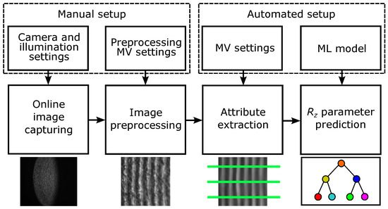
Figure 1. Steps of predicting the mounting hole roughness.

• Online capturing of images;
• Preprocessing of images;
• Extraction of attributes from the preprocessed images;
• Prediction of commutator mounting hole roughness based on the ML model.

A preparatory step in designing the online roughness prediction system was the selection of representative specimens. In addition, the roughness value of each specimen was measured to obtain the reference roughness values. These were later used to assess the prediction accuracy. A detailed description of each step of the proposed approach is presented in Section 3.1, Section 3.2, Section 3.3 and Section 3.4.

The parameter settings of image capturing and image preprocessing steps were determined by a domain expert, based on a trial-and-error method. The criterion in the online image capturing step was to find the camera-illumination setup, where the features of the commutator mounting hole surface were emphasized the most. In the image preprocessing step, the hole surface region was extracted from the original captured image. The MV operators were selected in a way that the MV algorithm always extracts the most informative region, regardless of its absolute position in the original image.

Extraction of attributes from an image and roughness prediction based on the extracted attributes are the crucial steps in designing the online roughness measurement system. The inputs are the MV algorithm settings and the ML model obtained during the optimization process in the development phase of the proposed system. In order to obtain the most appropriate MV and ML algorithm settings, the optimization procedure presented in Section 4 was carried out.

3.1. Data Preparation

The design of the online system for roughness measurements started with selecting representative samples and performing the reference roughness measurements. Surface roughness can be determined by several parameters that are categorized into amplitude parameters, spacing parameters, and hybrid parameters [22]. The commutator concerned in this study has a hole roughness defined by the parameter $R_z$; hence, this parameter was used as a roughness measure in the experiments. $R_z$ represents the height difference between the maximum peak height and the maximum valley depth of a line profile on a predetermined sampling length.

The samples were selected from a recalled batch of commutators with inadequate hole roughness values. The dataset contained 700 instances, which is significantly higher than the dataset in our initial study [5]. The dataset was split into the training set (630 instances) and hold-out set (70 instances) used for the result evaluation. The hold-out set was selected manually and represented 10% of all available instances. To achieve a representative distribution of instances with regard to the roughness parameter $R_z$, all 700 instances were sorted by the $R_z$ parameter value in ascending order and every tenth instance was moved to the hold-out set (systematic sampling).

The reference roughness measurements were performed by the contact profilometer Mitutoyo Surftest SJ-210. To reduce the measurement error originating from the previously described stylus sensitivity, the reference $R_z$ values were calculated as an average of three measurements. Commutators with the roughness parameter value $R_z\le$ 16 $\mathsf{\mu }$m are considered acceptable, while the ones with $R_z>$ 16 $\mathsf{\mu }$m unacceptable. The distribution of instances with regard to the $R_z$ value is shown in Figure 2.

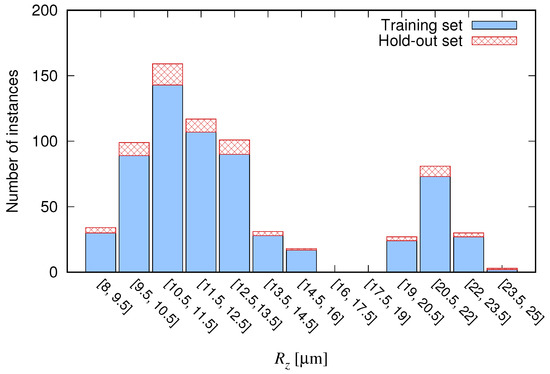
Figure 2. Distribution of instances with respect to the value of $R_z$.

3.2. Image Capturing and Preprocessing

The inner diameter of the commutator mounting hole concerned in this study is only 6 mm. This fact represented a major challenge in capturing the hole surface images. However, after the validation of several camera-illumination setups, the setup shown in Figure 3 was established.

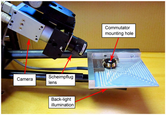
Figure 3. Camera-illumination setup.

Grayscale images of all 700 commutator mounting holes were manually captured and labeled with the corresponding reference roughness values. The 8-bit grayscale image of the mounting hole surface has a resolution of $2592\times 1944$ pixels. However, to be able to extract the attributes that are correlated with the $R_z$ roughness value, additional preprocessing of the images has to be performed. The purpose of preprocessing is to extract only the portion of the image where the hole surface treatment is clearly visible. The sequence of the MV operators used in the image preprocessing step is shown in Figure 4. The operators, their parameter settings and their sequence in the preprocessing step were determined based on the expert knowledge, gained in the development of similar MV applications.

Figure 4. Image preprocessing algorithm.

The initial step in preprocessing the images is binarization, where a binary threshold is applied to the 256-grayscale image. In the next step, the resulting binary image is used to calculate the image intensity centroid. Since the camera-illumination setup is designed in such a way that the hole surface image contains the highest proportion of high-intensity pixels, the calculated coordinates of intensity centroid are always positioned at about the same location of the mounting hole, regardless of its absolute position in the image. The coordinate system for precise positioning of an image mask is then applied to the calculated centroid position. Finally, the extraction mask positioned at the coordinate system origin is applied to the image, and the region of the mask size ($700\times 300$ pixels), i.e., the region of interest (ROI), is extracted from the original grayscale image. An example of the image with marked and extracted ROI can be seen in Figure 5.

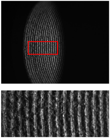
Figure 5. Captured image with marked ROI (top) and extracted part of the image (bottom).

3.3. Attribute Extraction

The attribute extraction algorithm consists of four image operators that require four parameters to be set. Similarly as in the image preprocessing, the operators and their sequence were determined manually, based on the expert knowledge and experience. The operators and their sequence in the attribute extraction algorithm are outlined in Figure 6.

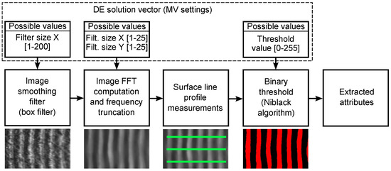
Figure 6. The attribute extraction algorithm.

First, a box filter with a varying kernel size $\{1,2,\dots ,200\}$ is applied to the image. Due to the inhomogeneities of the thermoset material used in commutator body manufacturing, some “salt-and-pepper” noise is present in the image. The box filter reduces this noise and emphasizes the features describing the mounting hole roughness. Next, the FFT filtering is applied, truncating a certain portion of high frequencies and thus additionally emphasizing the features that result from the machine treatment of the hole. The FFT filter enables to set the filter kernel size in both X and Y directions in the image, in the range of $\{1,2,\dots ,25\}$. Afterwarsd, line profile measurements analog to the contact profilometer measurements are performed on the grayscale image and the image attributes are extracted. An additional set of attributes is extracted after applying the Niblack binarization algorithm [23]. The threshold of the Niblack algorithm is set in the range of $\{1,2,\dots ,255\}$ and outputs a binary image consisting of the stripes representing the “peaks” and “valleys” on the commutator hole surface (see Figure 6).

In total, 24 numerical attributes describing the properties of the commutator mounting hole surface were extracted from each image. Specifically, 20 attributes were extracted from the grayscale images and four from the binary images. The grayscale attributes were describing the highest and the lowest grayscale value of a pixel in a selected line profile, the number of grayscale peaks and valleys along the line profile, and the mean grayscale value of all the peaks and valleys. In addition, four attributes representing the roughness parameter estimates were calculated from the grayscale line profile. These were $R_t$, $R_a$, and $R_z$ (ISO and DIN variants). Here, $R_t$ (maximum profile height) is determined as

$$R_t=r^{\max }-r^{\min },$$

(1)

where $r^{\max }$ is the highest grayscale value representing the highest peak and $r^{\min }$ the lowest grayscale value representing the lowest valley. $R_a$ (arithmetic mean of profile values) is calculated as

$$R_a=\frac{1}{n}\sum _1^n{r}_i,$$

(2)

where n is the number of values in the line profile and $r_i$ the i-th value in the profile. $R_z^{\mathrm{ISO}}$ is obtained as

$$R_z^{\mathrm{ISO}}=\frac{1}{5}\sum _{j=1}^5(r_j^{\max }-r_j^{\min }),$$

(3)

where $r_j^{\max }$ and $r_j^{\min }$ represent the highest peak and the lowest valley in the j-th profile, respectively. Similarly, $R_z^{\mathrm{DIN}}$ is determined as

$$R_z^{\mathrm{DIN}}=\frac{1}{N}\sum _{j=1}^N(r_j^{\max }-r_j^{\min }),$$

(4)

where N is the number of considered profiles. Details on these roughness parameters can be found in [3].

Moreover, the maximum, the minimum and the average peak and valley grayscale values were calculated. Lastly, two additional grayscale attributes, the maximum value of a grayscale image signal and its corresponding index, were extracted by the FFT algorithm. Finally, the four attributes extracted from the binary images were the percentage of pixels representing the peaks, the percentage of pixels representing the valleys, and the average peak and valley width in the image.

3.4. Roughness Prediction

The task in this research was to predict the value of the roughness parameter $R_z$ considering the attributes extracted from the images. An MV algorithm with given settings (Figure 6) was applied to the commutator mounting hole images to create a dataset of attributes. In the roughness prediction step, the ML predictive model was applied to the extracted attributes dataset, and the value of the roughness parameter $R_z$ is predicted. For $R_z$ prediction, algorithms for building regression trees and ensembles of regression trees were used. The reason for using the regression trees was in that they can be interpreted and their implementation in the online roughness measurement system is not overly complex.

Besides the MV parameter settings, the ML parameter settings influence the ML prediction accuracy too. In order to find suitable MV and ML algorithm settings, the optimization procedure presented in Section 4 was applied. The goal of this procedure was to find the ML model with the highest prediction accuracy.

The chosen evaluation metric was the root relative squared error (RRSE), which has already been used in [5]. It measures the error of the induced ML model in comparison to the error of a simple predictor which ignores the predictions and always outputs the average of the actual values. It is defined as

$$\mathrm{RRSE}=\sqrt{\frac{{\sum }_{i=1}^n{(p_i-a_i)}^2}{{\sum }_{i=1}^n{(a_i-\overline{a})}^2}}$$

(5)

where n is the number of instances, $p_i$ the predicted value of i-th instance, $a_i$ the actual value of i-th instance, and $\overline{a}$ the average actual value. The final results of the experiments were additionally assessed with respect to the mean absolute error

$$\mathrm{MAE}=\frac{1}{n}\sum _{i=1}^n|p_i-a_i|$$

(6)

that is informative for practical considerations as it is expressed in $\mathsf{\mu }$m.

4. Optimization of Algorithm Parameters

In contrast to manual search for suitable MV and ML algorithm parameter settings, the task can be formulated as an optimization problem where the goal is to find the MV and ML algorithm settings that minimize the roughness prediction error. The optimization procedure that produces the most accurate predictive model is shown in Figure 7.

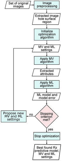
Figure 7. Optimization procedure that searches for the best MV and ML algorithm settings and outputs the best $R_z$ predictive model.

The input to the optimization procedure are images of the commutator mounting hole surfaces. First, the images are preprocessed to extract the part of the image where the mounting hole is located. During the first run of the optimization procedure, the initial MV and ML algorithm settings are set by the optimization algorithm. Based on these settings, the MV algorithm extracts the attributes from the images and creates an attribute file. The number of instances in the file corresponds to the number of input images. Next, the attribute file together with the previously initialized ML settings is passed to the ML algorithm. The output of the ML algorithm is a roughness predictive model and its objective function value, that is the RRSE prediction error. While the stopping criterion is not met, the optimization algorithm keeps generating new populations of solutions. The procedure of generating a new population depends on the employed optimization algorithm. In our case, solutions represent the MV and ML parameter settings, which are passed to the MV and ML algorithms and are in the next iteration evaluated by the optimization algorithm. The optimization procedure stops when a predefined number of solution evaluations is completed. The output of the optimization procedure is the best found roughness predictive model with the corresponding MV and ML algorithm parameter settings.

5. Experimental Setup and Validation Procedure

5.1. Setup

The software environment used in the experiments consisted of MV algorithms for image preprocessing and attribute extraction, the open-source data mining tool Weka [24], and the optimization algorithm jDE [25]. The components were integrated through an interface written in the C++ programming language.

The MV algorithms were implemented using the Open Computer Vision (OpenCV) library [26] and utilizing the CUDA parallel computing platform and programming module [27]. CUDA supports the use of graphical processing units (GPUs) for accelerated algorithm execution.

Weka was selected as a data mining tool since it is easy to call from the C++ interface. Two regression algorithms available in Weka were used to generate the roughness predictive models:

• M5P [28] for building regression trees, and
• RandomForest (RF) [29] for constructing forests of random trees.

Both algorithms involve various parameters that influence the training of predictive models and, consequently, the predictive model accuracy. In this study, the ML algorithm parameters were subject to an automated optimization procedure and, therefore, the best ML parameter values were found by the optimization algorithm.

The following parameters of the M5P algorithm and their values were considered in the optimization procedure:

• M, the minimum number of instances per leaf in the tree, $\{1,2,\dots ,20\}$;
• N, use of tree pruning, $\{true,false\}$;
• U, use of smoothing in predictions, $\{true,false\}$.

The parameters and their values for the RF algorithm were as follows:

• Depth, the maximum depth of the tree, $\{1,2,\dots ,150\}$;
• K, the number of attributes to randomly investigate, $\{1,2,\dots ,25\}$;
• I, the number of iterations, $\{20,21,\dots ,200\}$;
• B, randomly breaking the ties when several attributes are equally good, $\{true,false\}$.

The optimization algorithm jDE was used to search the MV and ML parameter decision spaces. jDE is a variant of differential evolution (DE) [6], where only the population size and the stopping condition need to be set manually, while the differential weight and the crossover rate are set through self-adaptation [25]. In all the experiments, the population size was set to 50 and 100 generations were examined, resulting in 5000 evaluated solutions per optimization run. The population size and the number of generations were determined empirically by monitoring the solution improvement over generations.

The decision space size in the case of optimizing the MV and M5P algorithm parameters was $2.6·{10}^9$ (number of possible MV and ML algorithm parameter settings, which is equal to the number of possible values multiplied over all parameters). In the case of optimizing the MV and RF algorithm parameters, it was even larger, i.e., $4.3·{10}^{13}$.

5.2. Validation Procedure

To build the most accurate roughness predictive model, the optimization was performed over the MV parameters, and the M5P and RF algorithm parameters. The optimization procedure was run ten times for each ML algorithm. Based on the extracted dataset of attributes, for each solution, namely ML and MV parameter settings, a regression predictive model was built. The prediction error, i.e., the RRSE value, of each built predictive model was calculated using 10-fold cross-validation (CV). This error was used as the predictive model accuracy estimate and was the optimization objective to be minimized. In Figure 8, the RRSE values averaged over ten optimization runs are denoted with suffix “OPT”. The error during the optimization runs could also be assessed using the hold-out set, but as shown in [30], in general, minimizing the error estimated with single CV also minimizes other error estimates.

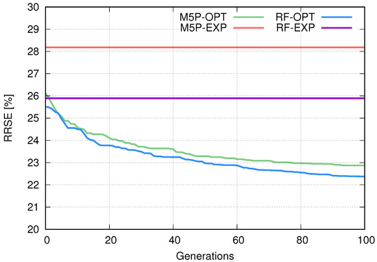
Figure 8. Roughness prediction error (RRSE) estimates for regression trees, random forests and the expert-defined setting. Error estimates for the optimized regression trees and random forests are averaged over ten runs and marked with suffix “OPT”. Error estimates for the expert defined setting are marked with “EXP”. For details see Section 5.2.

After each run of the optimization procedure, the accuracy of the best found predictive model was assessed using the hold-out set. In addition, the same RRSE assessment was performed for the M5P and RF predictive models built using the expert-defined MV settings. In this case, the expert settings were defined just for the MV parameters, while the parameters of the ML algorithms were set to their default values. Since a single predictive model is constructed in this way, the related result in Figure 8 is represented by a straight line and marked with the suffix “EXP”.

6. Results and Discussion

Observing the progress of optimization in terms of RRSE over generations for different algorithms and setups shown in Figure 8, one can draw several conclusions on the resulting predictive models and their accuracy.

First, the manual setup of the MV algorithm parameters does not result in optimal parameter settings. Comparison of the final RRSE values for the manual and optimized settings shows a major difference in the accuracy of the roughness predictive models. The results clearly show that the optimization of the MV parameter settings increases the prediction accuracy.

Next, using different ML algorithms results in predictive models of quite different prediction accuracy, i.e., average RRSE 28.2% for M5P and 25.9% for RF. Recall that the expert parameter settings of the MV algorithm in these runs were kept constant and the ML algorithm parameters were set to their default values. Given the fact that the default values of ML algorithm parameters are not optimized for a specific ML task, it can be expected that the optimization of the ML algorithm parameters improves the accuracy of the predictive model.

Finally, the comparison of the RRSE values averaged over the optimization runs for the M5P and RF algorithms shows that RF achieves better prediction results. In these runs, both the MV and ML algorithm parameters are subject to optimization. As a result, the average RRSE for M5P is 22.9% and for RF 22.4%.

Table 1 shows the comparison of the predictive models validation results between the expert and optimized MV parameters settings. The models were validated by 10-fold CV and by the hold-out set, and averaged over ten runs of each algorithm. The best average prediction accuracy was achieved by the “RF-OPT” algorithm. However, based on the comparison of the RRSE estimates for each ML algorithm, we can observe that the hold-out set validation always yields lower RRSE value than the 10-fold CV. This may be due to the performed systematic sampling of the instances in the hold-out set and relatively small size of the hold-out set (70 instances). The related MAE values were proportional to the RRSE results.

Table 1. Prediction error estimates.

Algorithm	10-Fold CV		Hold-Out Set
	RRSE [%]	MAE [$\mathsf{\mu }$m]	RRSE [%]	MAE [$\mathsf{\mu }$m]
M5P-EXP	28.2	0.82	26.1	0.84
RF-EXP	25.9	0.80	23.9	0.83
M5P-OPT	22.9	0.74	22.5	0.71
RF-OPT	22.4	0.71	21.9	0.70

To better understand the difference between the expert-defined MV settings and MV settings found by the optimization algorithm, we compared the MV algorithm output images. The differences between the original image and the images processed using the expert-defined and the jDE-optimized MV parameter settings are shown in Figure 9. The images processed using the expert-defined and the jDE-optimized MV settings are in comparison to the original image filtered and smoothed. They are very similar from the human eye perspective. However, based on the differences in the output image, a predictive model with a substantially better prediction accuracy is built in the latter case. This indicates that even small differences in image preprocessing arising from different MV parameter settings can result in improved prediction accuracy.

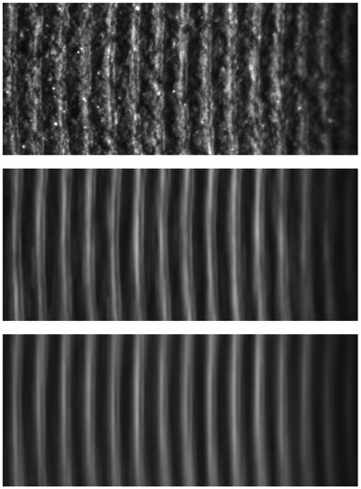
Figure 9. Comparison of the processed images using the expert and the optimized settings: the original extracted image (top), the image processed with expert-defined MV parameter settings (center), and the image processed with MV and ML parameters set by the optimization algorithm (bottom).

In addition, we analyzed the most informative attributes appearing in the predictive models. The analysis was performed in Weka [24] for the M5P and RF algorithms. The most informative attributes were always selected from the grayscale image attributes mostly describing the geometrical properties of the commutator mounting hole. These properties result from the final treatment of the commutator mounting hole. Regardless of the used ML algorithm, the five most frequent attributes were the number of detected valleys in the image, the number of detected peaks in the image, the lowest grayscale value of a pixel in the valley, and the minimum and the average valley width. Recall that the roughness parameter $R_z$, which we are trying to predict, represents the maximum difference between the peak height and the valley depth along the measured line profile. Based on this knowledge, the connection between the geometrical properties extracted from the image and the $R_z$ parameter can be interpreted. However, other attributes were also used to build the predictive models, but their selection varied depending on the used algorithm and specific run.

To verify the prediction results of the M5P and RF algorithms using the optimized settings, the best model found by each algorithm was identified and applied to predict the roughness of all 700 instances. This was done separately for the training set and the hold-out set. The results of prediction for the two learning algorithms are shown in Figure 10 and Figure 11, respectively.

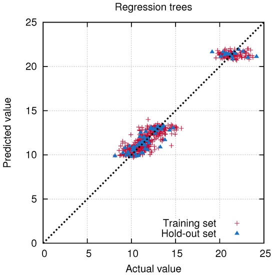
Figure 10. Comparison of the measured and predicted values of $R_z$ for the training and hold-out set, using the best found regression tree model.

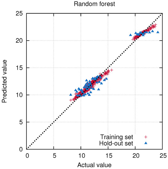
Figure 11. Comparison of the measured and predicted values of $R_z$ for the training and hold-out sets, using the best found random forest model.

The results of the M5P regression tree show that the accuracies on the training set and the hold-out set are similar. The estimated RRSE of the best regression tree found on the training set was 21.2%, while the RSSE achieved on the hold-out set was 22.5%. The MAE of this predictive model assessed on the hold-out set was 0.71 $\mathsf{\mu }$m, which is an acceptable result for practical application.

Comparison of the prediction accuracy of the M5P and RF models shows that the spread of prediction error is much lower in the case of RF. The best found RF model has the RRSE measured on the training set equal to 8.6%, while the estimated RRSE of the same model on the hold-out set is 22.1%. The MAE of this model assessed on the hold-out set is 0.70 $\mathsf{\mu }$m.

In addition, we compared the accuracy of the best found predictive model and the accuracy of the existing contact method. Recall that the reference value of the roughness parameter $R_z$ was calculated as an average of three measurements performed with a contact profilometer. The MAE of these measurements was calculated as a difference between a randomly selected one of the three measurements and the average value of these three measurements. The resulting value was 0.60 $\mathsf{\mu }$m. The MAE of the best RF model was 0.70 $\mathsf{\mu }$m, which is comparable to the accuracy of the contact measurements. In addition, it was confirmed by a customer that the method is appropriate to perform the statistical process control (SPC) in the commutator production.

The proposed MV-based roughness measurement method has, in comparison to the existing contact method, several advantages. Performing a single measurement with a contact profilometer takes at least 10 seconds, while a complete MV-based measurement, which consists of capturing the image, extracting the attributes and predicting the roughness value, is performed in approximately one second. Since the MV-based method is very efficient and enables contactless measurements, it is suitable for online implementation. In addition, if the method is used in SPC, it enables to perform a higher number of roughness measurements per batch, resulting in a higher reliability of SPC.

7. Conclusions

This paper presents a novel method of measuring the surface roughness of specific machined parts for the automotive industry. The method is based on the MV quality control that enables online and real-time roughness measurements. In addition to MV, the methodology combines ML and evolutionary optimization to build an accurate model for predicting the $R_z$ roughness parameter. The evolutionary optimization algorithm searches for appropriate MV and ML parameter settings to produce a predictive model of acceptable accuracy.

During the development of the MV-based roughness measurement system, two ML algorithms were tested: an algorithm for building the regression trees and a random forest algorithm. The random forest algorithm proved to be more repeatable and accurate on average than the regression tree algorithm; however, the best solutions found by both algorithms were comparable. During the MV and ML parameter optimization, the prediction error was assessed by 10-fold cross-validation. After the optimization, the accuracy of the final predictive models was tested on a hold-out set of previously unseen instances. The validation showed that the found predictive models achieved comparable accuracy on training and hold-out datasets. In addition, it was confirmed, that the optimization methodology is beneficial in setting of the MV parameters for reliable quality control.

The best found RF predictive model has the RRSE value of 22.1%, resulting in the absolute mean prediction error of 0.70 $\mathsf{\mu }$m. This result is satisfactory and comparable to the accuracy of the SPC contact roughness measurement systems currently installed in the commutator production. However, the developed methodology enables to perform the roughness measurement on the production line and control the quality of the turning process online and in real-time.

The optimization methodology presented in this work can be applied to any MV algorithm to tune its settings and build a predictive model. Nonetheless, the MV operators and their sequence used in the optimization procedure were determined manually, relying on the expert knowledge and experience. Therefore, they may not be optimally selected, and consequently, the prediction error of the best found regression model, in the case of using alternative MV operators and their sequence, could be even lower. Accordingly, our future work will focus on upgrading the presented methodology with automated MV algorithm construction where expert assistance will no longer be needed.

References

- Hamed, A.M.; Saudy, M. Computation of surface roughness using optical correlation. Pramana 2007, 68, 831–842. [Google Scholar] [CrossRef]
- Thomas, T. Rough Surfaces; Imperial College Press: London, UK, 1999. [Google Scholar] [CrossRef]
- Whitehouse, D.J. Handbook of Surface and Nanometrology; CRC Press: Boca Raton, FL, USA, 2010. [Google Scholar] [CrossRef]
- Blunt, L.; Jiang, X. (Eds.) Advanced Techniques for Assessment Surface Topography: Development of a Basis for 3D Surface Texture Standards “Surfstand”; Butterworth-Heinemann: Oxford, UK, 2003. [Google Scholar] [CrossRef]
- Koblar, V.; Pečar, M.; Gantar, K.; Tušar, T.; Filipič, B. Determining surface roughness of semifinished products using computer vision and machine learning. In Proceedings of the 18th International Multiconference Information Society (IS 2015), Ljubljana, Slovenia, 28 September–14 October 2015; Volume A, pp. 51–54. [Google Scholar]
- Storn, R.; Price, K. Differential evolution: A simple and efficient heuristic for global optimization over continuous spaces. J. Glob. Optim. 1997, 11, 341–359. [Google Scholar] [CrossRef]
- Shahabi, H.H.; Ratnam, M.M. Noncontact roughness measurement of turned parts using machine vision. Int. J. Adv. Manuf. Technol. 2010, 46, 275–284. [Google Scholar] [CrossRef]
- Jeyapoovan, M.T.; Murugan, M. Surface roughness classfication using image processing. Measurement 2013, 46, 2065–2072. [Google Scholar] [CrossRef]
- Nithyanantham, N.; Suresh, P. Evaluation of cast iron surface roughness using image processing and machine vision system. ARPN J. Eng. Appl. Sci. 2016, 11, 1111–1116. [Google Scholar]
- Jibin, G.J.; Arunachalam, N. Illumination compensated images for surface roughness evaluation using machine vision in grinding process. Procedia Manuf. 2019, 34, 969–977. [Google Scholar] [CrossRef]
- Patel, D.R.P.; Kiran, M. Vision based prediction of surface roughness for end milling. Mater. Today Proc. 2020, 44, 792–796. [Google Scholar] [CrossRef]
- Fadare, D.A.; Oni, A.O. Development and application of a machine vision system for measurement of surface roughness. ARPN J. Eng. Appl. Sci. 2009, 4, 30–37. [Google Scholar]
- Ravikumar, S.; Ramachandran, K.I.; Sugumaran, V. Machine learning approach for automated visual inspection of machine components. Expert Syst. Appl. 2011, 38, 3260–3266. [Google Scholar] [CrossRef]
- Samtaş, G. Measurement and evaluation of surface roughness based on optic system using image processing and artificial neural network. Int. J. Adv. Manuf. Technol. 2014, 73, 353–364. [Google Scholar] [CrossRef]
- Elangovan, M.; Sakthivel, N.; Saravanamurugan, S.; Nair, B.; Sugumaran, V. Machine learning approach to the prediction of surface roughness using statistical features of vibration signal acquired in turning. Procedia Comput. Sci. 2015, 50, 282–288. [Google Scholar] [CrossRef]
- Simunovic, G.; Svalina, I.; Simunovic, K.; Saric, T.; Havrlisan, S.; Vukelic, D. Surface roughness assessing based on digital image features. Adv. Prod. Eng. Manag. 2016, 11, 93–104. [Google Scholar] [CrossRef][Green Version]
- Yi, H.; Liu, J.; Ao, P.; Lu, E.; Zhang, H. Visual method for measuring the roughness of a grinding piece based on color indices. Opt. Express 2016, 24, 17215–17233. [Google Scholar] [CrossRef] [PubMed]
- Morales Tamayo, Y.; Beltrán Reyna, R.F.; López Bustamante, R.J.; Zamora Hernández, Y.; López Cedeño, K.; Terán Herrera, H.C. Comparison of two methods for predicting surface roughness in turning stainless steel AISI 316L. Ingeniare. Revista Chilena de Ingeniería 2018, 26, 97–105. [Google Scholar] [CrossRef]
- Lin, Y.C.; Wu, K.D.; Shih, W.C.; Hsu, P.K.; Hung, J.P. Prediction of surface roughness based on cutting parameters and machining vibration in end milling using regression method and artificial neural network. Appl. Sci. 2020, 10, 3941. [Google Scholar] [CrossRef]
- Reris, R.; Brooks, J.P. Principal component analysis and optimization: A tutorial. In Proceedings of the 14th INFORMS Computing Society Conference, Richmond, VA, USA, 11–13 January 2015; pp. 212–225. [Google Scholar]
- Grinblat, G.L.; Uzal, L.C.; Verdes, P.F.; Granitto, P.M. Nonstationary regression with support vector machines. Neural Comput. Appl. 2015, 26, 641–649. [Google Scholar] [CrossRef]
- Gadelmawla, E.; Koura, M.; Maksoud, T.; Elewa, I.; Soliman, H. Roughness parameters. J. Mater. Process. Technol. 2002, 123, 133–145. [Google Scholar] [CrossRef]
- Trier, O.D.; Jain, A.K. Goal-directed evaluation of binarization methods. IEEE Trans. Pattern Anal. Mach. Intell. 1995, 17, 1191–1201. [Google Scholar] [CrossRef]
- Hall, M.; Frank, E.; Holmes, G.; Pfahringer, B.; Reutemann, P.; Witten, I.H. The WEKA data mining software: An update. ACM SIGKDD Explor. Newsl. 2009, 11, 10–18. [Google Scholar] [CrossRef]
- Brest, J.; Greiner, S.; Bošković, B.; Mernik, M.; Žumer, V. Self-adapting control parameters in differential evolution: A comparative study on numerical benchmark problems. IEEE Trans. Evolut. Comput. 2006, 10, 646–657. [Google Scholar] [CrossRef]
- OpenCV: Open Source Computer Vision. Available online: https://opencv.org/ (accessed on 5 June 2018).
- NVIDIA. CUDA: Parallel Computing Platform and Programming Model. Available online: https://developer.nvidia.com/cuda-zone/ (accessed on 14 May 2018).
- Wang, Y.; Witten, I.H. Inducing model trees for continuous classes. In Proceedings of the 9th European Conference on Machine Learning, Prague, Czech Republic, 23–25 April 1997; pp. 128–137. [Google Scholar]
- Breiman, L. Random Forests. Mach. Learn. 2001, 45, 5–32. [Google Scholar] [CrossRef]
- Tušar, T.; Gantar, K.; Koblar, V.; Ženko, B.; Filipič, B. A study of overfitting in optimization of a manufacturing quality control procedure. Appl. Soft Comput. 2017, 59, 77–87. [Google Scholar] [CrossRef]
Publisher’s Note: MDPI stays neutral with regard to jurisdictional claims in published maps and institutional affiliations. |
© 2021 by the authors. Licensee MDPI, Basel, Switzerland. This article is an open access article distributed under the terms and conditions of the Creative Commons Attribution (CC BY) license (https://creativecommons.org/licenses/by/4.0/).