Abstract
State space model representation is widely used for the estimation of nonobservable (hidden) random variables when noisy observations of the associated stochastic process are available. In case the state vector is subject to constraints, the standard Kalman filtering algorithm can no longer be used in the estimation procedure, since it assumes the linearity of the model. This kind of issue is considered in what follows for the case of hidden variables that have to be non-negative. This restriction, which is common in many real applications, can be faced by describing the dynamic system of the hidden variables through non-negative definite quadratic forms. Such a model could describe any process where a positive component represents “gain”, while the negative one represents “loss”; the observation is derived from the difference between the two components, which stands for the “surplus”. Here, a thorough analysis of the conditions that have to be satisfied regarding the existence of non-negative estimations of the hidden variables is presented via the use of the Karush–Kuhn–Tucker conditions.
1. Introduction
State space modeling is used for estimating—revealing the dynamic evolution of hidden variables’ processes. In some cases, the state vector, which includes the hidden components, is subject to constraints, which are derived either due to the physical meaning of the states or because of the mathematical properties that have to be satisfied. For example, state space models with constraints are used in camera surveillance [1,2], navigation issues [3], and biological systems [4]. Especially, in finance, the hidden variables are often subject to non-negative constraints or in general have to be bounded. For example, in the Vasicek model [5] and its extension [6], the interest rates are considered to be hidden random variables subject to non-negative constraints, while in [7,8], the eigenvalues of the VAR process were restricted within the unit circle. Considering the use of state space models in the domain of finance, a discrete state space model could be implemented for the estimation of the hidden jump components of asset returns [9,10]. The use of jumps has been proposed for the description of the dynamics of asset prices since they can explain some of the empirical characteristics of the asset prices, e.g., the lack of a normal distribution or the existence of leptokurticity (see for example [11]).
When dealing with state space models that are subject to constraints, the Kalman filtering algorithm [12] can no longer be used, since it assumes linearity in the model. In the domain of nonlinear filters, the particle filtering approach (see for example [13,14,15,16]) has wide applicability, and it adopts resampling techniques for the estimation of the state vector at every time t. However, the use of resampling techniques adds considerable computational cost in the estimation procedure.
In this work, the observation is defined as the difference between the two-sided components under noise inclusion. The components are considered to be hidden random variables, and therefore, a state space model is established, where the state equation describes the dynamic evolution of the two hidden components. This equation represents a first-order Markov process, i.e., all the information needed for the estimation of the components at time t is derived by the components at time , and no other information from past times is needed. Moreover, the state vector is subject to non-negative constraints that have to be taken into account for its estimation in time. Such a model could describe, for example, the evolution of a system where the positive component represents “gain”, while the negative one represents “loss”; the observation is derives from the difference between the two components, which stands for the “surplus”, under noise inclusion. In asset pricing, an asset return can be defined as the difference between the two-sided non-negative return jump components under noise inclusion, and the jump components are considered to be hidden variables. Another example could be the one-dimensional random walk, where a positive jump could represent (the measure of) a move to the right and a negative jump (the measure of) a move to the left, while the observation could be a function of the two jump components given at discrete times. To handle such kinds of problems, non-negative definite quadratic forms are adopted in the state equation for the dynamic evolution of the two-sided components. In this case, the recursive equations of the Kalman filter cannot be used for the estimation of the state vector, since this filter assumes linearity in the measurement and state equation. To this end, this work first derives the recursive equations for the estimation of the state vector based on the state space model representation with non-negative definite quadratic forms in the state equation and their Taylor expansions. Then, a thorough analysis of the necessary conditions that have to be satisfied in order to obtain the non-negative estimations at every time t is provided. In Proposition 1, the stationary points of the optimization problem with the non-negative constraints are given by using the Karush–Kuhn–Tucker conditions, while in Proposition 2, the necessary conditions for the existence of feasible solutions in the constrained optimization problem are provided.
Overall, this work proposes a method in state space modeling representation, which can be used when dealing with hidden components that are subject to non-negativity constraints. The method results in the formulation of a constrained optimization problem for which the stationary points are derived via Proposition 1, and the necessary conditions for the existence of feasible solutions in this optimization problem are provided via Proposition 2; to that end, the iterative formulas for the minimum variance a posteriori estimators for the (hidden) state vector are illustrated. Moreover, the proposed method has a low computational burden compared to other nonlinear filtering methods that can be used in state space modeling with inequality constraints and are based on resampling techniques (e.g., particle filtering).
The paper is organized as follows. In Section 2, the state space model proposed for the estimation of the two jump components is established. Two non-negative quadratic forms are adopted to describe the dynamic evolution of the two-sided components subject to their non-negative restrictions. In Section 3, the recursive equations of the second-order Kalman filter are presented, while in Section 4, a thorough analysis of the conditions that have to be fulfilled so as to have non-negative estimations is presented. The results of this analysis are summarized in Propositions 1 and 2. In Section 5, an illustrative example concerning the evolution of positive and negative jumps of asset returns is presented to demonstrate the theoretical results. Finally, Section 6 concludes on the findings and provides suggestions for future work.
2. State Space Model
In this section, a state space model representation is illustrated considering the case where there are two hidden processes subject to non-negativity constraints. The state equation that describes the dynamic evolution of the hidden components adopts the use of non-negative definite quadratic forms, while the measurement equation is linear.
The state equation is given by:
or equivalently:
where:
- stands for the state vector;
- stands for the noise, and it is assumed that , where ;
- , is a (symmetric, ) non-negative definite matrix, i.e.,
The vector is a () column vector, where the k-th element equals 1, and the other element equals 0. The measurement equation is given by the relation:
where H = and . Moreover, it is assumed that .
Apparently, state Equation (2) describes a (nonobservable) first-order non-negative valued Markovian process, the evolution of which and its characteristics (e.g., periodicity, convergence etc.) depend on the structure (values) of the associated noisy observation sequence. The aim of our study here was to estimate (reveal) the Markovian process (2) (i.e., the matrices , and ), through the observation Equation (3), if the components of the state vector have to be non-negative. For this purpose, Model (2) and (3) adopts the use of non-negative definite quadratic forms to describe the dynamic evolution of the hidden two-sided components; that is, to ensure that the estimations of the components will be non-negative. To that end, the extended Kalman filter of second order is proposed in order to estimate at every time t the state vector that incorporates the hidden jump components. It is noticed here that the noise component in Relation (2) is multiplicative and not additive.
Next, the extended Kalman filter of second order is described and its iterative equations for the estimation of the state vector are presented.
3. Extended Kalman Filter of Second Order
Model (2) and (3) presented in Section 2 is nonlinear, and subsequently, the recursive standard algorithm of the Kalman filter cannot be used for the estimation of the state vector. Aiming to derive the recursive equations for the estimation of the hidden states taking into consideration that the state Equation (2) is a quadratic form, the following notation is used:
- : the a priori estimation of the state vector , i.e., without taking into consideration the measurement at time t;
- : the a posteriori estimation of the state vector , i.e., by considering the measurement at time t;
- , : the variance–covariance matrices of the a priori and a posteriori error estimations of , respectively, i.e.,
According to (2), , is a function of the random variables , and , i.e., . Then, using the Taylor expansion of second order of at , it is derived that:
where functions , , are given in (1). By equating the mean values in Relation (4), the a priori estimation of (prediction stage) is derived, that is:
and the entries of the respective variance–covariance matrix are given by the relation,
where denotes the -element of matrix and denotes the trace of the respective matrix. Taking into consideration the properties of the trace of a matrix, it is derived after some algebraic manipulations on Relations (5) and (6) that:
Regarding the a posteriori estimations of , it is taken into account that the joint distribution of and is normal, based on the relation:
Then, we make use of the following Lemma (see for example [17]):
Lemma 1.
Let , be two random variables that are jointly normally distributed with:
Then, , where:
Based on Lemma 1, the a posteriori estimation of (update stage) and the related variance–covariance matrix are given by,
where . By using the recursive Relations (7)–(10), we can estimate the hidden components at every time t.
Next, a detailed investigation regarding the existence of non-negative solutions (i.e., non-negative a posteriori estimations of ) derived from (9) is presented.
4. Investigation of the State Space Model
In what follows, we present an investigation concerning the conditions that have to be satisfied so as to derive non-negative a posteriori estimations of the state vector . Obviously, Relation (7) ensures the existence of non-negative a priori estimations of at every time t. However, the a posteriori estimations of given by (9) may not fulfil the non-negativity condition. We note that the solutions depend on the term , the sign of which is not time invariant. To this end, in order to ensure that the a posteriori unbiased estimator will be a minimum variance estimator under the non-negativity restrictions that its components must satisfy, the following optimization problem arises,
Symbol ⪰ (or ⪯) is used for the elementwise inequality, while is given by Equation (1) (or (2)). The following Proposition 1 provides the set of stationary points related to the optimization problem (11), subject to the non-negativity restrictions. This set includes the optimal solution, i.e., the unbiased minimum variance estimator . In what follows, we use the following notations:
.
Remark 1.
Notice that, if , then Relation (9) leads to , and consequently, the solution is acceptable.
Taking into consideration Remark 1, it is assumed in the sequel that for every t.
Proposition 1.
The weight matrix and the stationary points related to the optimization problem (11) are given by the relations:
- (i)
- , which leads to the solution:
- (ii)
- which leads to the solution:and:
- (iii)
- , which leads to the solution:and:
- (iv)
- , which leads to the solution:where denotes the -row of matrix , .
Proof.
The Lagrangian function related to the optimization problem (11) is defined as:
Based on (10), it is derived that:
while (by assuming the dependence of on and , , as provided in Kalman filtering):
By calculating the first derivative of the Lagrangian function and equating it to 0, it is derived that:
where . Thus, matrix has to satisfy the following condition (by noticing that is symmetric):
based on the constraints [18]:
.
The following cases have to be considered:
- (i)
- The two constraint conditions are inactive. Then, , and the optimization problem, leading to (14), is transformed into the unconstrained one considered in the case of the Kalman filter. It is derived that:which is the well-known Kalman gain matrix. The related solution in terms of the a posteriori estimator is:Relation (16) constitutes a possible solution of the optimization problem (11), and it has to satisfy the constraint ;
- (ii)
- The first constraint condition is inactive (i.e., ), while the second one is active. Then, the following two cases are considered:
- (a)
- If , then we are led to the unconstrained optimization problem presented in Case (i), and the solution must satisfy the non-negative restrictions, i.e.,
- (b)
- (iii)
- The first constraint condition is active, while the second one is inactive (i.e., ). The following two cases are considered:
- (a)
- If , then we obtain the unconstrained optimization problem presented in Case (i), and the solution must fulfil the nonnegative restrictions, i.e., ;
- (b)
- (iv)
- The two constraint conditions are active, i.e., and . In this case, we have to seek solutions such that , .
Based on the active constraint conditions, it is derived that:
i.e., , resulting in the relation,
The state vector constitutes a feasible solution, and it has to be checked whether Relation (14) is satisfied with , . □
In what follows, Proposition 2 provides the necessary conditions for the existence of feasible solutions regarding the constrained filter.
Proposition 2.
The solutions given in Proposition 1 regarding the optimization problem (11) are feasible upon the following conditions (necessary conditions):
- (i)
- constitutes a feasible solution, if:
- (ii)
- constitutes a feasible solution, if:and:
- (iii)
- constitutes a feasible solution, if:and:
- (iv)
- constitutes a feasible solution, if:and:
Proof.
Similar to the proof of Proposition 1, four cases are considered:
- (i)
- The two constraint conditions are inactive. Then, , and the optimization problem is transformed into the unconstrained one that is met in the case of the Kalman filter. In this case, based on Proposition 1, we obtain that , resulting in the estimation:where is a feasible solution of the optimization problem with the nonnegative constraints, if:Consequently, the necessary condition is formulated as follows:
- (ii)
- The first constraint condition is inactive, while the second one is active, i.e, and , respectively. The following two cases are considered:
- (a)
- (b)
- If , matrix has to be in such a form so that .It is derived via the active constraint condition that where based on Remark 1. Then, (14) results in:
- (iii)
- The first constraint condition is active, while the second one is inactive, i.e., and , respectively. The following two cases are considered:
- (a)
- and ;
- (b)
- and .
Similar to Case (ii), the third part of Proposition 2 can be derived; - (iv)
- The two constraint conditions are active, i.e., and . In this case, we have to search for solutions where . It is derived via Proposition 1 that:which leads to the solution .The following subcases are considered:
- (a)
- (b)
- If and , then by taking into consideration Case (iib), it is concluded that the solution is accepted, if:Otherwise, it is rejected since it is not aligned with the conditions of the considered case (i.e., );
- (c)
- If and , similar to Case (iv)-c, the solution is accepted, if:
- (d)
In conclusion, in Case (iv), the vector is a possible optimal solution, if at least one of the following conditions holds:
. □
Remark 2.
Based on the low computational cost, the four possible solutions of the constrained optimization problem (11) can be examined one-to-one, aiming to find the optimal solution. In any case, the necessary conditions presented in Proposition 2 can be examined simultaneously to have a more comprehensive view in the process of searching for the optimal solution.
Next, an illustrative application of the described methodology is presented regarding the estimation (revelation) of the two-sided jump components of asset returns.
5. Application; Estimation of the Two-Sided Jump Components of the NASDAQ Index
In this section, an application example of the proposed methodology analyzed in Section 4 is illustrated concerning the estimation of the hidden two-sided jump components of the NASDAQ index for the 3 y period 2006–2008. To estimate the parameters of the model, i.e., the parameter set , the maximum likelihood estimation method is used taking into consideration that the distribution of conditioned on is normal, i.e.,
Therefore, the log-likelihood function, LogL, is of the form:
where,
The estimations derived by maximizing , given in (26), are as follows:
and:
with = 995.9854. Based on the estimated parameters, the estimated two-sided jump components of the NASDAQ index are showcased in Figure 1.
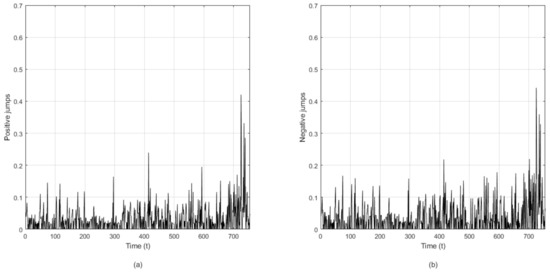
Figure 1.
(a) Estimated positive return jumps of the NASDAQ index during 2006–2008. (b) Estimated negative return jumps of the NASDAQ index during 2006–2008.
6. Conclusions
In this work, the topic of state space modeling with non-negative constraints was considered. For that purpose, a state space model was constructed where the state equation that describes the dynamic evolution of the components of the hidden state vector was expressed via non-negative definite quadratic forms and represents a non-negative valued Markovian stochastic process of order one. Due to the inequality conditions, a constrained optimization problem arises to derive estimators for the states, which are unbiased and of minimum variance. Towards this direction, a thorough analysis was illustrated via Propositions 1 and 2, concerning the stationary points of the optimization problem along with the special conditions that have to be satisfied in order to derive non-negative estimations for the state vectors at every time. Thus, in Proposition 2, necessary conditions were derived for a stationary point to constitute a feasible solution. The proposed method constitutes an alternative for handling state space models with non-negativity constraints, and it has a low computational burden compared to resampling methods for the estimation procedure.
Regarding future work, the generalization of the proposed method for the case of an n-dimensional non-negative state vector, , could be examined. This is a challenging problem in many applications. For example, in navigation problems, for , state space models with non-negativity constraints are suitable to describe the distance covered during the motion of a vehicle, if we let the three non-negative components of the state vector represent the measures of the velocities (speeds) along the axes in .
Author Contributions
Methodology, O.T. and G.T.; Writing—original draft, O.T. and G.T.; Writing—review & editing, O.T. and G.T. Both authors have read and agreed to the published version of the manuscript.
Funding
This research received no external funding.
Institutional Review Board Statement
Not applicable.
Informed Consent Statement
Not applicable.
Data Availability Statement
The dataset used to illustrate the applicability of the proposed method is publicly available at www.finance.yahoo.com accessed on 11 June 2021.
Conflicts of Interest
The authors declare no conflict of interest.
References
- Julier, S.; LaViola, J. On kalman filtering with nonlinear equality constraints. IEEE Trans. Signal Process. 2007, 55, 2774–2784. [Google Scholar] [CrossRef] [Green Version]
- Loumponias, K.; Vretos, N.; Tsaklidis, G.; Daras, P. An Improved Tobit Kalman Filter with Adaptive Censoring Limits. Circuits Syst. Signal Process. 2020, 39, 5588–5617. [Google Scholar] [CrossRef]
- Wang, L.; Chiang, Y.; Chang, F. Filtering method for nonlinear systems with constraints. Control. Theory Appl. IEE Proc. 2002, 149, 525–531. [Google Scholar] [CrossRef]
- Chia, T.; Chow, P.; Chizeck, H. Recursive parameter identification of constrained systems: An application to electrically stimulated muscle. IEEE Trans. Biomed. Eng. 1991, 38, 429–442. [Google Scholar] [CrossRef] [PubMed]
- Vasicek, O. An equilibrium characterization of the term structure. J. Financ. Econ. 1997, 5, 177–188. [Google Scholar] [CrossRef]
- Hull, J.; White, A. Pricing interest rate derivatives. Rev. Financ. Stud. 1990, 3, 573–592. [Google Scholar] [CrossRef]
- Cogleya, T.; Sargent, T. Drifts and volatilities: Monetary policies and outcomes in the post WWII US. Rev. Econ. Dyn. 2005, 8, 262–302. [Google Scholar] [CrossRef] [Green Version]
- Cogley, T.; Sargent, T. Evolving post World War II US inflation dynamics. Nber Macroecon. Annu. 2001, 16, 331–373. [Google Scholar] [CrossRef]
- Theodosiadou, O.; Tsaklidis, G. Estimating the Positive and Negative Jumps of Asset Returns via Kalman Filtering: The Case of NASDAQ Index. J. Methodol. Comput. Appl. Probab. 2017, 19, 1123–1134. [Google Scholar] [CrossRef]
- Theodosiadou, O.; Skaperas, S.; Tsaklidis, G. Change Point Detection and Estimation of the Two-Sided Jumps of Asset Returns using a Modified Kalman Filter. J. Risks 2017, 5, 15. [Google Scholar] [CrossRef] [Green Version]
- Cont, R. Empirical properties of asset returns: Stylized facts and statistical issues. Quant. Financ. 2001, 1, 223–236. [Google Scholar] [CrossRef]
- Kalman, R. A new approach to linear filtering and prediction problems. J. Basic Eng. Trans. ASME Ser. 1960, 82, 35–45. [Google Scholar] [CrossRef] [Green Version]
- Gordon, N.; Salmond, D.; Smith, A. Novel Approach to Nonlinear/Non-Gaussian Bayesian State Estimation. Radar Signal Process. IEE Proc. F 1993, 140, 107–113. [Google Scholar] [CrossRef] [Green Version]
- Doucet, A.; Johansen, A. A Tutorial on Particle Filtering and Smoothing: Fifteen years later. In Handbook of Nonlinear Filtering; Oxford University Press: Oxford, UK, 2008. [Google Scholar]
- Doucet, A.; de Freitas, N.; Gordon, N. (Eds.) Sequential Monte Carlo Methods in Practice; Springer: New York, NY, USA, 2001. [Google Scholar]
- Urteaga, I.; Bugallo, M.F.; Djurić, P.M. Sequential Monte Carlo methods under model uncertainty. In Proceedings of the 2016 IEEE Statistical Signal Processing Workshop (SSP), Palma de Mallorca, Spain, 26–29 June 2016; pp. 1–5. [Google Scholar]
- Kotz, S.; Balakrinshnan, N.; Johnson, N. Continouous Multivariate Distributions; Wiley: New York, NY, USA, 1995; Volume 1. [Google Scholar]
- Griva, I.; Nash, S.; Sofer, A. Linear and Nonlinear Optimization, 3rd ed.; SIAM: Philadelphia, PA, USA, 2008. [Google Scholar]

Publisher’s Note: MDPI stays neutral with regard to jurisdictional claims in published maps and institutional affiliations. |
© 2021 by the authors. Licensee MDPI, Basel, Switzerland. This article is an open access article distributed under the terms and conditions of the Creative Commons Attribution (CC BY) license (https://creativecommons.org/licenses/by/4.0/).