
An Extension of the Truncated-Exponential Skew- Normal Distribution


 ,
,  ,
,  and
and 
Abstract
:1. Introduction
2. Incorporating Kurtosis
2.1. Representation
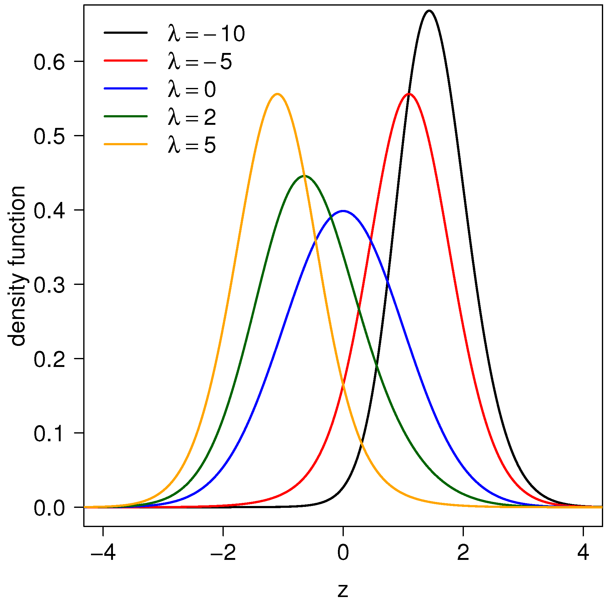
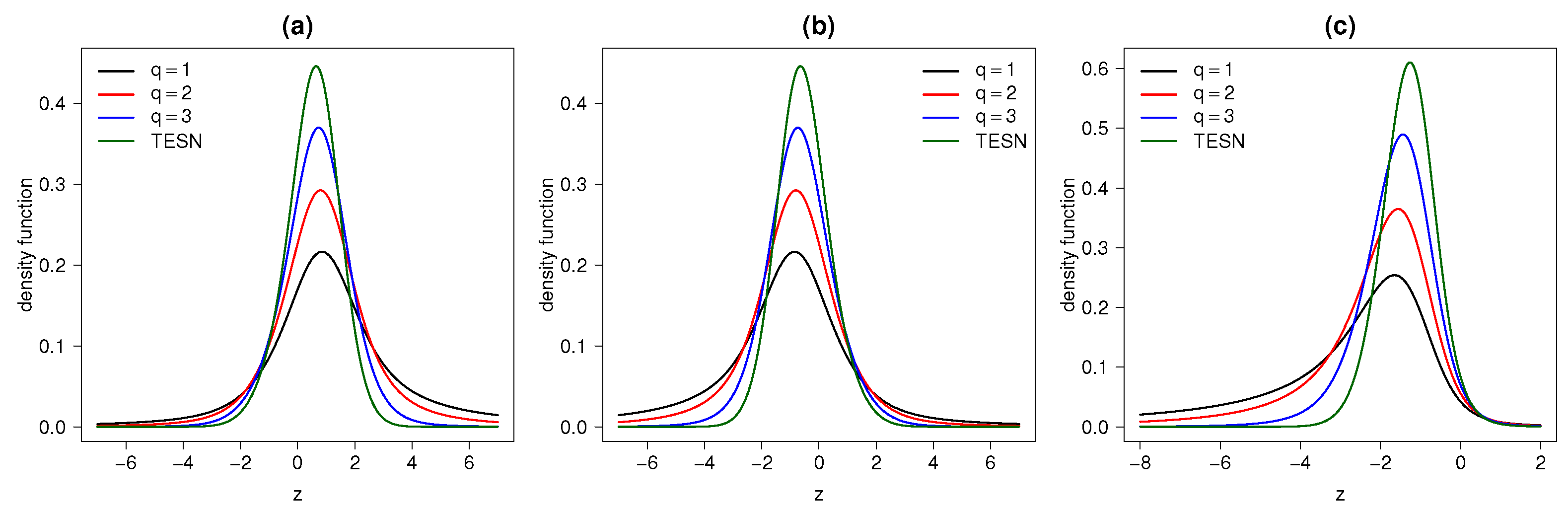
2.2. Probability Density Function
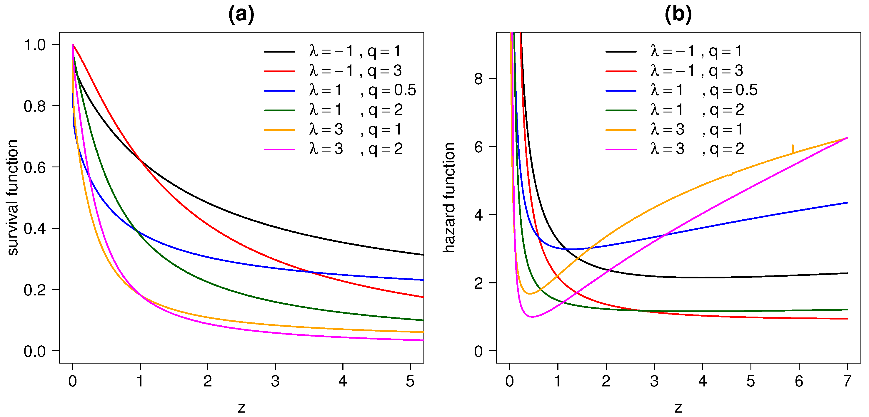
2.3. Reliability Analysis
2.4. Moments
2.5. Incorporation of Parameters
2.6. Log Likelihood Equations
2.7. STESN or TESN Model?
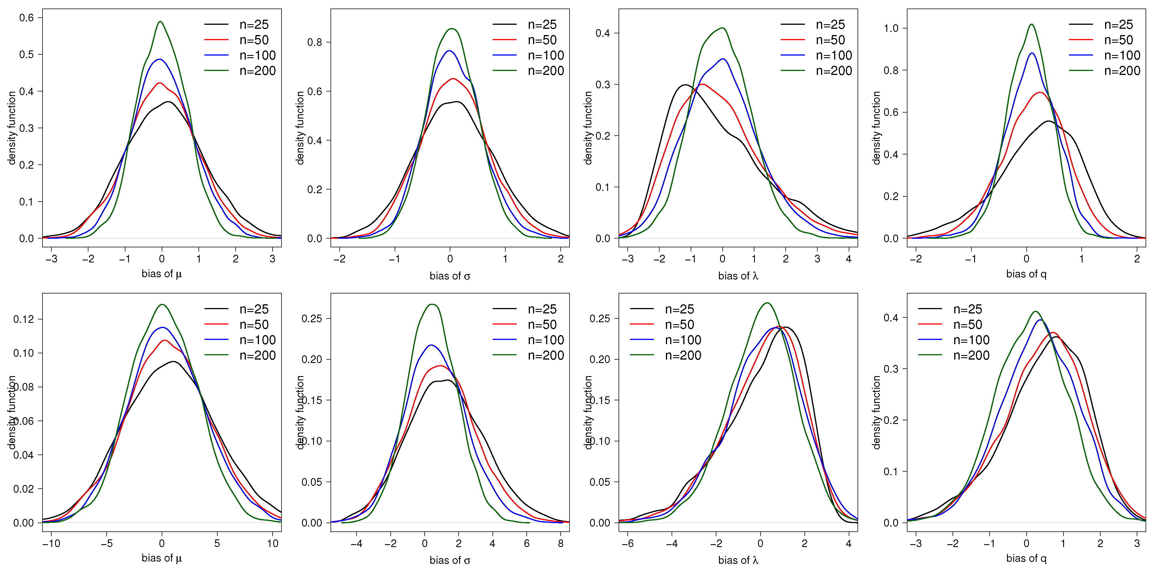
3. Simulation Study
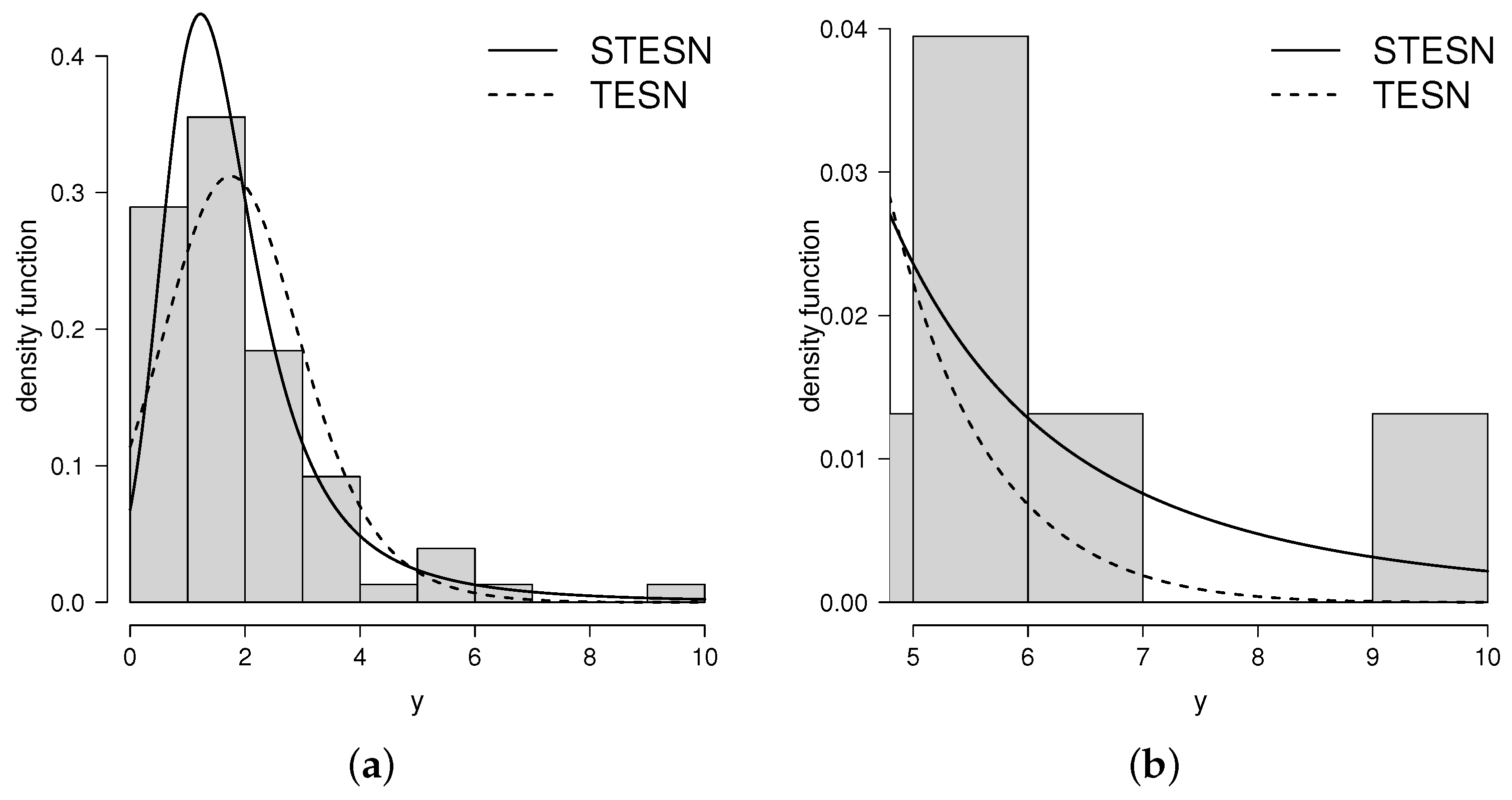
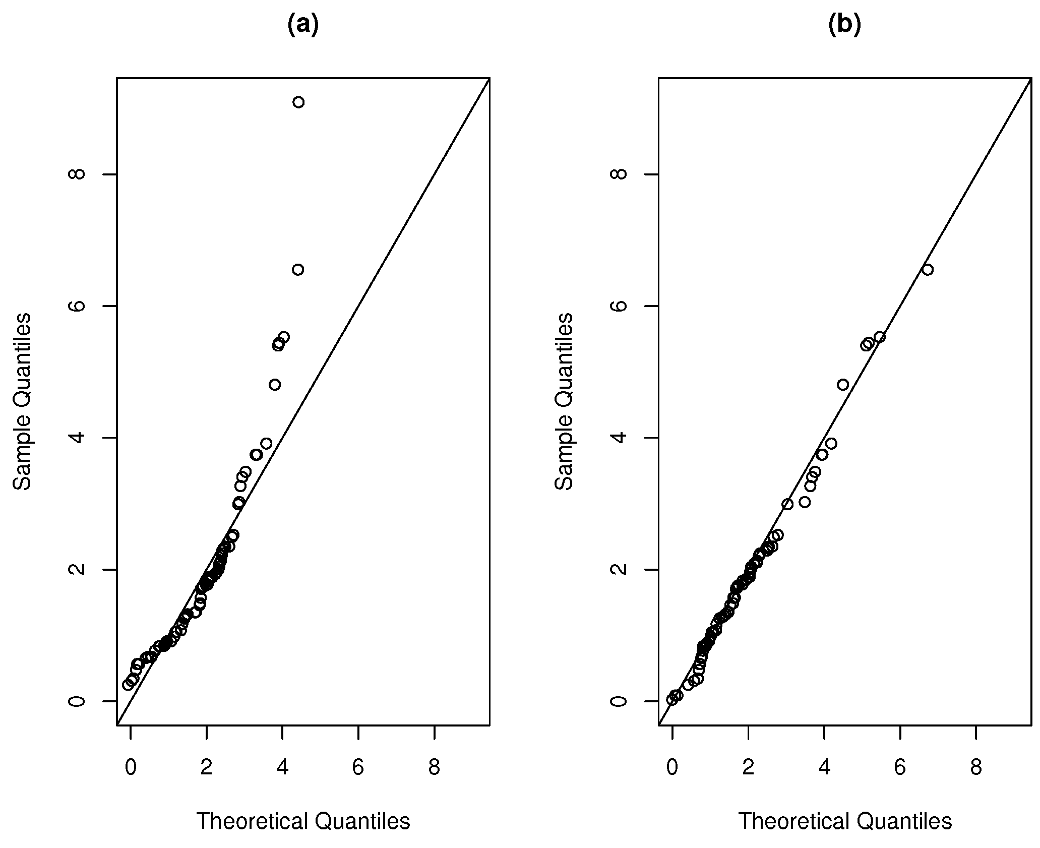
4. Application to a Data Set
5. Final Comments
Supplementary Materials
Author Contributions
Funding
Institutional Review Board Statement
Informed Consent Statement
Data Availability Statement
Conflicts of Interest
References
- Johnson, N.L.; Kotz, S.; Balakrishnan, N. Continuous Univariate Distributions, 2nd ed.; Wiley Series in Probability and Statistics; Wiley: New York, NY, USA, 1995. [Google Scholar]
- Rogers, W.H.; Tukey, J.W. Understanding some long-tailed symmetrical distributions. Stat. Neerl. 1972, 26, 211–226. [Google Scholar] [CrossRef]
- Mosteller, F.; Tukey, J.W. Data Analysis and Regression: A Second Course in Statistics; Addison-Wesley: Reading, MA, USA, 1977. [Google Scholar]
- Kadafar, K. A biweight approach to the one-sample problem. J. Am. Stat. Assoc. 1982, 77, 416–424. [Google Scholar] [CrossRef]
- Wang, J.; Boyer, J.; Genton, M.G. A skew-symmetric representation of multivariate distributions. Stat. Sin. 2004, 14, 1259–1270. [Google Scholar]
- Gómez, H.W.; Quintana, F.A.; Torres, F.J. New family of slash-distributions with elliptical contours. Stat. Probab. Lett. 2007, 77, 717–725. [Google Scholar] [CrossRef]
- Gómez, H.W.; Olivares-Pacheco, J.F.; Bolfarine, H. An extension of the generalized Birnbaum-Saunders distribution. Stat. Probab. Lett. 2009, 79, 331–338. [Google Scholar] [CrossRef]
- Nadarajah, S.; Nassiri, V.; Mohammadpour, A. Truncated-exponential skew-symmetric distributions. Statistics 2014, 48, 872–895. [Google Scholar] [CrossRef]
- Azzalini, A. A Class of Distributions Which Includes the Normal Ones. Scand. J. Stat. 1985, 12, 171–178. [Google Scholar]
- Ferreira, J.T.A.S.; Steel, M.F.J. A constructive representation of univariate skewed distributions. J. Am. Stat. Assoc. 2006, 101, 823–829. [Google Scholar] [CrossRef] [Green Version]
- Barreto-Souza, W.; Simas, A.B. The exp- G family of probability distributions. Braz. J. Probab. Stat. 2013, 27, 84–109. [Google Scholar] [CrossRef]
- Gomes, A.E.; Da-Silva, C.Q.; Cordeiro, G.M. The Exponentiated G Poisson Model. Commun. Stat.-Theory Methods 2015, 44, 4217–4240. [Google Scholar] [CrossRef]
- Maurya, S.K.; Nadarajah, S. Poisson Generated Family of Distributions: A Review. Sankhya B 2020, 1–57. [Google Scholar] [CrossRef]
- Lehmann, E.L. Elements of Large-Sample Theory; Springer: New York, NY, USA, 1999. [Google Scholar]
- R Development Core Team. A Language and Environment for Statistical Computing; R Foundation for Statistical Computing: Vienna, Austria, 2021. [Google Scholar]
- Borchers, H.W. Pracma: Practical Numerical Math Functions, R package version 2.3.3; 2021. Available online: https://CRAN.R-project.org/package=pracma (accessed on 24 June 2021).
- Akaike, H. A new look at the statistical model identification. IEEE Trans. Automat. Contr. 1974, 19, 716–723. [Google Scholar] [CrossRef]
- Schwarz, G. Estimating the dimension of a model. Ann. Stat. 1978, 6, 461–464. [Google Scholar] [CrossRef]
- Chernoff, H. On the distribution of the likelihood ratio. Ann. Stat. 1954, 54, 573–578. [Google Scholar] [CrossRef]
- Stram, D.O.; Lee, J.W. Variance components testing in the longitudinal mixed effects model. Biometrics 1994, 50, 1171–1177. [Google Scholar] [CrossRef] [PubMed]
- Gallardo, D.I.; Bolfarine, H.; Pedroso-de-Lima, A.C. A clustering cure rate model with application to a sealant study. J. Appl. Stat. 2017, 44, 2949–2962. [Google Scholar] [CrossRef]
- Maller, R.; Zhou, S. Testing for the Presence of Immune or Cured Individuals in Censored Survival Data. Biometrics 1995, 51, 1197–1205. [Google Scholar] [CrossRef] [PubMed]
- Barlow, R.E.; Toland, R.H.; Freeman, T. A Bayesian analysis of stress rupture life of Kevlar 49/epoxy spherical pressure vessels. In Procedings Conference on Applications of Statistics; Marcel Dekker: New York, NY, USA, 1984. [Google Scholar]


| True Values | ||||||||||||||||||||
|---|---|---|---|---|---|---|---|---|---|---|---|---|---|---|---|---|---|---|---|---|
| q | bias | SE | RMSE | CP | bias | SE | RMSE | CP | bias | SE | RMSE | CP | bias | SE | RMSE | CP | ||||
| 0 | 1 | −3 | 1 | 0.053 | 1.140 | 1.141 | 0.903 | 0.031 | 0.882 | 0.885 | 0.909 | 0.013 | 0.662 | 0.675 | 0.912 | 0.009 | 0.449 | 0.458 | 0.939 | |
| 0.084 | 0.489 | 0.496 | 0.972 | 0.069 | 0.367 | 0.373 | 0.965 | 0.052 | 0.278 | 0.287 | 0.961 | 0.042 | 0.197 | 0.203 | 0.959 | |||||
| −0.176 | 2.336 | 2.336 | 0.887 | −0.093 | 1.914 | 1.936 | 0.892 | −0.053 | 1.366 | 1.398 | 0.906 | −0.042 | 0.892 | 0.910 | 0.921 | |||||
| q | 0.195 | 0.587 | 0.618 | 0.973 | 0.119 | 0.350 | 0.370 | 0.972 | 0.082 | 0.220 | 0.235 | 0.965 | 0.057 | 0.151 | 0.161 | 0.961 | ||||
| 0 | 1 | −1 | 1 | −0.099 | 1.473 | 1.473 | 0.918 | −0.078 | 1.045 | 1.049 | 0.928 | −0.051 | 0.704 | 0.711 | 0.935 | −0.033 | 0.473 | 0.477 | 0.948 | |
| 0.159 | 0.532 | 0.555 | 0.970 | 0.111 | 0.372 | 0.388 | 0.965 | 0.075 | 0.252 | 0.263 | 0.958 | 0.044 | 0.179 | 0.184 | 0.953 | |||||
| −0.154 | 2.398 | 2.399 | 0.887 | −0.117 | 1.810 | 1.822 | 0.889 | −0.083 | 1.183 | 1.196 | 0.907 | −0.060 | 0.765 | 0.770 | 0.915 | |||||
| q | 0.214 | 0.555 | 0.594 | 0.962 | 0.163 | 0.479 | 0.506 | 0.960 | 0.080 | 0.229 | 0.243 | 0.958 | 0.041 | 0.147 | 0.152 | 0.953 | ||||
| 0 | 1 | 3 | 1 | −0.100 | 1.166 | 1.170 | 0.901 | −0.091 | 0.907 | 0.913 | 0.928 | −0.077 | 0.615 | 0.624 | 0.936 | −0.047 | 0.448 | 0.458 | 0.945 | |
| 0.094 | 0.512 | 0.514 | 0.974 | 0.076 | 0.394 | 0.401 | 0.968 | 0.056 | 0.254 | 0.261 | 0.961 | 0.053 | 0.194 | 0.201 | 0.957 | |||||
| 0.251 | 2.300 | 2.299 | 0.871 | 0.192 | 1.843 | 1.875 | 0.896 | 0.167 | 1.295 | 1.322 | 0.917 | 0.094 | 0.864 | 0.887 | 0.925 | |||||
| q | 0.168 | 0.657 | 0.678 | 0.965 | 0.115 | 0.376 | 0.393 | 0.961 | 0.071 | 0.220 | 0.231 | 0.960 | 0.045 | 0.148 | 0.154 | 0.959 | ||||
| 0 | 1 | −2 | 2 | −0.061 | 1.140 | 1.139 | 0.905 | −0.033 | 1.097 | 1.097 | 0.918 | −0.031 | 0.941 | 0.950 | 0.929 | −0.010 | 0.664 | 0.672 | 0.932 | |
| 0.053 | 0.386 | 0.389 | 0.986 | 0.042 | 0.343 | 0.357 | 0.979 | 0.034 | 0.297 | 0.318 | 0.971 | 0.025 | 0.189 | 0.200 | 0.964 | |||||
| −0.192 | 2.875 | 2.880 | 0.894 | −0.151 | 2.778 | 2.783 | 0.901 | −0.122 | 2.318 | 2.355 | 0.915 | −0.097 | 1.625 | 1.652 | 0.921 | |||||
| q | 0.362 | 1.301 | 1.350 | 0.971 | 0.278 | 1.254 | 1.341 | 0.969 | 0.226 | 1.008 | 1.094 | 0.963 | 0.180 | 0.510 | 0.541 | 0.959 | ||||
| 0 | 1 | 3 | 2 | −0.205 | 1.004 | 1.024 | 0.899 | −0.079 | 0.915 | 0.918 | 0.910 | −0.061 | 0.758 | 0.762 | 0.928 | −0.044 | 0.580 | 0.581 | 0.936 | |
| 0.079 | 0.389 | 0.389 | 0.971 | 0.053 | 0.313 | 0.314 | 0.968 | 0.041 | 0.264 | 0.271 | 0.961 | 0.030 | 0.201 | 0.205 | 0.959 | |||||
| 0.278 | 2.655 | 2.668 | 0.896 | 0.212 | 2.570 | 2.569 | 0.906 | 0.144 | 2.100 | 2.127 | 0.917 | 0.100 | 1.566 | 1.578 | 0.929 | |||||
| q | 0.213 | 1.256 | 1.273 | 0.965 | 0.192 | 1.035 | 1.075 | 0.961 | 0.119 | 0.880 | 0.926 | 0.959 | 0.099 | 0.507 | 0.529 | 0.958 | ||||
| 0 | 1 | 2 | 2 | 0.164 | 1.171 | 1.191 | 0.904 | 0.115 | 1.114 | 1.115 | 0.912 | 0.079 | 0.901 | 0.904 | 0.939 | 0.052 | 0.689 | 0.693 | 0.945 | |
| 0.099 | 0.369 | 0.369 | 0.986 | 0.082 | 0.335 | 0.350 | 0.982 | 0.074 | 0.280 | 0.299 | 0.971 | 0.040 | 0.204 | 0.215 | 0.960 | |||||
| 0.381 | 3.081 | 3.103 | 0.866 | 0.242 | 2.772 | 2.782 | 0.899 | 0.171 | 2.252 | 2.267 | 0.919 | 0.127 | 1.668 | 1.683 | 0.935 | |||||
| q | 0.280 | 1.318 | 1.347 | 0.976 | 0.223 | 1.137 | 1.213 | 0.973 | 0.112 | 1.023 | 1.103 | 0.967 | 0.087 | 0.583 | 0.629 | 0.959 | ||||
| 0 | 1 | −1 | 3 | 0.023 | 1.102 | 1.102 | 0.919 | 0.022 | 1.059 | 1.059 | 0.932 | 0.005 | 1.013 | 1.013 | 0.938 | 0.004 | 0.913 | 0.914 | 0.941 | |
| 0.102 | 0.321 | 0.321 | 0.979 | 0.071 | 0.246 | 0.256 | 0.975 | 0.068 | 0.222 | 0.251 | 0.971 | 0.057 | 0.191 | 0.224 | 0.961 | |||||
| −0.134 | 3.189 | 3.188 | 0.972 | −0.116 | 3.001 | 3.002 | 0.965 | −0.072 | 2.726 | 2.725 | 0.961 | −0.049 | 2.414 | 2.417 | 0.955 | |||||
| q | 0.386 | 1.835 | 1.837 | 0.974 | 0.320 | 1.526 | 1.582 | 0.970 | 0.202 | 1.420 | 1.484 | 0.965 | 0.170 | 1.258 | 1.244 | 0.961 | ||||
| 0 | 1 | 2 | 3 | 0.128 | 1.014 | 1.022 | 0.899 | 0.069 | 0.930 | 0.930 | 0.912 | 0.061 | 0.830 | 0.832 | 0.943 | 0.046 | 0.813 | 0.815 | 0.944 | |
| 0.134 | 0.324 | 0.325 | 0.984 | 0.079 | 0.274 | 0.278 | 0.977 | 0.052 | 0.246 | 0.266 | 0.962 | 0.049 | 0.209 | 0.227 | 0.959 | |||||
| 0.159 | 2.939 | 2.942 | 0.888 | 0.128 | 2.739 | 2.752 | 0.911 | 0.116 | 2.643 | 2.655 | 0.927 | 0.082 | 2.253 | 2.264 | 0.935 | |||||
| q | 0.322 | 1.556 | 1.556 | 0.981 | 0.262 | 1.411 | 1.475 | 0.972 | 0.174 | 1.271 | 1.237 | 0.961 | 0.054 | 1.027 | 1.039 | 0.958 | ||||
| −5 | 4 | −2 | 2 | −0.354 | 4.484 | 4.495 | 0.900 | −0.225 | 4.405 | 4.405 | 0.917 | −0.137 | 3.562 | 3.600 | 0.927 | −0.040 | 2.641 | 2.670 | 0.935 | |
| 0.317 | 1.550 | 1.553 | 0.970 | 0.281 | 1.311 | 1.365 | 0.964 | 0.237 | 1.070 | 1.132 | 0.958 | 0.170 | 0.793 | 0.837 | 0.957 | |||||
| −0.247 | 2.862 | 2.861 | 0.885 | −0.223 | 2.808 | 2.817 | 0.906 | −0.191 | 2.240 | 2.273 | 0.919 | −0.130 | 1.631 | 1.658 | 0.929 | |||||
| q | 0.309 | 1.292 | 1.328 | 0.974 | 0.245 | 1.155 | 1.237 | 0.966 | 0.222 | 0.851 | 0.909 | 0.961 | 0.157 | 0.581 | 0.617 | 0.955 | ||||
| 10 | 16 | 1 | 3 | 0.677 | 17.507 | 17.571 | 0.912 | 0.594 | 13.643 | 13.944 | 0.914 | 0.430 | 11.891 | 11.889 | 0.926 | 0.184 | 9.222 | 9.240 | 0.945 | |
| 1.237 | 4.948 | 4.951 | 0.904 | 0.957 | 4.159 | 4.205 | 0.927 | 0.651 | 3.454 | 3.827 | 0.937 | 0.480 | 2.030 | 2.113 | 0.949 | |||||
| 0.128 | 3.206 | 3.204 | 0.898 | 0.118 | 3.084 | 3.088 | 0.915 | 0.102 | 2.726 | 2.727 | 0.922 | 0.075 | 2.339 | 2.344 | 0.938 | |||||
| q | 0.470 | 1.401 | 1.401 | 0.981 | 0.453 | 1.273 | 1.240 | 0.979 | 0.333 | 1.087 | 1.052 | 0.961 | 0.142 | 0.927 | 0.938 | 0.959 | ||||
| n | S | |||||
|---|---|---|---|---|---|---|
| 76 |
| Estimations | TESN | STESN |
|---|---|---|
| q | – | |
| log-likelihood | ||
| AIC | ||
| BIC | ||
| KSS | ||
| p-value |
Publisher’s Note: MDPI stays neutral with regard to jurisdictional claims in published maps and institutional affiliations. |
© 2021 by the authors. Licensee MDPI, Basel, Switzerland. This article is an open access article distributed under the terms and conditions of the Creative Commons Attribution (CC BY) license (https://creativecommons.org/licenses/by/4.0/).
Share and Cite
Rivera, P.A.; Gallardo, D.I.; Venegas, O.; Bourguignon, M.; Gómez, H.W. An Extension of the Truncated-Exponential Skew- Normal Distribution. Mathematics 2021, 9, 1894. https://doi.org/10.3390/math9161894
Rivera PA, Gallardo DI, Venegas O, Bourguignon M, Gómez HW. An Extension of the Truncated-Exponential Skew- Normal Distribution. Mathematics. 2021; 9(16):1894. https://doi.org/10.3390/math9161894
Chicago/Turabian StyleRivera, Pilar A., Diego I. Gallardo, Osvaldo Venegas, Marcelo Bourguignon, and Héctor W. Gómez. 2021. "An Extension of the Truncated-Exponential Skew- Normal Distribution" Mathematics 9, no. 16: 1894. https://doi.org/10.3390/math9161894
APA StyleRivera, P. A., Gallardo, D. I., Venegas, O., Bourguignon, M., & Gómez, H. W. (2021). An Extension of the Truncated-Exponential Skew- Normal Distribution. Mathematics, 9(16), 1894. https://doi.org/10.3390/math9161894