High-Dimensional Mahalanobis Distances of Complex Random Vectors

Abstract

In this paper, we investigate the asymptotic distributions of two types of Mahalanobis distance (MD): leave-one-out MD and classical MD with both Gaussian- and non-Gaussian-distributed complex random vectors, when the sample size n and the dimension of variables p increase under a fixed ratio $c=p/n\to \infty$. We investigate the distributional properties of complex MD when the random samples are independent, but not necessarily identically distributed. Some results regarding the F-matrix $\mathit{F}={\mathit{S}}_2^{-1}{\mathit{S}}_1$—the product of a sample covariance matrix ${\mathit{S}}_1$ (from the independent variable array $(\mathit{b}e{\left(Z_i\right)}_{1\times n}$) with the inverse of another covariance matrix ${\mathit{S}}_2$ (from the independent variable array ${\left({\mathit{Z}}_{j\ne i}\right)}_{p\times n}$)—are used to develop the asymptotic distributions of MDs. We generalize the F-matrix results so that the independence between the two components ${\mathit{S}}_1$ and ${\mathit{S}}_2$ of the F-matrix is not required.

1. Introduction

Mahalanobis distance (MD) is a fundamental statistic in multivariate analysis. It is used to measure the distance between two random vectors or the distance between a random vector and its center of distribution. MD has received wide attention since it was proposed by Mahalanobis [1] in the 1930’s. After decades of development, MD has been applied as a distance metric in various research areas, including propensity score analysis, as well as applications in matching [2], classification and discriminant analysis [3]. In the former case, MD is used to calculate the propensity scores as a measurement of the difference between two objects. In the latter case, the differences among the clusters are investigated based on MD. The applications of MD are also related to multivariate calibration [4], psychological analysis [5] and the construction of multivariate process control charts [6]; it is a standard method to assess the similarity between the observations.

As an essential scale for distinguishing objects from each other, the robustness of MD is important for guaranteeing the accuracy of an analysis. Thus, the properties of MD have been investigated in the last decade. Gath and Hayes [7] investigated the bounds for extreme MDs. Dai et al. [8] derived a number of marginal moments of the sample MD and showed that it behaves unexpectedly when p is relatively larger than n. Dai and Holgersson [9] examined the marginal behavior of MDs and determined their density functions. With the distribution derived by Dai and Holgersson [9], one can set the inferential boundaries for the MD itself and acquire robust criteria. Beside the developments above, some attention has been paid to the Fisher matrix (F-matrix) and Beta matrix which can be considered as the generalizations of MD.

We provide the definition of the Fisher matrix (see [10]) which is essential here. The Fisher matrices, or simply F -matrices, are an ensemble of matrices with two components each. Let $\left\{Z_{jk},j,k=1,2,\dots \right\}$ be either both real or both complex random variable arrays. For $p\ge 1$ and $n\ge 1$, let

$$\begin{array}{c}\mathit{Z}=\left(Z_{jk}:1\le j\le p,1\le k\le n\right)=\left({\mathit{Z}}_{·1},\dots ,{\mathit{Z}}_{·n}\right),\hfill \\ {\mathit{z}}_{\left(i\right)}=\left(z_i:1\le i\le n,i\ne k\right)={\mathit{Z}}_{·i},\hfill \end{array}$$

be the arrays, with column vectors $\left({\mathit{Z}}_{·k}\right)$. The ${\mathit{z}}_{\left(i\right)}$ corresponds to the ith observation in $\mathit{Z}$. This observation is isolated from the rest of the observations, so that ${\mathit{z}}_{\left(i\right),i\ne k,(p\times 1)}$ and ${\mathit{Z}}_{p\times (n-1)}$ are two independent samples. We determine the following matrices:

$$\begin{array}{c}{\mathit{S}}_1={\mathit{z}}_{\left(i\right),i\ne k}{\mathit{z}}_{\left(i\right),i\ne k}^{*}={\mathit{z}}_{\left(i\right)}{\mathit{z}}_{\left(i\right)}^{*},\hfill \\ {\mathit{S}}_2=\frac{1}{n}\sum _{k=1}^n{\mathit{Z}}_{·k}{\mathit{Z}}_{·k}^{*}=\frac{1}{n}\mathit{Z}{\mathit{Z}}^{*},\hfill \end{array}$$

where ${}^{*}$ stands for complex conjugate transpose. These two matrices are both of size $p\times p.$ Then the Fisher matrix (or F -matrix) is defined as

$$\mathit{F}:={\mathit{S}}_1{\mathit{S}}_2^{-1}.$$

Pillai [11], Pillai and Flury [12] and Bai et al. [13] have studied the spectral properties of the F-distribution. Johansson [14] investigated the central limit theorem (CLT) for the random Hermitian matrices, including the Gaussian unitary ensemble. Guionnet [15] established the CLT for the non-commutative functional of Gaussian large random matrices. Bai et al. [16] obtain the CLT for the linear spectral statistics of the Wigner matrix. Zheng [10] extends the moments of the F-matrix into non-Gaussian circumstances with the assumption that the two components ${\mathit{S}}_1$ and ${\mathit{S}}_2$ of an F-matrix $\mathit{F}={\mathit{S}}_2^{-1}{\mathit{S}}_1$ are independent. Gallego et al. [17] extended the MD into the condition of a multidimensional Normal distribution and studied the properties of MD for this case.

However, to the best of our knowledge, the properties of MDs with non-Gaussian complex random variables have not been studied much in the literature. In this paper, we derive the CLT for an MD with complex random variables under a more general circumstance. The common restrictions on the random vector, such as independent and identically distributed (i.i.d.) for the random sample, are not required. The independence between the two components ${\mathit{S}}_1$ and ${\mathit{S}}_2$ of the F-matrix $\mathit{F}={\mathit{S}}_2^{-1}{\mathit{S}}_1$ is relaxed. We investigate the distributional properties of complex MD without assuming normal distribution. The fourth moments of the MDs are allowed to be an arbitrary value.

This paper is organized as follows. In Section 2, we introduce the basic definitions concerning different types of complex random vectors, their covariance matrix, and the corresponding MDs. In Section 3, the first moments of different types of MDs and their distribution properties are given. The connection of leave-one-out MD and classical MD is derived, and their respective asymptotic distributions under general assumptions are investigated. We end up this paper by giving some concluding remarks and discussions in Section 4.

Some Examples of Mahalanobis Distance in Signal Processing

MD has been applied in different research areas. We give two examples that are related to the applications of MD in signal processing.

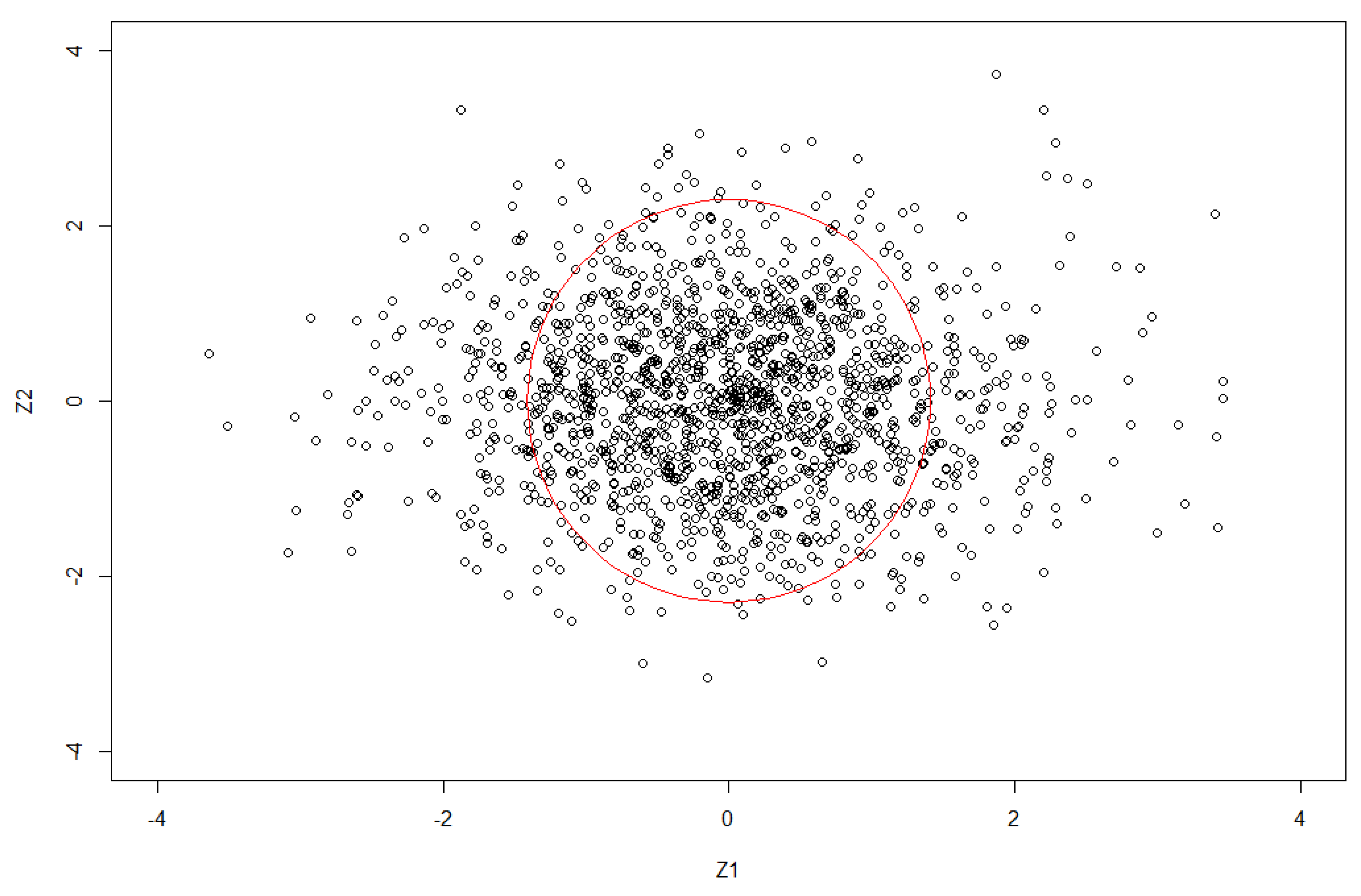
Example 1.

We illustrate our idea by using an example. In Figure 1, each point corresponds to the real and comlex part of an MD. The circle in red is an inferential boundary with the radius calculated based on MDs. The points that are outside the boundary are considered to be signals, while the points that are lying inside the circle are detected as noise.

This example has been used in some research; for example, in evaluating the capacity of multiple-input, multiple-output (MIMO) wireless communication systems (see [18] for more details). Denote the number of inputs (or transmitters) and the number of outputs (or receivers) of the MIMO wireless communication system by $n_t$ and $n_r$ respectively, and assume that the channel coefficients are correlated at both the transmitter and the receiver ends. Then the MIMO channel can be represented by an $n_r\times n_t$ complex random matrix $\mathit{H}$ with corresponding covariance matrices ${\mathsf{\Sigma }}_r$ and ${\mathsf{\Sigma }}_t$. For most of the cases, ${\mathsf{\Sigma }}_r$ and ${\mathsf{\Sigma }}_t$ should be replaced by the sample covariance matrices ${\mathit{S}}_r$ and ${\mathit{S}}_t$ to represent the channel correlations at the receiver and transmitter ends, respectively. The information processed by this random channel is a random quantity which can be measured by MD.

Example 2.

Zhao et al. [19] use MD in a fuzzy clustering algorithm in order to reduce the effect of noise on image segmentation. They compare the boundaries of clusters calculated by both the Euclidean distance and MD. The boundaries calculated by the Euclidean distance are straight lines which misclassify the observations that diverge far from their cluster center, while the boundaries based on the MDs are curves that fit better with the covariance of the cluster. This example implies that the MD is more accurate with regards to the measure of dissimilarity for image segmentation. It can be extended to the application of clustering when the channel signals are complex random variables.

2. Preliminaries

In this section, some important definitions of complex random variables and related concepts are introduced, including the covariance matrix of a complex random vector and the corresponding MDs.

We first define the covariance matrix of a general complex random vector on an $n\times p$ dimension complex random variable $\mathit{z}$ where p is the number of variables and n is the sample size of the dataset, as given in [20]:

Definition 1.

Let ${\mathit{z}}_j=(z_1,\dots ,z_p)\in {\mathbb{C}}^p$, $j=1,\dots ,n$ be a complex random vector with known mean $E\left[{\mathit{z}}_j\right]={\mu }_{z,j}$ where ${\mathit{z}}_j={\mathit{x}}_j+i{\mathit{y}}_j$, $i=\sqrt{-1}$ and ${\mathit{x}}_j,{\mathit{y}}_j\in {\mathbb{R}}^p$. Let ${\mathsf{\Gamma }}_{p\times p}$ be the covariance matrix and ${\mathit{C}}_{p\times p}$ be the relation matrix of ${\mathit{z}}_j$ respectively. Then ${\mathsf{\Gamma }}_{p\times p}$ and ${\mathit{C}}_{p\times p}$ are defined respectively as follows:

$$\mathsf{\Gamma }=E\left[({\mathit{z}}_j-{\mathit{\mu }}_{z,j}){({\mathit{z}}_j-{\mathit{\mu }}_{z,j})}^{*}\right],$$

$$\mathit{C}=E\left[\left({\mathit{z}}_j-{\mathit{\mu }}_{z,j}\right){\left({\mathit{z}}_j-{\mathit{\mu }}_{z,j}\right)}^{\prime }\right],$$

where ${}^{\prime }$ is the transpose.

Definition 1 shows a general presentation of the complex random variables without imposing any distributional assumption on ${\mathit{z}}_j$. If we set the components of ${\mathit{z}}_j$, the random variables ${\mathit{x}}_j$ and ${\mathit{y}}_j$, as normally distributed, then we are in a more familiar context in the complex space: circular symmetricity. The circular symmetricity of a complex normal random variable is an assumption that is used for the standardized form of complex Gaussian-distributed random variables. The definition of circular symmetricity is the following.

Definition 2.

A p-dimensional complex random variable ${\mathit{z}}_{p\times 1}={\mathit{x}}_{p\times 1}+i{\mathit{y}}_{p\times 1}$ is a circularly symmetric complex normal one if the vector $vec{\left[\mathit{x}\mathit{y}\right]}^{\prime }$ is normally distributed, i.e.,

$${\displaystyle \left(\begin{array}{c}{\mathit{x}}_{p\times 1}\\ {\mathit{y}}_{p\times 1}\end{array}\right)\sim N\left(\left[\begin{array}{c}Re{\mathit{\mu }}_{z,p\times 1}\\ Im{\mathit{\mu }}_{z,p\times 1}\end{array}\right],\frac{1}{2}\left[\begin{array}{cc}Re{\mathsf{\Gamma }}_{z,p\times 1}& -Im{\mathsf{\Gamma }}_{z,p\times 1}\\ Im{\mathsf{\Gamma }}_{z,p\times 1}& Re{\mathsf{\Gamma }}_{z,p\times 1}\end{array}\right]\right),}$$

where ${\mathit{\mu }}_{z,p\times 1}=E\left[\mathit{z}\right]$ and ${\mathsf{\Gamma }}_{z,p\times p}=E\left[(\mathit{z}-{\mathit{\mu }}_z){(\mathit{z}-{\mathit{\mu }}_z)}^{*}\right]$, “$Re$” stands for the real part and “$Im$” stands for the imaginary part.

The circularly symmetric normally distributed complex random variable can be used in the circumstance of a standard normal distribution in real space to simplify the derivations on complex random variables. Based on this condition, we acquire a simplified probability density function (hereinafter p.d.f.) on a complex normal random vector which is presented in the following example.

Example 3.

The circularly symmetric complex random vector $\mathit{z}={(z_1,\dots ,z_p)}^{\prime }\in {\mathbb{C}}^p$ with mean vector ${\mathit{\mu }}_z=\mathit{0}$ and relation matrix $\mathit{C}=\mathit{0}$ has the p.d.f. as follows:

$$f\left(\mathit{z}\right)=\frac{1}{{\pi }^p\left|\mathit{z}\right|}exp(-{\mathit{z}}^{*}{\mathsf{\Gamma }}_z^{-1}\mathit{z}),$$

where ${\mathsf{\Gamma }}_z$ is the covariance matrix of $\mathit{z}$ and “$|.|$” is the determinant.

Based on Example 3, one can see the possibility of transforming the expression of a complex random vector into a form consisting of vector multiplication between a complex constant vector and a real random vector. Let $z_j$ be a complex random variable; then, the transformation between a complex random variable and its real random variables can be presented as follows:

$$z_j=\mathit{J}\left(\begin{array}{c}{x}_j\\ y_j\end{array}\right),where\mathit{J}=\left(\begin{array}{cc}1& i\end{array}\right).$$

The transformation offers a different way of inspecting the complex random vector [21]. The complex random vector can be considered as the bivariate form of a real random vector pre-multiplied by a constant vector. This transformation offers another way to present the complex covariance matrix in the form of real random vectors. The idea is presented by the example as follows.

Define matrices ${\mathsf{\Gamma }}_{xx}=E\left[\left(\mathit{x}-Re\mathit{\mu }\right){\left(\mathit{x}-Re\mathit{\mu }\right)}^{\prime }\right]$, ${\mathsf{\Gamma }}_{yy}=E\left[\left(\mathit{y}-Im\mathit{\mu }\right){\left(\mathit{y}-Im\mathit{\mu }\right)}^{\prime }\right]$, ${\mathsf{\Gamma }}_{xy}=E\left[\left(\mathit{x}-Re\mathit{\mu }\right){\left(\mathit{y}-Im\mathit{\mu }\right)}^{\prime }\right]$ and ${\mathsf{\Gamma }}_{yx}=E\left[\left(\mathit{y}-Im\mathit{\mu }\right){\left(\mathit{x}-Re\mathit{\mu }\right)}^{\prime }\right]$. The covariance matrix $\mathsf{\Gamma }$ of a p-dimensional complex random vector can be represented in the form of real random vectors $\mathit{x}$ and $\mathit{y}$, as follows:

$${\mathsf{\Gamma }}_{z,2p\times 2p}=\left(\begin{array}{cc}{\mathsf{\Gamma }}_{xx}& {\mathsf{\Gamma }}_{xy}\\ {\mathsf{\Gamma }}_{yx}& {\mathsf{\Gamma }}_{yy}\end{array}\right).$$

3. MD on Complex Random Variables

In this section, we introduce two types of MDs given in Definitions 5 and 6. We start with the classical MD which is based on a known mean and a known covariance matrix. The definition is given as follows.

Definition 3.

The MD of the complex random vector ${\mathit{z}}_j\in {\mathbb{C}}^p,j=1,\dots ,n$ with known mean μ and known covariance matrix ${\mathsf{\Gamma }}_z$ is defined as follows:

$$\begin{array}{ccc}\hfill D\left({\mathsf{\Gamma }}_z,{\mathit{z}}_j,\mathit{\mu }\right)& =& {\left({\mathit{z}}_j-\mathit{\mu }\right)}^{*}{\mathsf{\Gamma }}_z^{-1}\left({\mathit{z}}_j-\mathit{\mu }\right).\hfill \end{array}$$

(1)

There are both real and complex parts for a complex random vector. Thus, we define the corresponding MDs of the two components in a complex random variable.

Definition 4.

The MDs on the real part and imaginary part ${\mathit{x}}_j,{\mathit{y}}_j\in {\mathbb{R}}^p,j=1,\dots ,n$ of a complex random vector ${\mathit{z}}_j\in {\mathbb{C}}^p,j=1,\dots ,n$ with known mean μ and known covariance matrix ${\mathsf{\Gamma }}_{..}$ are defined as follows:

$$\begin{array}{ccc}& & D\left({\mathsf{\Gamma }}_{xx},{\mathit{x}}_j,Re\mathit{\mu }\right)={\left({\mathit{x}}_j-Re\mathit{\mu }\right)}^{*}{\mathsf{\Gamma }}_{xx}^{-1}\left({\mathit{x}}_j-Re\mathit{\mu }\right),\hfill \end{array}$$

(2)

$$\begin{array}{ccc}& & D\left({\mathsf{\Gamma }}_{yy},{\mathit{y}}_j,Im\mathit{\mu }\right)={\left({\mathit{y}}_j-Im\mathit{\mu }\right)}^{*}{\mathsf{\Gamma }}_{yy}^{-1}\left({\mathit{y}}_j-Im\mathit{\mu }\right).\hfill \end{array}$$

(3)

Under the definitions above, we can derive the distribution of the MDs on a complex random vector with known mean and covariance. We present the distribution as follows.

Proposition 1.

Let $\mathit{Z}$ be an $n\times p$ row-wise double array of i.i.d. complex normally distributed random variables with $E\left[{\mathit{z}}_{.j}\right]=\mathit{0}$, $j=1,\dots ,p$ and complex positive definite Hermitian covariance matrix ${\mathsf{\Gamma }}_z$. Then we have the distribution of the MD in (1) as $D\left({\mathsf{\Gamma }}_z,{\mathit{z}}_i,\mathit{0}\right)\sim {\chi }_{2p}^2$.

Proof. 

For the proof of this proposition, the reader can refer to reference [22]. □

The result of Proposition 1 is employed here to derive the moments of the MDs on the real and complex parts below.

Proposition 2.

The first moment of $D\left({\mathsf{\Gamma }}_z,{\mathit{z}}_j,\mathit{0}\right)$ defined in (1) is given as follows:

$$E\left[D\left({\mathsf{\Gamma }}_z,{\mathit{z}}_j,\mathit{0}\right)\right]=2p.$$

Proof. 

The result follows Proposition 1. □

Theorem 1.

Set the random variables ${\mathit{x}}_i$ and ${\mathit{y}}_i$ to be normally distributed, and the covariance of $D\left({\mathsf{\Gamma }}_{xx},{\mathit{x}}_i,\mathit{0}\right)$ and $D\left({\mathsf{\Gamma }}_{yy},{\mathit{y}}_i,\mathit{0}\right)$ as given in (2) and (3). Then their distributions are given as follows:

$$Cov\left[D\left({\mathsf{\Gamma }}_{xx},{\mathit{x}}_i,\mathit{0}\right),D\left({\mathsf{\Gamma }}_{yy},{\mathit{y}}_i,\mathit{0}\right)\right]=tr\left[{\mathsf{\Gamma }}_{xx}^{-1}\otimes {\mathsf{\Gamma }}_{yy}^{-1}\Phi \right]-p^2,$$

$$\left(\begin{array}{c}D\left({\mathsf{\Gamma }}_{xx},{\mathit{x}}_j,\mathit{0}\right)\\ D\left({\mathsf{\Gamma }}_{yy},{\mathit{y}}_j,\mathit{0}\right)\end{array}\right)\sim \left(\begin{array}{c}{\chi }_p^2\\ {\chi }_p^2\end{array}\right),$$

where ⊗ is the tensor product, $\mathsf{\Phi }=E\left({\mathit{x}}_j{{\mathit{x}}_j}^{\prime }\otimes {\mathit{y}}_j{{\mathit{y}}_j}^{\prime }\right)$ and $tr(.)$ stands for trace.

Proof. 

Proposition 1 shows $D\left({\mathsf{\Gamma }}_{yy},{\mathit{y}}_j,\mathit{0}\right)\sim {\chi }_p^2$ and $D\left({\mathsf{\Gamma }}_{xx},{\mathit{x}}_j,\mathit{0}\right)\sim {\chi }_p^2.$ In order to derive the covariance of these two MDs, we need to first derive their cross moments.

$$\begin{array}{ccc}& & E\left({\mathit{x}}^{\prime }{\mathsf{\Gamma }}_{xx}^{-1}\mathit{x}{\mathit{y}}^{\prime }{\mathsf{\Gamma }}_{yy}^{-1}\mathit{y}\right)=Etr\left[\left({\mathit{x}}^{\prime }\otimes {\mathit{y}}^{\prime }\right)\left({\mathsf{\Gamma }}_{xx}^{-1}\otimes {\mathsf{\Gamma }}_{yy}^{-1}\right)\left(\mathit{x}\otimes \mathit{y}\right)\right]\hfill \\ \hfill =& & Etr\left[\left({\mathsf{\Gamma }}_{xx}^{-1}\otimes {\mathsf{\Gamma }}_{yy}^{-1}\right)\left(\mathit{x}\otimes \mathit{y}\right)\left({\mathit{x}}^{\prime }\otimes {\mathit{y}}^{\prime }\right)\right]=Etr\left[\left({\mathsf{\Gamma }}_{xx}^{-1}\otimes {\mathsf{\Gamma }}_{yy}^{-1}\right)\left(\mathit{x}{\mathit{x}}^{\prime }\otimes \mathit{y}{\mathit{y}}^{\prime }\right)\right]\hfill \\ \hfill =& & tr\left[\left({\mathsf{\Gamma }}_{xx}^{-1}\otimes {\mathsf{\Gamma }}_{yy}^{-1}\right)E\left(\mathit{x}{\mathit{x}}^{\prime }\otimes \mathit{y}{\mathit{y}}^{\prime }\right)\right].\hfill \end{array}$$

Thus, the covariance is given as follows:

$$\begin{array}{ccc}& & Cov\left[D\left({\mathsf{\Gamma }}_{xx},{\mathit{x}}_j,\mathit{0}\right),D\left({\mathsf{\Gamma }}_{yy},{\mathit{y}}_j,\mathit{0}\right)\right]\hfill \\ & & =E\left[D\left({\mathsf{\Gamma }}_{xx},{\mathit{x}}_j,\mathit{0}\right)D\left({\mathsf{\Gamma }}_{yy},{\mathit{y}}_j,\mathit{0}\right)\right]-E\left[D\left({\mathsf{\Gamma }}_{xx},{\mathit{x}}_j,\mathit{0}\right)\right]E\left[D\left({\mathsf{\Gamma }}_{yy},{\mathit{y}}_j,\mathit{0}\right)\right]\hfill \\ & & =E\left[D\left({\mathsf{\Gamma }}_{xx},{\mathit{x}}_j,\mathit{0}\right)D\left({\mathsf{\Gamma }}_{yy},{\mathit{y}}_j,\mathit{0}\right)\right]-p^2\hfill \\ & & =tr\left[\left({\mathsf{\Gamma }}_{xx}^{-1}\otimes {\mathsf{\Gamma }}_{yy}^{-1}\right)\mathsf{\Phi }\right]-p^2,\hfill \end{array}$$

which completes the proof. □

The results presented so far concern a complex random vector with known mean and known covariance matrix. In practice, the mean $\mathit{\mu }$ and covariance matrix ${\mathsf{\Gamma }}_z$ are not available all the time. Thus, some alternative statistics such as sample mean $\overline{\mathit{z}}=n^{-1}{\sum }_{j=1}^n{\mathit{z}}_j$ and sample covariance ${\mathit{S}}_z=n^{-1}{\sum }_{j=1}^n\left({\mathit{z}}_j-\overline{\mathit{z}}\right){\left({\mathit{z}}_j-\overline{\mathit{z}}\right)}^{*}$ are used as substitutions of the population mean and variance when building the MDs.

We introduce the definitions of MDs with sample mean and sample covariance matrix in the following.

Definition 5.

Let ${\mathit{z}}_j\in {\mathbb{C}}^p,j=1,\dots ,n$, be a complex normally distributed random sample. The MD on the complex random vector ${\mathit{z}}_j$ with sample mean $\overline{\mathit{z}}=n^{-1}{\sum }_{j=1}^n{z}_j$ and sample covariance matrix ${\mathit{S}}_z={(n-1)}^{-1}{\sum }_{j=1}^n\left({\mathit{z}}_j-\overline{\mathit{z}}\right){\left({\mathit{z}}_j-\overline{\mathit{z}}\right)}^{*}$ is defined as follows:

$$\begin{array}{c}\hfill D_j=D\left({\mathit{S}}_z,{\mathit{z}}_j,\overline{\mathit{z}}\right)={\left({\mathit{z}}_j-\overline{\mathit{z}}\right)}^{*}{\mathit{S}}_z^{-1}\left({\mathit{z}}_j-\overline{\mathit{z}}\right).\end{array}$$

(4)

For the purpose of deriving further distributional properties, we give an alternative definition of an MD: the leave-one-out case. Leave-one-out here means that we remove one observation each time and use the rest of the observations for constructing the MD.

Definition 6.

Let the leave-one-out sample mean of a complex random vector be ${\overline{\mathit{z}}}_{\left(i\right)}={\left(n-1\right)}^{-1}$${\sum }_{j=1,j\ne i}^n{\mathit{z}}_j$ and the corresponding leave-one-out sample covariance matrix ${\mathit{S}}_{\left(i\right)}={\left(n-2\right)}^{-1}$${\sum }_{j=1,j\ne i}^n\left({\mathit{z}}_j-{\overline{\mathit{z}}}_{\left(i\right)}\right){\left({\mathit{z}}_j-{\overline{\mathit{z}}}_{\left(i\right)}\right)}^{*}$. The leave-one-out MD on the complex random vector ${\mathit{z}}_i$ is defined as follows:

$$\begin{array}{c}\hfill D_{\left(i\right)}=D\left({\mathit{S}}_{\left(i\right)},{\mathit{z}}_j,{\overline{\mathit{z}}}_{\left(i\right)}\right)={\left({\mathit{z}}_i-{\overline{\mathit{z}}}_{\left(i\right)}\right)}^{*}{\mathit{S}}_{\left(i\right)}^{-1}\left({\mathit{z}}_i-{\overline{\mathit{z}}}_{\left(i\right)}\right).\end{array}$$

(5)

The advantage of leaving one observation out of the dataset is the achieved independence between the removed observation and the sample covariance matrix of the other observations. The similarity in structure between the estimated and the leave-one-out MDs can be explored in theorems on their distributions. The distribution of the leave-one-out MD is derived as in the following theorem.

Theorem 2.

${\displaystyle {(n-1)}^2{n}^{-1}{D}_j}$ given in (4) follows a Beta distribution $B(p/2,(n-p-1)/2)$.

The proofs of this theorem and others are relegated to Appendix A, so that readers can perceive the results more smoothly. The distribution of a leave-one-out MD can be used to derive the distribution of an estimated MD. We show this in Theorems 3 and 4.

We present the main results of this paper in the following two theorems. The assumption of a normal distribution on the complex random variable is released. Instead, we introduce two more general assumptions. Assume:

(i)

The entries of complex random matrix ${\mathit{Z}}_{n\times p}$ are independent complex random variables, but not necessarily identically distributed with mean 0 and variance 1. Let the 4th moment of the entries have arbitrary value $\beta$. The limiting ratio of their dimensions is $p/n\to c\in (0,1)$.

(ii)

For any $\eta$,

$$\underset{n\to \infty }{lim}{n}^{-1}{\eta }^{-1}\sum _{jk}E|z_{jk}^{\left(n\right)}{|}^{4}I\left(\right|z_{jk}^{\left(n\right)}|\ge \eta \sqrt{n})=0,$$

where $I(.)$ is the indicator function. This assumption is a standard Linderberg-type condition that guarantees the convergence of the random variable without the assumption of identical distribution.

Theorem 3.

Under the assumptions (i) and (ii), set the 4th moment of the complex random vector $E{\left(\mathit{z}\right)}^4=\beta <\infty$. Then the asymptotic distribution of $D_{\left(i\right)}$ in (5) is:

$$\underset{n,p\to \infty }{lim}\sqrt{p}{\upsilon }^{-1/2}\left(p^{-1}{D}_{\left(i\right)}-\tau \right)\stackrel{\ell }{\to }N\left(0,1\right),$$

where $h=\sqrt{p+c-pc}$,

$$\begin{array}{ccc}& \tau & =\frac{\beta ·p}{h^2}\left[\sum _{i_1+i_2+i_3=2}\frac{i_3!{(-1)}^{i_3}{h}^2{\left(1-c\right)}^{1-i_1}}{2\left(1-i_1\right)!\left(1-i_2\right)!}{\left(h^2-c\right)}^{1-i_2}{\left(-c\right)}^{-1-i_3}\right.\hfill \\ & +& \left.\sum _{i_1+i_2+i_3=0}\frac{\left(2+i_3\right)!{(-1)}^{i_3}}{\left(1-i_1\right)!\left(1-i_2\right)!2}·h^{1+i_1-i_2}{\left(\frac{h}{c}\right)}^{3+i_3}\right]+\frac{\beta }{2\left(1-c\right)}\hfill \\ & \times & \left[\sum _{i_1+\dots +i_4=1}\frac{i_4!{(-1)}^{i_4}{h}^{i_1}{\left(1-c\right)}^{1-i_1}}{\left(1-i_1\right)!\left(1-i_2\right)!}\right.{\left(\frac{h^2-c}{h}\right)}^{1-i_2}{\left(\frac{\sqrt{c}-c}{h}\right)}^{1-i_3}{\left(-\frac{h}{c}\right)}^{1+i_4}\hfill \\ & +& \sum _{i_1+\dots +i_4=1}\frac{i_4!{(-1)}^{i_4}{h}^{i_1}{\left(1-c\right)}^{1-i_1}}{\left(1-i_1\right)!\left(1-i_2\right)!}{\left(\frac{h^2-c}{h}\right)}^{1-i_2}{\left(\frac{-\sqrt{c}-c}{h}\right)}^{1-i_3}{\left(-\frac{h}{c}\right)}^{1+i_4}\hfill \\ & +& \sum _{i_1+\dots +i_4=0}\frac{\left(i_4+1\right)!{(-1)}^{i_4}}{\left(1-i_1\right)!\left(1-i_2\right)!}·h^{1+i_1-i_2}\left({\left(\frac{\sqrt{c}}{h}\right)}^{1-i_3}+{\left(-\frac{\sqrt{c}}{h}\right)}^{1-i_3}\right){\left(\frac{h}{c}\right)}^{2+i_4}\hfill \\ & -& \sum _{i_1+\dots +i_5=2}\frac{i_5!{\left(1-c\right)}^{1-i_1}}{\left(1-i_1\right)!\left(1-i_2\right)!{(-1)}^{i_4+2i_5}}{\left(h^2-c\right)}^{1-i_2}{\left(\sqrt{c}-c\right)}^{1-i_3}{\left(\sqrt{c}+c\right)}^{1-i_4}{c}^{-1-i_5}\hfill \\ & -& \left.\sum _{i_1+\dots +i_5=0}\frac{\left(i_5+2\right)!{(-1)}^{i_5}}{\left(1-i_1\right)!\left(1-i_2\right)!}·h^{1+i_1-i_2}{\left(\frac{\sqrt{c}}{h}\right)}^{1-i_3}{\left(-\frac{\sqrt{c}}{h}\right)}^{1-i_4}{\left(\frac{h}{c}\right)}^{3+i_5}\right],\hfill \end{array}$$

and

$$\begin{array}{ccc}& \upsilon & =\frac{1}{{\left(1-c\right)}^4}\sum _{i_1+i_2+i_3=0}\sum _{j_1+j_2=2+i_3}\frac{\left(i_3+1\right)!h^{2+i_1-i_2+j_1-j_2}}{\left(1-i_1\right)!\left(1-i_2\right)!\left(2+i_3\right)!\left(1-j_1\right)!\left(1-j_2\right)!}\hfill \\ & +& \frac{\beta \left(p+c\right){\left(1-c\right)}^2}{h^2}\left[\sum _{i_1+i_2+i_3=1}\frac{\left(i_3\right)!{(-1)}^{i_3}}{\left(1-i_1\right)!\left(1-i_2\right)!}{h}^{i_1}{\left(1-c\right)}^{1-i_1}{\left(\frac{h^2-c}{h}\right)}^{1-i_2}{\left(-\frac{h}{c}\right)}^{1+i_3}\right.\hfill \\ & +& {\left.\sum _{i_1+i_2+i_3=0}\frac{\left(1+i_3\right)!{(-1)}^{i_3}}{\left(1-i_1\right)!\left(1-i_2\right)!}{h}^{1+i_1-i_2}{\left(\frac{h}{c}\right)}^{2+i_3}\right]}^2.\hfill \end{array}$$

By using the results above, we derive the asymptotic distribution of the estimated MD in (4).

Theorem 4.

The asymptotic distribution of $D_j$ in (4) is given as follows:

$$\sqrt{p}{\upsilon }^{-1/2}{p}^{-1}{\left(n+\tau \right)}^2/\left(n\sqrt{n-1}\right)\left(D_j-\left(n-1\right)\tau /{\left(n+\tau \right)}^2\right)\stackrel{\ell }{\to }N\left(0,1\right),$$

where τ and υ are given in Theorem 3.

In the F-matrix $\mathit{F}={\mathit{S}}_2^{-1}{\mathit{S}}_1={\mathit{S}}^{-1}\left({\mathit{z}}_j-\overline{\mathit{z}}\right){\left({\mathit{z}}_j-\overline{\mathit{z}}\right)}^{*}$, the two component ${\mathit{S}}^{-1}$ and $\left({\mathit{z}}_j-\overline{\mathit{z}}\right){\left({\mathit{z}}_j-\overline{\mathit{z}}\right)}^{*}$ are assumed to be independent. Theorem 3 is derived under this restriction, while the results in Theorem 4 extend the circumstance and release the assumption of independence in Theorem 3.

4. Summary and Conclusions

This paper defines different types of MDs on complex random vectors with either known or unknown mean and covariance matrix. The MDs’ first moments and the distributions of MD with known mean and covariance matrix are derived. Further, some asymptotic distributions of the estimated and leave-one-out MDs under complex non-normal distribution are investigated. We have relaxed several assumptions from our previous work [9]. The random variables in the MD are required to be independent but not necessarily identically distributed. The fourth moment of our random variables can be of arbitrary value. The independence between the two components ${\mathit{S}}_2$ and ${\mathit{S}}_1$ of the F-matrix $\mathit{F}={\mathit{S}}_2^{-1}{\mathit{S}}_1$ can be ignored in our results.

In conclusion, the MDs on complex random vectors are useful tools when dealing with complex random vectors in many situations, for example, robust analysis with signal processing [23,24]. The asymptotic properties of MDs can be used in some inferential studies for finance theory [25]. Further studies could develop upon the real and imaginary parts of MDs over a complex random sample.

References

1. Mahalanobis, P. On tests and measures of group divergence. Int. J. Asiat. Soc. Bengal 1930, 26, 541–588. [Google Scholar]
2. Stuart, E.A. Matching methods for causal inference: A review and a look forward. Stat. Sci. A Rev. J. Inst. Math. Stat. 2010, 25, 1. [Google Scholar] [CrossRef] [PubMed] [Green Version]
3. McLachlan, G. Discriminant Analysis and Statistical Pattern Recognition; John Wiley & Sons: New York, NY, USA, 2004. [Google Scholar]
4. De Maesschalck, R.; Jouan-Rimbaud, D.; Massart, D.L. The Mahalanobis distance. Chemom. Intell. Lab. Syst. 2000, 50, 1–18. [Google Scholar] [CrossRef]
5. Schinka, J.A.; Velicer, W.F. Research Methods in Psychology. In Handbook of Psychology; John Wiley & Sons: Hoboken, NJ, USA, 2003; Volume 2. [Google Scholar]
6. Cabana, E.; Lillo, R.E. Robust multivariate control chart based on shrinkage for individual observations. J. Qual. Technol. 2021, 1–26. [Google Scholar] [CrossRef]
7. Gath, E.G.; Hayes, K. Bounds for the largest Mahalanobis distance. Linear Algebra Appl. 2006, 419, 93–106. [Google Scholar] [CrossRef] [Green Version]
8. Dai, D.; Holgersson, T.; Karlsson, P. Expected and unexpected values of individual Mahalanobis distances. Commun. Stat. Theory Methods 2017, 46, 8999–9006. [Google Scholar] [CrossRef]
9. Dai, D.; Holgersson, T. High-dimensional CLTs for individual Mahalanobis distances. In Trends and Perspectives in Linear Statistical Inference; Springer: Berlin/Heidelberg, Germany, 2018; pp. 57–68. [Google Scholar]
10. Zheng, S. Central Limit Theorems for Linear Spectral Statistics of Large Dimensional F-Matrices. Annales de l’IHP Probabilités et Statistiques 2012, 48, 444–476. [Google Scholar] [CrossRef]
11. Pillai, K.S. Upper percentage points of the largest root of a matrix in multivariate analysis. Biometrika 1967, 54, 189–194. [Google Scholar] [CrossRef] [PubMed]
12. Pillai, K.; Flury, B.N. Percentage points of the largest characteristic root of the multivariate beta matrix. Commun. Stat. Theory Methods 1984, 13, 2199–2237. [Google Scholar] [CrossRef]
13. Bai, Z.D.; Yin, Y.Q.; Krishnaiah, P.R. On limiting spectral distribution of product of two random matrices when the underlying distribution is isotropic. J. Multivar. Anal. 1986, 19, 189–200. [Google Scholar] [CrossRef] [Green Version]
14. Johansson, K. On fluctuations of eigenvalues of random Hermitian matrices. Duke Math. J. 1998, 91, 151–204. [Google Scholar] [CrossRef]
15. Guionnet, A. Large deviations upper bounds and central limit theorems for non-commutative functionals of Gaussian large random matrices. In Annales de l’Institut Henri Poincare (B) Probability and Statistics; Elsevier: Amsterdam, The Netherlands, 2002; Volume 38, pp. 341–384. [Google Scholar]
16. Bai, Z.; Yao, J. On the convergence of the spectral empirical process of Wigner matrices. Bernoulli 2005, 11, 1059–1092. [Google Scholar] [CrossRef]
17. Gallego, G.; Cuevas, C.; Mohedano, R.; Garcia, N. On the Mahalanobis distance classification criterion for multidimensional normal distributions. IEEE Trans. Signal Process. 2013, 61, 4387–4396. [Google Scholar] [CrossRef] [Green Version]
18. Ratnarajah, T.; Vaillancourt, R. Quadratic forms on complex random matrices and multiple-antenna systems. IEEE Trans. Inf. Theory 2005, 51, 2976–2984. [Google Scholar] [CrossRef]
19. Zhao, X.; Li, Y.; Zhao, Q. Mahalanobis distance based on fuzzy clustering algorithm for image segmentation. Digit. Signal Process. 2015, 43, 8–16. [Google Scholar] [CrossRef]
20. Goodman, N.R. Statistical analysis based on a certain multivariate complex Gaussian distribution (an introduction). Ann. Math. Stat. 1963, 34, 152–177. [Google Scholar] [CrossRef]
21. Chave, A.D.; Thomson, D.J. Bounded influence magnetotelluric response function estimation. Geophys. J. Int. 2004, 157, 988–1006. [Google Scholar] [CrossRef]
22. Giri, N. On the complex analogues of T2-and R2-tests. Ann. Math. Stat. 1965, 36, 664–670. [Google Scholar] [CrossRef]
23. Zoubir, A.M.; Koivunen, V.; Ollila, E.; Muma, M. Robust Statistics for Signal Processing; Cambridge University Press: Cambridge, UK, 2018. [Google Scholar]
24. Ma, Q.; Qin, S.; Jin, T. Complex Zhang neural networks for complex-variable dynamic quadratic programming. Neurocomputing 2019, 330, 56–69. [Google Scholar] [CrossRef]
25. Bai, Z.; Silverstein, J.W. Spectral Analysis of Large Dimensional Random Matrices, 2nd ed.; Springer: New York, NY, USA, 2010. [Google Scholar]
26. Hardin, J.; Rocke, D.M. The distribution of robust distances. J. Comput. Graph. Stat. 2005, 14, 928–946. [Google Scholar] [CrossRef] [Green Version]
27. Yao, J.; Zheng, S.; Bai, Z. Sample Covariance Matrices and High-Dimensional Data Analysis; Cambridge University Press Cambridge: Cambridge, UK, 2015. [Google Scholar]
28. Birke, M.; Dette, H. A note on testing the covariance matrix for large dimension. Stat. Probab. Lett. 2005, 74, 281–289. [Google Scholar] [CrossRef] [Green Version]
Figure 1. Inferential on the signals based on MD.
Mathematics 09 01877 g001
Publisher’s Note: MDPI stays neutral with regard to jurisdictional claims in published maps and institutional affiliations.