Abstract
In this paper, we propose an estimator for the Gerber–Shiu function in a pure-jump Lévy risk model when the surplus process is observed at a high frequency. The estimator is constructed based on the Fourier–Cosine series expansion and its consistency property is thoroughly studied. Simulation examples reveal that our estimator performs better than the Fourier transform method estimator when the sample size is finite.
1. Introduction
The classical compound Poisson risk model, also known as the Cramér-Lundberg model, was first proposed by Lundberg [1]. Some substantial mathematical results on this model were given in Lundberg [2]. Since then, a lot of contributions have been made by actuarial researchers to study ruin probability and many other ruin-related quantities under this model. Many scholars analyzed the closed-form calculation formula for ruin probability by Laplace transform, martingale theory, renewal theory, etc. Namely, Gerber and Shiu [3] first proposed the Gerber–Shiu discounted penalty function. The Gerber–Shiu function has become a popular risk measure in the analysis of ruin theory and decision theory in different risk models. However, given that the classical compound Poisson risk model is very limited, many scholars have devoted themselves to generalizing it with various stochastic surplus models, see, e.g., Gerber [4], Tsai [5], Li and Garrido [6], who considered the Cramér–Lundberg risk model perturbed by Brownian motion. Zhao and Yin [7], Kyprianou [8] studied ruin-related quantities in a pure-jump Lévy process.
Suppose that the surplus process of an insurance company is described by the following Lévy process
where is the initial surplus and is the premium rate per time. The aggregate claims process is a pure-jump Lévy process with characteristic function
where is called the characteristic exponent. Here, is a Lévy density supported on satisfying the usual condition . In order to ensure the insurance company has a net profit condition, we suppose the following assumption holds.
Assumption 1.
The premium rate .
Assumption 1 guarantees that surplus process has a positive drift. However, it is still possible that the surplus process drops below zero level. In that case, we define the ruin time by
where we set if for all . Given the initial surplus , the ruin probability is defined by
A more general risk measure commonly used in risk theory is the Gerber–Shiu discounted penalty function [3], which is
where is the interest force, is the indictor function and w is a nonnegative penalty function of the surplus before ruin and the deficit at ruin .
We note that the aforementioned papers have focused on the explicit solutions of ruin probability and ruin-related quantities based on some specific assumptions regarding the claim size distributions. However, their probabilistic characteristics are usually unknown to the insurer. To relax the restriction on claim size distributions, Shimizu [9,10], You and Cai [11], You and Yin [12], You et al. [13], You and Gao [14], Cai et al. [15] estimated the Gerber–Shiu function by Laplace transform. Zhang [16,17], Shimizu and Zhang [18], Zhang [19] considered estimating the Gerber–Shiu function by Fourier transform. Zhang and Su [20], Su et al. [21] studied the estimator of the Gerber–Shiu function via Laguerre series expansion. Chau et al. [22] studied the ultimate ruin probability and Gerber–Shiu function by Fourier Cosine method in the Lévy risk model. Different from Chau et al. [22], we estimate the Gerber–Shiu function based on discrete observations over a finite interval. The Fourier–Cosine expansion method was used in different scenarios; we refer the interested readers to [23,24,25,26,27,28,29,30,31,32,33,34,35,36,37,38,39]. The main goal of this paper is to estimate the Gerber–Shiu function by Fourier–Cosine series expansion based on a discretely observed sample of the aggregate claims process. Our estimator is easy to compute and has a fast convergence compared to some reference methods.
The remainder of this paper is organized as follows. In Section 2, we introduce some preliminaries on Fourier–Cosine series expansion and construct the estimator of the Gerber–Shiu function by Fourier–Cosine method. In Section 3, we analyze the consistency of the estimator when the sample size is large. Finally, in Section 4, we display some simulation examples to illustrate the performance of the estimator in a finite sampling setting.
2. The Estimator
In this paper, we propose an estimator based on Fourier-Cosine series expansion to estimate the Gerber-Shiu function. Throughout this paper, we use to denote the class of integrable functions. For any , we denote its Fourier transform by
It is known that, for a function f with domain , the following cosine series expansion occurs,
where means the first term of the summation has half weight. For a function f defined on , we introduce an auxiliary function,
Then has finite domain and applying formula (1) gives,
since for . Due to , for a large a, we have
where denotes real part of the complex number z and Formula (2) can be written as
Furthermore, for a large integer K, we can truncate the above summation and obtain
Let us consider the Gerber–Shiu function. It follows from Formula (4) that the Gerber–Shiu function can be approximated by
In order to use the approximation (5), we present some known results on the Fourier transform , which are available in [18].
Assumption 2.
Suppose that the penalty function w satisfies
Assumptions 1 and 2 ensure that . Furthermore, under these two assumptions, Shimizu and Zhang [18] found that the Fourier transform can be expressed as follows,
where
with
and for ,
Here the parameter ρ is called the Lundberg exponent and it is the nonnegative root of the following equation
and note that as .
We shall propose an estimator for ϕ using Formula (5). To this end, we need to estimate the Fourier transform for s in the lattice set . As in [18], suppose that we can observe the aggregate claims process X at a sequence of discrete timepoints so that the following dataset is available,
where is a sampling interval and . For convenience, we put
The following assumption is useful for constructing the estimator and studying its consistency property.
Assumption 3.
Suppose that
Assumption 3 implies that the dataset is obtained at a high-frequency observation for a long time interval. As noted by [18], Assumption 3 would be admissible when the insurance company has a long-term surplus data for several years. In Section 4, we shall present some simulation results to show that our estimator performs well even when Δ is not very small.
Let be the empirical characteristic function of Z and define
which is an estimate of the characteristic exponent . The estimate of denoted by is defined as the nonnegative root of the following equation
we put as . By Formulaes (11) and (A7) in [18], we estimate N and D by
Thus, the Fourier transform is estimated by
Finally, replacing with its estimate in (5) we establish the estimator for the Gerber–Shiu function,
3. Consistency Property
In this section, we study the consistency property of the estimate when the sample size is large. Let C denote a positive generic constant that may have different values at different steps. For any no-nnegative functions , let denote uniformly in . Let denote the class of square integrable functions. For any , its -norm is defined by .
We put for . The error of is measured by . Using the triangle inequality, we obtain
where the first term is the bias due to Fourier cosine series approximation and the second term is the statistical estimation error.
Proposition 1.
Under Assumptions 1 and 2, regarding the bias , we have
Proof.
See Appendix A. □
Next, we study the square of statistical error . Before dicussing the consistency property of the estimate , the following assumptions and lemmas are useful.
Assumption 4.
For some positive integer k,
Assumption 5.
For any and , the function is differentiable w.r.t. z. Moreover, there are some constant such that
where .
Assumption 6.
There are some integers and constant , such that
Assumption 7.
For some ,
Assumptions 4, 5 and 7 are also used in [18], Assumption 6 is also used in [20].
Lemma 1
(Theorem 3.3 in [18]). Suppose that Assumptions 1, 3 and 4() hold, then for , we have
Lemma 2
(Proposition 2.2 in [40]). Let be an integer. If , then and for , . In particular, if , then
Lemma 3.
Under Assumptions 1, 3, 4, 4, 5–7, we have
Proof.
See Appendix B. □
Lemma 4.
Under Assumptions 1, 3 and 4, we have
Proof.
See Appendix C. □
The following Theorem elucidates the consistency property of the estimate .
Theorem 1.
Suppose that , and . Then, under Assumptions 1–3, 4, 4 and 5–7, we have
4. Simulations
In this part, we display some simulation examples to illustrate the performance of the proposed estimator when the sample size is finite. Following [18], we consider two classes of Lévy risk models.
- (1)
- The compound Poisson risk model with exponential claims: premium rate , the Lévy density , , the Poisson intensity and exponentially distributed jumps with mean ;
- (2)
- The Lévy-Gamma risk model: premium rate , and Gamma-type density , .
Furthermore, we consider the following three specific Gerber-Shiu functions:
- Ruin probability (RP): with and ;
- Expected claim size causing ruin (ECS): with and ;
- Laplace transform of ruin time (LT): with and .
For the compound Poisson model with exponential claims, the explicit formulae for these Gerber–Shiu functions are available, and given by:
- Ruin probability (RP): ;
- Expected claim size causing ruin (ECS): ;
- Laplace transform of ruin time (LT): .
As for the Lévy-Gamma risk model, explicit Gerber–Shiu formulae are hard to compute. Instead, we adapt the Fourier–Cosine series method to approximate them based on Formula (5). Throughout this section, we set and for the Fourier–Cosine method. Furthermore, those formulae can be approximated via FFT method by Formula (4.1) in [18] with parameters and . In Figure 1, we compare these two methods by approximating different Gerber–Shiu functions. It can be noticed that approximated curves almost coincide, but the FFT method has larger amplitudes than the Fourier–Cosine method. It is worth mentioning that our proposed estimator is more efficient to compute values of given types of Gerber -Shiu functions in the Lévy-Gamma risk model. The proposed estimator is later used to plot the reference value curve.
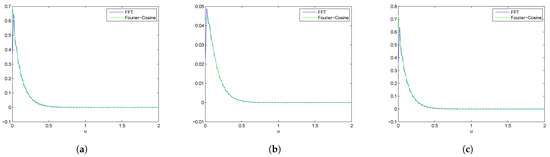
Figure 1.
For the Lévy-Gamma risk model, we compare Fourier–Cosine method with FFT method. (a) Ruin probability; (b) Expected claim size causing ruin; (c) Laplace transform of ruin time.
In the sequel, we consider the following cases,
with , respectively. To illustrate the performance of proposed estimator, 1000 sample paths of the risk process are generated and we use mean value and the integrated mean-square errors (IMSEs) for assessment purpose, which are computed by
where denotes the estimate in the j-th experiment. Since and are close to zero when , we calculate the integral in IMSEs on a finite domain .
First, we consider the case . To show variability bands and illustrate the stability of the procedures, we plot 25 consecutive estimate value curves and true value curves in Figure 2 for the compound Poisson risk model. It is clear that the estimates are very close to each other and close to the true value curves. Similarly, for the Lévy-Gamma risk model, we plot the estimate value curves and reference value curves in Figure 3 and we can obtain the same conclusion. Next, we present the mean value curves w.r.t. different pairs under both models in Figure 4 and Figure 5, respectively, and compare them with true/reference value curves. We find that our estimator performs very well and they converge to the true/reference value curves as increases. Let denote the standard derivation, which is computed by
Thereby, the confidence bands are constructed by
Then, we present the confidence bands in Figure 6 with for the L’evy-Gamma risk model, and we can observe that the confidence bands cover the reference value curves very well.
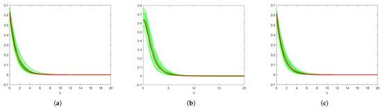
Figure 2.
For the compound Poisson risk model, we estimate the Gerber–Shiu functions by true value curves (red curves) and 25 estimated value curves (green curves). (a) Ruin probability; (b) Expected claim size causing ruin; (c) Laplace transform of ruin time.
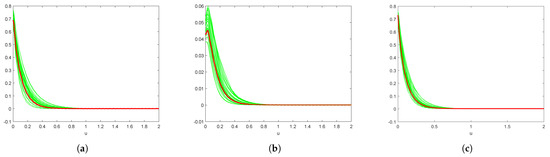
Figure 3.
For the Lévy-Gamma risk model, we estimate the Gerber–Shiu functions by true value curves (red curves) and 25 estimated value curves (green curves). (a) Ruin probability; (b) Expected claim size causing ruin; (c) Laplace transform of ruin time.
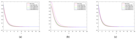
Figure 4.
For the compound Poisson risk model, we estimate the Gerber–Shiu functions by mean value curves. (a) Ruin probability; (b) Expected claim size causing ruin; (c) Laplace transform of ruin time.
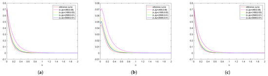
Figure 5.
For the Lévy-Gamma risk model, we estimate the Gerber–Shiu functions by mean value curves. (a) Ruin probability; (b) Expected claim size causing ruin; (c) Laplace transform of ruin time.
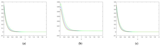
Figure 6.
For the Lévy-Gamma risk model, we plot the confidence band curves (green curves), mean value curves (blue curves) and reference value curves (red curves). (a) Ruin probability; (b) Expected claim size causing ruin; (c) Laplace transform of ruin time.
Finally, we compare the Fourier–Cosine method with FFT method in [18]. For the compound Poisson risk model, we report IMSEs in Table 1 for these two methods. It can be seen that Fourier–Cosine series expansion method has smaller IMSEs for each type of Gerber–Shiu function considered in the experiment. For the Lévy-Gamma risk model, corresponding IMSEs are displayed in Table 2 and we reach the same conclusion as for the compound Poisson risk model.

Table 1.
In the compound Poisson risk model, IMSEs for .
Table 2.
In the Lévy-Gamma risk model, IMSEs for .
5. Conclusions
In this paper, we estimate the Gerber–Shiu function under the Lévy risk model by Fourier–Cosine series expansion. Based on the high-frequency, discretely observed information, an estimator of the Gerber–Shiu function is constructed. We prove the consistency of the proposed estimator and test the performance of the estimator by some simulation examples when the sample size is finite. It is confirmed that our estimator is easy to compute and has a fast convergence rate. Further research on the asymptotic normality of the Fourier–Cosine series expansion remains open. The Fourier–Cosine method can be further extended to other risk models (e.g., Dividends, Capital injections) as well as economic models (e.g., Option pricing).
Author Contributions
Methodology, W.S., Y.W.; Software, W.S.; Writing—original draft, Y.W. Both authors have read and agreed to the published version of the manuscript.
Funding
The research of Wensu Su was supported by the National Natural Science Foundation of China (No. 11871121).
Institutional Review Board Statement
Not applicable.
Informed Consent Statement
Not applicable.
Data Availability Statement
The data in this paper are randomly generated and are not available for readers.
Conflicts of Interest
The authors declare no conflict of interest.
Appendix A
Proof.
For convenience, we define and
Then the triangle inequality gives
For the first term on the right hand side of (A1), we have
Note that for
then for the second term , we have
where we have used the following result,
Furthermore, using integration by parts, we have
As a result, (A3) gives
By (A4), the square of the third term on the right hand side of (A1) becomes
Since
we have
Combining (A1), (A2), (A5) and (A6) yields the result in Proposition 1. □
Appendix B
Proof.
First, for , the triangle inequality gives
For , it follows from Lemma A.3 in [18] that
which yields
For , we introduce two classes of real-valued functions,
where means taking imaginary part of a complex number. For any , we have
which implies that is contained the single bracket . Further, for two functions
with , we have
By the mean value theory, we have
where is a number between and . Then, inequality (A9) together with Assumption 6, gives
where . Under the Assumption 4, we have
due to Lemma 2. Hence, it follows from Example 19.7 in [41] that for every , the bracketing number satisfies
For every , the bracketing integral
Since under Assumption 4 ,
due to Lemma 2, then, by Corollary 19.35 in [41], we have
Similarly, we can obtain
Now we have
where the second step follows from (A10), (A11) and Markov’s inequality.
Appendix C
Proof.
By lemma A.5 in [18], we know that
where
First, by (A.13) in [18] we have
To study , we introduce the following classes of real-valued functions,
For any , we have
which implies that is contained in the single bracket . For two functions
with , by the mean value theory we have
Under Assumption 4 , it follows from Lemma 2 that
and
Hence, by exactly the same arguments in Lemma 3, we obtain
and
Further, together with Markov’s inequality, we have
References
- Lundberg, F. Approximerad Framställning av Sannolikhetsfunktionen. Aterforsdkerhlg av Kollektivrisk. Akad. Ph.D. Thesis, Afhandling, Almqvist och Wiksell, Uppsala, Sweden, 1903. [Google Scholar]
- Lundberg, F. Försäkringsteknisk Riskutjämning; F. Englunds Boktryckeri AB: Stockholm, Sweden, 1926. [Google Scholar]
- Gerber, H.U.; Shiu, E.S.W. On the time value of ruin. N. Am. Actuar. J. 1998, 2, 48–78. [Google Scholar] [CrossRef]
- Gerber, H.U. An extension of the renewal equation and its application in the collective theory of risk. Scand. Actuar. J. 1970, 1970, 205–210. [Google Scholar] [CrossRef]
- Tsai, C.C.L. On the expectations of the present values of the time of ruin perturbed by diffusion. Insur. Math. Econ. 2003, 32, 413–429. [Google Scholar] [CrossRef]
- Li, S.; Garrido, J. The Gerber-Shiu function in a Sparre Andersen risk process perturbed by diffusion. Scand. Actuar. J. 2005, 2005, 161–186. [Google Scholar] [CrossRef]
- Zhao, X.; Yin, C. The gerber-shiu expected discounted penalty function for Lévy insurance risk processes. Acta Math. Appl. Sin. Engl. Ser. 2010, 26, 575–586. [Google Scholar] [CrossRef]
- Kyprianou, A. Gerber-Shiu Risk Theory; Springer: Berlin/Heidelberg, Germany, 2013. [Google Scholar]
- Shimizu, Y. A new aspect of a risk process and its statistical inference. Insur. Math. Econ. 2009, 44, 70–77. [Google Scholar] [CrossRef]
- Shimizu, Y. Nonparametric estimation of the Gerber-Shiu function for the Winer-Poisson risk model. Scand. Actuar. J. 2012, 1, 56–69. [Google Scholar] [CrossRef]
- You, H.; Cai, C. Nonparametric estimation for a spectrally negative Lévy process based on high frequency data. J. Comput. Appl. Math. 2019, 345, 196–205. [Google Scholar] [CrossRef]
- You, H.L.; Yin, C.C. Threshold Estimation for a Spectrally Negative Lévy Process. Math. Probl. Eng. 2020, 6, 3561089. [Google Scholar] [CrossRef]
- You, H.L.; Guo, J.Y.; Jiang, J.C. Interval estimation of the ruin probability in the classical compound Poisson risk model. Comput. Stat. Dataan. 2020, 144, 106890. [Google Scholar] [CrossRef]
- You, H.L.; Gao, Y. Non-Parametric Threshold Estimation for the Wiener-Poisson Risk Model. Mathematics 2019, 7, 506. [Google Scholar] [CrossRef]
- Cai, C.H.; Chen, N.; You, H.L. Nonparametric estimation for a spectrally negative Lévy risk process based on low-frequency observation. J. Comput. Appl. Math. 2018, 328, 432–442. [Google Scholar] [CrossRef]
- Zhang, Z.M.; Yang, H. Nonparametric estimate of the ruin probability in a pure-jump Lévy risk model. Insur. Math. Econ. 2013, 53, 24–35. [Google Scholar] [CrossRef]
- Zhang, Z.M.; Yang, H. Nonparametric estimation for the ruin probability in a Lévy risk model under low-frequency observation. Insur. Math. Econ. 2014, 59, 168–177. [Google Scholar] [CrossRef]
- Shimizu, Y.; Zhang, Z. Estimating Gerber-Shiu functions from discretely observed Lévy driven surplus. Insur. Math. Econ. 2017, 74, 84–98. [Google Scholar] [CrossRef]
- Zhang, Z.M. Estimating the Gerber-Shiu function by Fourier-Sinc series expansion. Scand. Actuar. J. 2017, 10, 898–919. [Google Scholar] [CrossRef]
- Zhang, Z.M.; Su, W. A new efficient method for estimating the Gerber-Shiu function in the classical risk model. Scand. Actuar. J. 2018, 5, 426–449. [Google Scholar] [CrossRef]
- Su, W.; Yong, Y.; Zhang, Z.M. Estimating the Gerber-Shiu function in the perturbed compound Poisson model by Laguerre series expansion. J. Math. Anal. Appl. 2019, 469, 705–729. [Google Scholar] [CrossRef]
- Chau, K.; Yam, S.; Yang, H. Modern Fourier-cosine method for Gerber-Shiu function. Insur. Math. Econ. 2015, 61, 170–180. [Google Scholar] [CrossRef]
- Zhang, Z.M. Approximating the density of the time to ruin via Fourier-cosine series expansion. ASTIN Bull. 2017, 41, 169–198. [Google Scholar] [CrossRef]
- Fang, F.; Oosterlee, C.W. A novel pricing method for european options based on fourier-cosine series expansions. SIAM J. Sci. Comput. 2008, 31, 826–848. [Google Scholar] [CrossRef]
- Fang, F.; Oosterlee, C.W. Pricing early-exercise and discrete barrier options by fourier-cosine series expansions. Numer. Math. 2009, 114, 27–62. [Google Scholar] [CrossRef]
- Fang, F.; Oosterlee, C.W. A fourier-based valuation method for bermudan and barrier options under heston’s model. SIAM J. Financ. Math. 2011, 2, 439–463. [Google Scholar] [CrossRef]
- Ruijter, M.J.; Oosterlee, C.W. Two-dimensional Fourier cosine series expansion method for pricing financial options. SIAM J. Sci. Comput. 2012, 34, B642–B671. [Google Scholar] [CrossRef]
- Ruijter, M.J.; Oosterlee, C.W. A fourier cosine method for an efficient computation of solutions to BSDES. SIAM J. Sci. Comput. 2015, 37, A859–A889. [Google Scholar] [CrossRef]
- Ruijter, M.J.; Oosterlee, C.W. Numerical Fourier method and second-order Taylor scheme for backward SDEs in finance. Appl. Numer. Math. 2016, 103, 1–26. [Google Scholar] [CrossRef]
- Ruijter, M.J.; Oosterlee, C.W.; Aalbers, R.F.T. On the Fourier cosine series expansion method for stochastic control problems. Numer. Linear Algebr. 2013, 20, 598–625. [Google Scholar] [CrossRef]
- Kanemitsu, S.; Yoshimoto, M. Euler products, Farey series and the Riemann hypothesis. Publ. Math. 2000, 56, 431–449. [Google Scholar]
- Pellegrino, T.; Sabino, P. Pricing and hedging multiasset spread options using a three-dimensional Fourier cosine series expansion method. J. Energy. Mar. 2014, 7, 71–92. [Google Scholar] [CrossRef]
- Di Persio, L.; Pellegrini, G.; Bonollo, M. Polynomial chaos expansion approach to interest rate models. J. Probab. Stat. 2015, 2015, 369053. [Google Scholar] [CrossRef]
- Sun, Y.; Liu, C.; Guo, S. Stochastic volatility double-jump-diffusions model: The importance of distribution type of jump amplitude. Int. J. Comput. Math. 2017, 94, 989–1014. [Google Scholar] [CrossRef]
- Liang, C.; Li, S. Pricing and hedging European-style options in Lévy-based stochastic volatility models considering the leverage effect. J. Math. Anal. Appl. 2016, 438, 1010–1029. [Google Scholar] [CrossRef]
- Sun, X.; Gan, S.; Vanmaele, M. Analytical approximation for distorted expectations. Stat. Probabil. Lett. 2015, 107, 246–252. [Google Scholar] [CrossRef]
- Ruijter, M.J.; Oosterlee, C.W. The COS method for pricing options under uncertain volatility. In Topics in Numerical Methods for Finance; Springer: Boston, MA, USA, 2012; Volume 19, pp. 95–113. [Google Scholar]
- Marshall, S.L. On the analytical summation of Fourier series and its relation to the asymptotic behaviour of Fourier transforms. J. Phys. A Math. Gen. 1998, 31, 9957–9973. [Google Scholar] [CrossRef]
- Xie, J.; Zhang, Z. Finite-time dividend problems in a Lévy risk model under periodic observation. Appl. Math. Comput. 2021, 398, 125981. [Google Scholar]
- Comte, F.; Genon-Catalot, V. Nonparametric estimation for pure jump Lévy processes based on high frequency data. Stoch. Proc. Appl. 2009, 119, 4088–4123. [Google Scholar] [CrossRef][Green Version]
- Van der Vaart, A.W. Asymptotic Statistics; Cambridge University Press: Cambridge, UK, 1998. [Google Scholar]
Publisher’s Note: MDPI stays neutral with regard to jurisdictional claims in published maps and institutional affiliations. |
© 2021 by the authors. Licensee MDPI, Basel, Switzerland. This article is an open access article distributed under the terms and conditions of the Creative Commons Attribution (CC BY) license (https://creativecommons.org/licenses/by/4.0/).