A New Flexible Family of Continuous Distributions: The Additive Odd-G Family

Abstract

This paper introduces a new family of distributions based on the additive model structure. Three submodels of the proposed family are studied in detail. Two simulation studies were performed to discuss the maximum likelihood estimators of the model parameters. The log location-scale regression model based on a new generalization of the Weibull distribution is introduced. Three datasets were used to show the importance of the proposed family. Based on the empirical results, we concluded that the proposed family is quite competitive compared to other models.

1. Introduction

The main aim of generating new probability distributions is to increase the modeling ability of the baseline distribution. With this aim, many distribution generators have been introduced in the literature. Some well-known distribution generators are the Marshall–Olkin-G family [1], the beta-G family [2], the gamma-G family [3], the Kumaraswamy-G (Kw-G) family [4], the generalized beta-generated family [5], the T-X family [6], and the two-sided generalized family [7], among others. In addition to these families, many odd families of the distribution can be cited such as the odd log-logistic-G (OLL-G) family [8], the odd Weibull-G (OW-G) family [9], the odd Burr G family [10], the generalized odd log-logistic-G (GOLL-G) family [11], another generalized odd log-logistic-G (GOLL2-G) family [12], the odd log-logistic Lindley-G (OLLLi-G) family [13], the odd Chen-G (OCh-G) family [14], the odd flexible Weibull-H (OFW-H) family [15], and the new Kumaraswamy generalized (NKw-G) family [16]. These families bring more flexibility to the baseline model for data modeling.

To motivate the family in this paper, we considered a serial system with two independent components and supposed that the lifetime of the components follows the member of the OLL-G family and the member of the OW-G family with survival functions (sfs):

$$S_{OLL-G}\left(x;\alpha ,\theta \right)=\frac{\overline{G}{\left(x;\theta \right)}^{\alpha }}{G{\left(x;\theta \right)}^{\alpha }+\overline{G}{\left(x;\theta \right)}^{\alpha }}$$

(1)

and:

$$S_{OW-G}\left(x;\beta ,\theta \right)=exp\left\{-{\left(\frac{G\left(x;\theta \right)}{\overline{G}\left(x;\theta \right)}\right)}^{\beta }\right\},$$

(2)

respectively, where $x\in \Re$, $\alpha ,\beta >0$ are shape parameters, which control the tail, skewness, and kurtosis of the model, $G\left(x;\theta \right)$ is the baseline cumulative distribution function (cdf), $\theta$ is the parameter vector of the baseline distribution, and $\overline{G}\left(x;\theta \right)=1-G\left(x;\theta \right)$ is the sf of the baseline distribution. Hence, the sf of the system is given by:

$$S\left(x;\alpha ,\beta ,\theta \right)=\frac{\overline{G}{\left(x;\theta \right)}^{\alpha }}{G{\left(x;\theta \right)}^{\alpha }+\overline{G}{\left(x;\theta \right)}^{\alpha }}exp\left\{-{\left(\frac{G\left(x;\theta \right)}{\overline{G}\left(x;\theta \right)}\right)}^{\beta }\right\}.$$

(3)

With this definition in (3), we propose a new wider flexible family based on the OLL-G and the OW-G distributions by combining them in a serial system. The corresponding cdf and probability density function (pdf) of (3) are given by:

$$F\left(x;\alpha ,\beta ,\theta \right)=1-\frac{\overline{G}{\left(x;\theta \right)}^{\alpha }}{G{\left(x;\theta \right)}^{\alpha }+\overline{G}{\left(x;\theta \right)}^{\alpha }}exp\left\{-{\left(\frac{G\left(x;\theta \right)}{\overline{G}\left(x;\theta \right)}\right)}^{\beta }\right\}$$

(4)

and:

$$\begin{array}{c}\hfill f\left(x;\alpha ,\beta ,\theta \right)=\frac{g\left(x;\theta \right)\overline{G}{\left(x;\theta \right)}^{\alpha -1}}{G{\left(x;\theta \right)}^{\alpha }+\overline{G}{\left(x;\theta \right)}^{\alpha }}\left(\frac{\alpha G{\left(x;\theta \right)}^{\alpha -1}}{G{\left(x;\theta \right)}^{\alpha }+\overline{G}{\left(x;\theta \right)}^{\alpha }}+\frac{\beta G{\left(x;\theta \right)}^{\beta -1}}{\overline{G}{\left(x;\theta \right)}^{\beta }}\right)exp\left\{-{\left(\frac{G\left(x;\theta \right)}{\overline{G}\left(x;\theta \right)}\right)}^{\beta }\right\}\end{array}$$

(5)

respectively, where $g\left(x,\theta \right)$ is the baseline pdf.

The hazard rate function (hrf) of this family is given by:

$$\begin{array}{c}\hfill \tau \left(x;\alpha ,\beta ,\theta \right)=h\left(x;\theta \right)\left[\frac{\alpha G{\left(x;\theta \right)}^{\alpha -1}}{G{\left(x;\theta \right)}^{\alpha }+\overline{G}{\left(x;\theta \right)}^{\alpha }}+\frac{\beta G{\left(x;\theta \right)}^{\beta -1}}{\overline{G}{\left(x;\theta \right)}^{\beta }}\right]=h_{OLL-G}\left(x;\alpha ,\theta \right)+h_{OW-G}\left(x;\beta ,\theta \right),\end{array}$$

(6)

where $h\left(x;\theta \right)=\frac{g\left(x;\theta \right)}{\overline{G}\left(x;\theta \right)}$ is the hrf of the baseline distribution, $h_{OLL-G}\left(x;\alpha ,\theta \right)$ and $h_{OW-G}\left(x;\beta ,\theta \right)$ are the hrfs of the OLL-G and OW-G families, respectively. It can be seen that the cdf, pdf, and hrf of this family are the structure of the additive model with the OLL-G and OW-G families. The additive distribution models include the various pdf and hrf shapes for data modeling and ensure better fitting to the dataset than the ordinary distribution model. They are especially useful for lifetime data modeling since the empirical approaches to real data are often nonmonotone hrf. In general, there are many additive models based on the Weibull distribution in the literature such as the additive Weibull, by Xie and Lai [17], the additive Burr XII, by Wang [18], the modified Weibull, by Sarhan and Zaidin [19], the extended additive Weibull, by Almalki and Yuan [20], the log-logistic Weibull, by Oluyede et al. [21], and the additive modified Weibull distributions, by He et al. [22]. Therefore, we call this new family the additive odd log-logistic odd Weibull-G (AOLLOW-G) family and denote it by $AOLLOW$-$G(\alpha ,\beta ,\theta )$. We want to point out that the structure of the AOLLOW-G family can be proposed as a new method to obtain a flexible distribution family. As a real interpretation of the suggested model, consider a device with a two independent series subdevice with $Z_1\sim$ OLL-G and $Z_2\sim$ OW-G, then the lifetime of this device is $X=min\{Z_1,Z_2\}\sim$ AOLLOW-G, which is the suggested family. We were also motivated to introduce this family because it exhibits increasing, decreasing, constant, unimodal, unimodal, then bathtub, as well as bathtub hazard rates and its other shapes in modeling lifetime data.

The remaining parts of the study can be summarized as follows. Section 2 contains the special members of the proposed family. In Section 3, we present the linear combinations of the proposed family in terms of the exponentiated-G family. Section 4 contains the statistical properties. The parameter estimation issue of the proposed family is discussed in Section 5. The log location-scale regression model based on a new generalization of the Weibull distribution is introduced in Section 6. Two simulation studies related to the finite sample behavior of the estimators of the proposed model are given in Section 7. The empirical findings of the presented study are given in Section 8. The study is concluded in Section 9.

2. Special Members of the Family

The AOLLOW-G family generates alternative extended distributions, and it contains some new subfamilies. For example, the additive odd-log logistic odd exponential-G family is obtained for $\beta =1$, and the additive odd-log logistic odd Rayleigh-G family is obtained for $\beta =2$. It is reduced to the additive G odd Weibull-G family for $\alpha =1$, and it is the additive G odd exponential-G family for $\alpha =\beta =1$. It also is the additive G odd Rayleigh-G family for $\alpha =1$ and $\beta =2$. Now, we present the three important submodels of this new family.

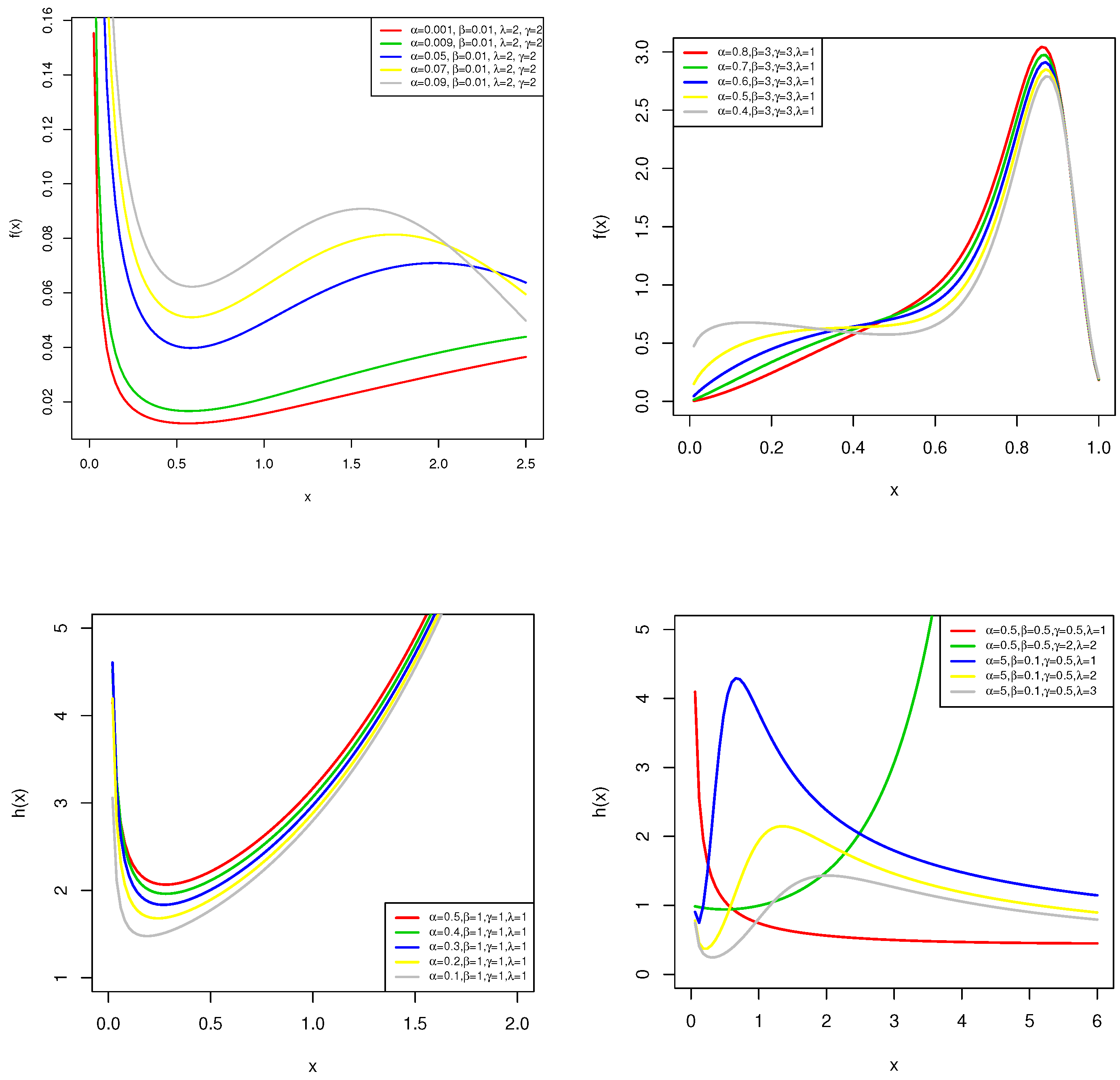
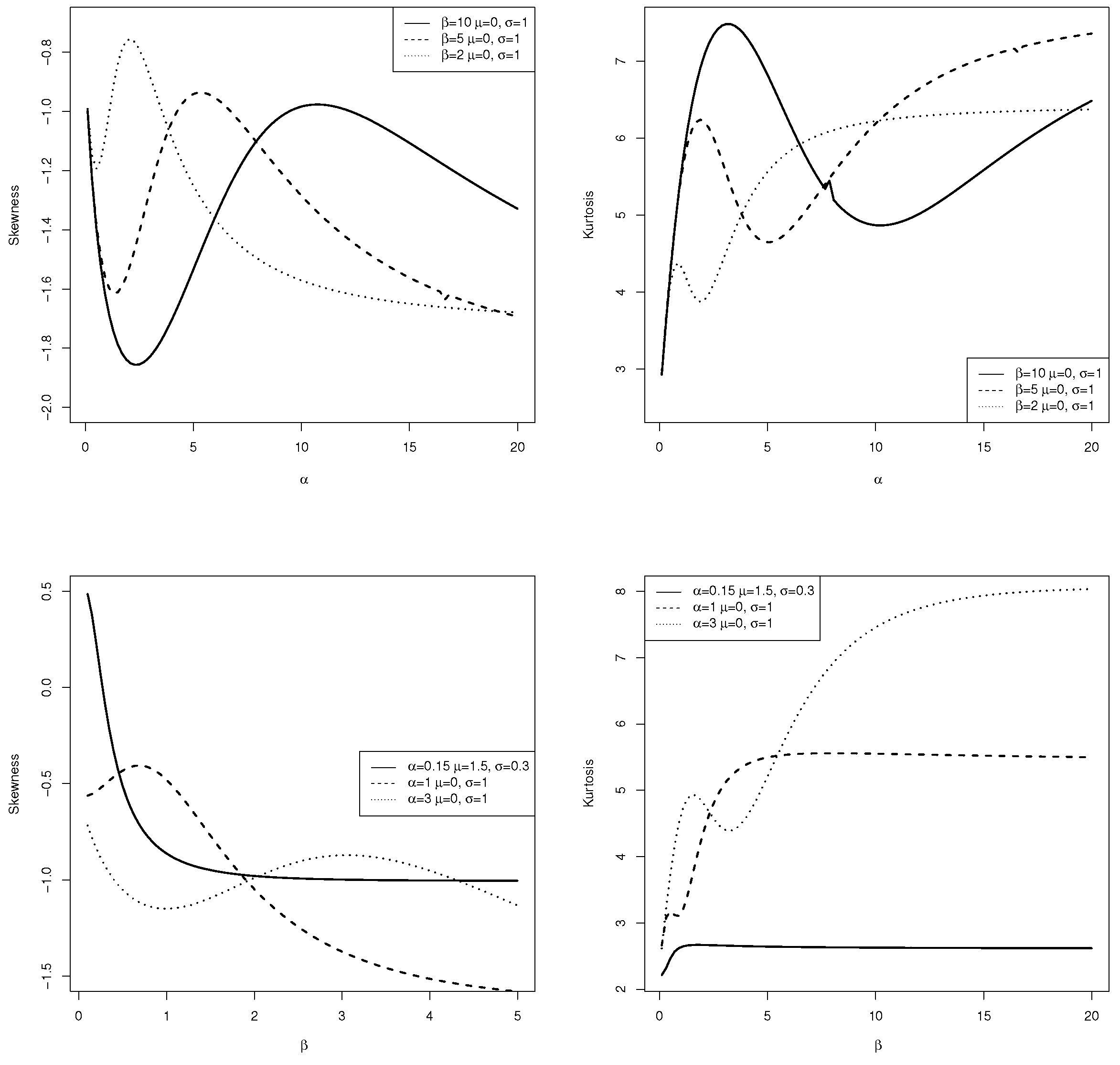
2.1. The AOLLOW-Normal Distribution

Let $G\left(x;\mu ,\sigma \right)=\Phi \left(\frac{x-\mu }{\sigma }\right)$ be the cdf of the normal distribution. The cdf of the AOLLOW-normal (AOLLOW-N) distribution is given by:

$$F\left(x;\alpha ,\beta ,\mu ,\sigma \right)=1-\frac{{\left[1-\Phi \left(\frac{x-\mu }{\sigma }\right)\right]}^{\alpha }}{\Phi {\left(\frac{x-\mu }{\sigma }\right)}^{\alpha }+{\left[1-\Phi \left(\frac{x-\mu }{\sigma }\right)\right]}^{\alpha }}exp\left\{-{\left(\frac{1}{\Phi \left(\frac{x-\mu }{\sigma }\right)}-1\right)}^{-\beta }\right\}.$$

Some possible plots of the AOLLOW-N density for selected parameter values are displayed in Figure 1. This figure shows that the pdf shapes of the AOLLOW-N can be trimodal, bimodal, unimodal, and skew-shaped. Therefore, we can say that new extended normal distribution has great flexible density shapes for data modeling.

Figure 1. The pdf plots of the AOLLOW-N distribution.

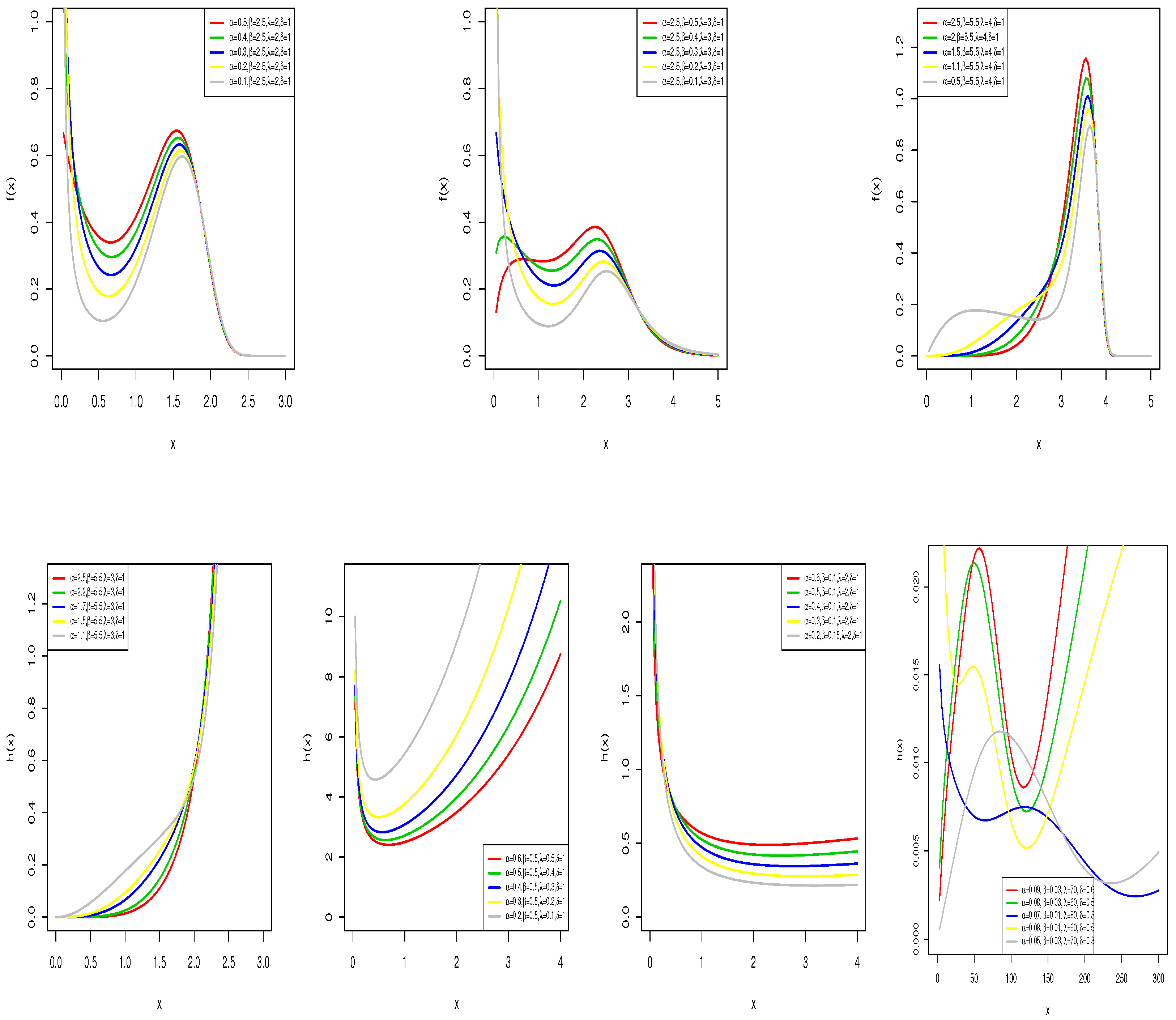
2.2. The AOLLOW-Weibull Distribution

Let $G\left(x;\lambda ,\gamma \right)=1-exp\left(-{\left(\lambda x\right)}^{\gamma }\right)$ be the cdf of the Weibull distribution with shape parameter $\gamma >0$ and scale parameter $\lambda >0$. The cdf of the AOLLOW-Weibull (AOLLOW-W) distribution is given by:

$$F\left(x;\alpha ,\beta ,\lambda ,\gamma \right)=1-\frac{e^{-\alpha {\left(\lambda x\right)}^{\gamma }}}{e^{-\alpha {\left(\lambda x\right)}^{\gamma }}+{\left(1-e^{-{\left(\lambda x\right)}^{\gamma }}\right)}^{\alpha }}exp\left\{-{\left(e^{{\left(\lambda x\right)}^{\gamma }}-1\right)}^{\beta }\right\}.$$

Figure 2 displays the pdf and hrf shapes of the AOLLOW-W. As seen from the figure, it is obvious that the AOLLOW-W distribution has left-right skewed and bimodal shapes. Its hrf structure is also very flexible and has the following shapes: increasing, decreasing, bathtub, decreasing-increasing-decreasing.

Figure 2. The pdf and hrf plots of the AOLLOW-W distribution.

The saturation characteristic of the AOLLOW-W distribution can be studied in the sense of the Hausdorff distance, which is important for reliability theory, financial mathematics, and debugging theory. This important property of the AOLLOW-W distribution is planned as a future work of the present study. Detailed information can be found in Kyurkchiev [23] and Kyurkchiev and Markov [24].

2.3. The AOLLOW-Gamma Distribution

Let $G\left(x;\delta ,\lambda \right)={\gamma }^{*}\left(\lambda ,\delta x\right){\Gamma }^{-1}\left(\lambda \right)$ be the cdf of the gamma distribution. The $\Gamma \left(·\right)$ is a complete gamma function, and ${\gamma }^{*}\left(\lambda ,\delta x\right)$ is defined as:

$${\gamma }^{*}\left(\lambda ,\delta x\right)={\int }_0^{\delta x}{t}^{\lambda -1}{e}^{-t}dt$$

which is called as incomplete gamma function. The cdf of the AOLLOW-gamma (AOLLOW-Ga) distribution is:

$$F\left(x;\alpha ,\beta ,\lambda ,\delta \right)=1-\frac{{\left[1-{\gamma }^{*}\left(\lambda ,\delta x\right){\Gamma }^{-1}\left(\lambda \right)\right]}^{\alpha }}{{\left[{\gamma }^{*}\left(\lambda ,\delta x\right){\Gamma }^{-1}\left(\lambda \right)\right]}^{\alpha }+{\left[1-{\gamma }^{*}\left(\lambda ,\delta x\right){\Gamma }^{-1}\left(\lambda \right)\right]}^{\alpha }}exp\left\{-{\left(\frac{{\gamma }^{*}\left(\lambda ,\delta x\right){\Gamma }^{-1}\left(\lambda \right)}{1-{\gamma }^{*}\left(\lambda ,\delta x\right){\Gamma }^{-1}\left(\lambda \right)}\right)}^{\beta }\right\}.$$

Figure 3 displays the pdf and hrf shapes of the AOLLOW-Ga distribution. We have the following results from these figures: (i) the pdf shapes of the AOLLOW-Ga distribution are left-right skewed and bimodal; (ii) the hrf shapes of the AOLLOW-Ga distribution are increasing, decreasing, bathtub, decreasing-increasing-decreasing-increasing, and increasing-decreasing-increasing. Since the new extended Weibull and gamma distributions have a very flexible density and hrf shapes, we can say that they can be useful especially in lifetime data modeling.

Figure 3. The pdf and hrf plots of the AOLLOW-Ga distribution.

3. Useful Expansions

Let us define the pdf and cdf of the exponentiated-G (exp-G) family for the parent distribution $G\left(x\right)$. The cdf and pdf of the exp-G family are given by:

$$\begin{array}{c}\hfill H_c\left(x\right)=G{\left(x\right)}^c,\end{array}$$

(7)

$$\begin{array}{c}\hfill h_c\left(x\right)=cg\left(x\right)G{\left(x\right)}^{c-1},\end{array}$$

(8)

The cdf of the AOLLOW-G family can be expressed as follows by using the generalized binomial expansion:

$$\begin{array}{ccc}\hfill F\left(x\right)& =& 1-\frac{\overline{G}{\left(x\right)}^{\alpha }}{G{\left(x\right)}^{\alpha }+\overline{G}{\left(x\right)}^{\alpha }}exp\{-{\left[\frac{G\left(x\right)}{\overline{G}\left(x\right)}\right]}^{\beta }\}\hfill \\ & =& 1-\frac{\overline{G}{\left(x\right)}^{\alpha }}{G{\left(x\right)}^{\alpha }+\overline{G}{\left(x\right)}^{\alpha }}\sum _{l=0}^{\infty }\frac{{(-1)}^l}{l!}{\left[\frac{G\left(x\right)}{\overline{G}\left(x\right)}\right]}^{\beta l}\hfill \\ & =& 1-\sum _{l,j=0}^{\infty }\frac{{(-1)}^{l+j}{(\alpha -\beta l)}_j}{l!}\frac{G{\left(x\right)}^{\beta l+j}}{G{\left(x\right)}^{\alpha }+\overline{G}{\left(x\right)}^{\alpha }}\hfill \end{array}$$

(9)

The second part of (9) can be written as follows:

$$\begin{array}{c}\hfill \frac{G{\left(x\right)}^{\beta l+j}}{G{\left(x\right)}^{\alpha }+\overline{G}{\left(x\right)}^{\alpha }}=\frac{{\sum }_{k=0}^{\infty }{b}_{k}G{\left(x\right)}^k}{{\sum }_{k=0}^{\infty }{a}_{k}G{\left(x\right)}^k}=\sum _{k=0}^{\infty }{c}_{k}G{\left(x\right)}^k\end{array}$$

(10)

where:

$$\begin{array}{ccc}& & a_k=\sum _{i=k}^{\infty }{(-1)}^{i+k}\left({\displaystyle \genfrac{}{}{0pt}{}{\beta l+j}{i}}\right)\left({\displaystyle \genfrac{}{}{0pt}{}{i}{k}}\right)\hfill \\ & & b_k={(-1)}^k\left({\displaystyle \genfrac{}{}{0pt}{}{\alpha }{k}}\right)+\sum _{i=k}^{\infty }{(-1)}^{i+k}\left({\displaystyle \genfrac{}{}{0pt}{}{\alpha }{i}}\right)\left({\displaystyle \genfrac{}{}{0pt}{}{i}{k}}\right)\hfill \end{array}$$

(11)

$$c_0=\frac{a_0}{b_0}$$

For $k\ge 1$,

$$\begin{array}{c}\hfill c_k=\frac{1}{b_0}\left[a_k-\frac{1}{b_0}\sum _{r=1}^k{b}_r{c}_{k-r}\right]\end{array}$$

(12)

Then, we can write:

$$\begin{array}{ccc}\hfill F\left(x\right)& =& 1-\sum _{k=0}^{\infty }{w}_{k}G{\left(x\right)}^k=\sum _{k=0}^{\infty }{d}_{k}G{\left(x\right)}^k=\sum _{k=0}^{\infty }{d}_k{H}_k\left(x\right)\hfill \end{array}$$

(13)

where $w_k={\sum }_{l,j=0}^{\infty }\frac{{(-1)}^{l+j}{(\alpha -\beta l)}_j}{l!}{c}_k(\alpha ,\beta ,l,j)$, $d_0=1-w_0$, and for $k\ge 1$, $d_k=-w_k$.

$H_k\left(x\right)=G{\left(x\right)}^k$ denotes the exp-G with power parameter k.

We can write:

$$\begin{array}{ccc}\hfill f\left(x\right)& =& \sum _{k=0}^{\infty }{d}_{k+1}{h}_{k+1}\left(x\right)\hfill \end{array}$$

(14)

and $h_{k+1}\left(x\right)=(k+1)g\left(x\right)G{\left(x\right)}^k$ denote the pdf of the exp-G with power parameter $k+1$. The main result of this section is (14), which shows that the proposed family can be expressed as a linear combination of the exp-G densities. This property of the proposed family helps us obtain its statistical properties based on the exp-G densities.

4. Statistical Properties

This section deals with the statistical properties of the proposed family.

4.1. Quantile Function

Generating random variables from continuous probability distributions is generally performed by the quantile function (qf). The uth quantile, denoted by $x_u=Q\left(u\right)$, of the AOLLOW-G distribution is obtained by the solution of the equation:

$$log\left[\left(1-u\right)\left({\left[\frac{G\left(x_u;\theta \right)}{\overline{G}\left(x_u;\theta \right)}\right]}^{\alpha }+1\right)\right]-{\left[\frac{G\left(x_u;\theta \right)}{\overline{G}\left(x_u;\theta \right)}\right]}^{\beta }=0,$$

(15)

where $u\in \left(0,1\right)$. We can also write for the qf of any AOLLOW-G distribution:

$$\begin{array}{c}\hfill x_u=min\{Q_G(\frac{u_{}^{1/\alpha }}{u_{}^{1/\alpha }+{(1-u_{})}^{1/\alpha }}),Q_G(\frac{(-log{(1-u))}^{1/\beta }}{1+(-log{(1-u))}^{1/\beta }})\},\end{array}$$

(16)

where $Q_G(.)=G^{-1}(.)$ denotes the qf of the G baseline distribution and $u\in \left(0,1\right)$. Using (15) or (16), the random variables can be generated from any member of the proposed family.

4.2. Moments

Let $Y_k$ follow an exp-G distribution with the parameter $k+1$. Using (14), the nth moment of the AOLLOW-G family is:

$$\begin{array}{c}\hfill {\displaystyle E\left(X^n\right)=\sum _{k=0}^{\infty }{d}_{k+1}E\left(Y_k^n\right).}\end{array}$$

(17)

Regarding the moments of exp-G distributions, one can visit the work of Nadarajah and Kotz [25].

Equation (17) can be expressed based on the G qf as follows:

$$\begin{array}{c}\hfill {\displaystyle E\left(X^n\right)=\sum _{k=0}^{\infty }(k+1)d_{k+1}\tau (n,k),}\end{array}$$

(18)

where $\tau (n,k)={\int }_{-\infty }^{\infty }{x}^{n}G{\left(x\right)}^{k}g\left(x\right)dx={\int }_0^1{Q}_G{\left(u\right)}^n{u}^{k}du$. Cordeiro and Nadarajah [26] provided an explicit expression for $\tau (n,k)$ for some beta generalized distributions.

For integer values of n, let ${\mu }_n^{{}^{\prime }}=E\left(X^n\right)$ and $\mu ={\mu }_1^{{}^{\prime }}=E\left(X\right)$, then one can also find the nth central moment of the AOLLOW-G distribution as:

$$\begin{array}{c}\hfill {\mu }_n=E{(X-\mu )}^n=\sum _{i=0}^n\left(\genfrac{}{}{0pt}{}{n}{i}\right){\mu }_i^{{}^{\prime }}{(-\mu )}^{n-i}.\end{array}$$

(19)

Using (19), we calculate the skewness and kurtosis of the AOLLOW-G as follows:

$$Skewness\left(X\right)=\frac{\mu {{}^{\prime }}_3-3\mu {{}^{\prime }}_2\mu {{}^{\prime }}_1+2\mu {{}^{\prime }}_1^3}{{\left(\mu {{}^{\prime }}_2-\mu {{}^{\prime }}_1^2\right)}^{\frac{3}{2}}},$$

(20)

and:

$$Kurtosis\left(X\right)=\frac{\mu {{}^{\prime }}_4-4{\mu }_1^{{}^{\prime }}\mu {{}^{\prime }}_3+6\mu {{}^{\prime }}_1^2\mu {{}^{\prime }}_3-3\mu {{}^{\prime }}_1^4}{\mu {{}^{\prime }}_2-\mu {{}^{\prime }}_1^2},$$

(21)

respectively. Figure 4 displays the skewness and kurtosis plots of the AOLLOW-N distribution. These figures help us to understand how additional shape parameters affect the shape of the distribution.

Figure 4. The skewness and kurtosis plots for the selected AOLLOW-N distributions.

4.3. Generating Function

Let $M_X\left(t\right)=E\left({\mathrm{e}}^{\mathrm{t}\mathrm{X}}\right)$ where $X\sim$ AOLLOW-G, then the first one simply comes from (14) as:

$$\begin{array}{c}\hfill {\displaystyle M_X\left(t\right)=\sum _{k=0}^{\infty }{d}_{k+1}{M}_k\left(t\right),}\end{array}$$

(22)

where $M_k\left(t\right)$ is the moment generating function (mgf) of $Y_k$. So, exp-G generating function is used to obtain $M_X\left(t\right)$. From (14), we have:

$$\begin{array}{c}\hfill {\displaystyle M\left(t\right)=\sum _{i=0}^{\infty }(k+1)d_{k+1}\rho (t,k),}\end{array}$$

(23)

where $\rho (t,k)={\int }_{-\infty }^{\infty }{\mathrm{e}}^{\mathrm{t}\mathrm{x}}\mathrm{G}{\left(\mathrm{x}\right)}^{\mathrm{k}}\mathrm{g}\left(\mathrm{x}\right)\mathrm{dx}={\int }_0^{1}exp\left[\mathrm{t}{\mathrm{Q}}_{\mathrm{G}}\left(\mathrm{u}\right)\right]{\mathrm{u}}^{\mathrm{k}}\mathrm{du}$.

Equation (23) can be used to obtain the mgfs of the different distributions obtained by means of the AOLLOW-G family.

5. Inference

The unknown parameters of the AOLLOW-G family are estimated by means of the maximum likelihood estimation (MLE) method. Let $\Psi =$($\alpha ,\beta ,{\theta }^{⊺}$)${}^{⊺}$ be an unknown parameter vector where $\theta$ is a $q\times 1$ parameter vector for the baseline distribution. Under these settings, the log-likelihood function of the AOLLOW-G family is:

$$\begin{array}{ccc}\hfill \ell & & =\sum _{i=1}^{n}logg\left(x_i;\theta \right)+\left(\alpha -1\right)\sum _{i=1}^{n}log\overline{G}\left(x_i;\theta \right)-\sum _{i=1}^{n}log\left[G{\left(x_i;\theta \right)}^{\alpha }+\overline{G}{\left(x_i;\theta \right)}^{\alpha }\right]\hfill \\ & & -\sum _{i=1}^{n}log\left[\frac{\alpha G{\left(x_i;\theta \right)}^{\alpha -1}}{G{\left(x_i;\theta \right)}^{\alpha }+\overline{G}{\left(x_i;\theta \right)}^{\alpha }}+\frac{\beta G{\left(x_i;\theta \right)}^{\beta -1}}{\overline{G}{\left(x_i;\theta \right)}^{\beta }}\right]-\sum _{i=1}^n{\left(\frac{G\left(x_i;\theta \right)}{\overline{G}\left(x_i;\theta \right)}\right)}^{\beta }.\hfill \end{array}$$

(24)

One could prefer to obtain the score vectors corresponding to the likelihood function, given in (24). To do this, it is necessary to take partial derivatives of (24) with respect to the parameters such as $U\left(\Psi \right)=\frac{\partial \ell }{\partial \Psi }={(\frac{\partial \ell }{\partial \alpha },\frac{\partial \ell }{\partial \beta },\frac{\partial \ell }{\partial {\theta }_q})}^{⊺}$. The simultaneous solution of these score vectors gives the MLE of the unknown parameter vector, $\Psi$. Note that the score vectors can be requested from the authors. Unfortunately, it is impossible to obtain the explicit solution of these nonlinear equation systems. Therefore, the log-likelihood has to be maximized by using the optimization algorithms. Here, we prefer the optim function of the R software for this purpose. The asymptotic confidence intervals of the parameters are constructed based on the observed information matrix.

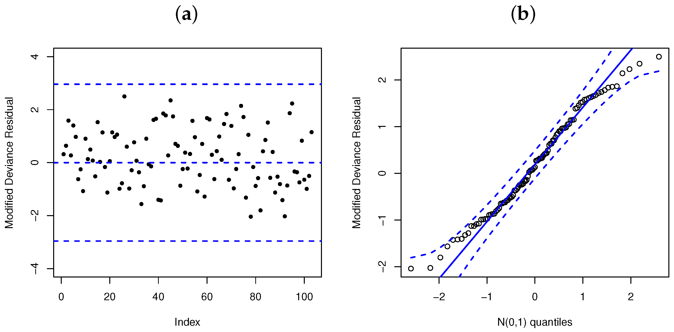
6. Regression Modeling

In this section, a new location-scale regression model is introduced based on the AOLLOW-W distribution. For this aim, we use the log-transformation and some convenient parametrizations on the AOLLOW-W distribution. Let $\gamma =1/\sigma$ and $\lambda =exp\left(-\mu \right)$ and $Y=log\left(X\right)$. We have the following density for the random variable Y:

$$\begin{array}{c}f\left(y\right)=\frac{\frac{1}{\sigma }exp\left[\left(\frac{y-\mu }{\sigma }\right)-exp\left(\frac{y-\mu }{\sigma }\right)\right]{\left(exp\left[-exp\left(\frac{y-\mu }{\sigma }\right)\right]\right)}^{\alpha -1}}{{\left\{1-exp\left[-exp\left(\frac{y-\mu }{\sigma }\right)\right]\right\}}^{\alpha }+{\left(exp\left[-exp\left(\frac{y-\mu }{\sigma }\right)\right]\right)}^{\alpha }}\hfill \\ \times \left(\frac{\alpha {\left\{1-exp\left[-exp\left(\frac{y-\mu }{\sigma }\right)\right]\right\}}^{\alpha -1}}{{\left\{1-exp\left[-exp\left(\frac{y-\mu }{\sigma }\right)\right]\right\}}^{\alpha }+{\left(exp\left[-exp\left(\frac{y-\mu }{\sigma }\right)\right]\right)}^{\alpha }}+\frac{\beta {\left\{1-exp\left[-exp\left(\frac{y-\mu }{\sigma }\right)\right]\right\}}^{\beta -1}}{{\left(exp\left[-exp\left(\frac{y-\mu }{\sigma }\right)\right]\right)}^{\beta }}\right)\hfill \\ \times exp\left\{-{\left(\frac{\left\{1-exp\left[-exp\left(\frac{y-\mu }{\sigma }\right)\right]\right\}}{exp\left[-exp\left(\frac{y-\mu }{\sigma }\right)\right]}\right)}^{\beta }\right\}\hfill \end{array},$$

(25)

where $y\in \Re$. The parameters $\mu \in \Re$ and $\sigma >0$ are the location and scale parameters, respectively. The parameters $\alpha >0$ and $\beta >0$ are the shape parameters. The density in (25) is denoted as Y ∼ LAOLLOW-W $(\alpha ,\beta ,\sigma ,\mu )$. The pdf shapes of the LAOLLOW-W distribution are displayed in Figure 5, which shows that the LAOLLOW-W can be used to model different types of the datasets such as left-skewed, symmetric, and bimodal shapes.

Figure 5. The pdf plots of the LAOLLOW-W density.

The sf is:

$$S\left(y\right)=\frac{{\left(exp\left[-exp\left(\frac{y-\mu }{\sigma }\right)\right]\right)}^{\alpha }}{{\left\{1-exp\left[-exp\left(\frac{y-\mu }{\sigma }\right)\right]\right\}}^{\alpha }+{\left(exp\left[-exp\left(\frac{y-\mu }{\sigma }\right)\right]\right)}^{\alpha }}exp\left\{-{\left(\frac{\left\{1-exp\left[-exp\left(\frac{y-\mu }{\sigma }\right)\right]\right\}}{\left(exp\left[-exp\left(\frac{y-\mu }{\sigma }\right)\right]\right)}\right)}^{\beta }\right\}.$$

(26)

Besides, using the standardized random variable, $Z=(Y-\mu )/\sigma$, we have:

$$\begin{array}{c}f\left(z\right)=\frac{exp\left[z-exp\left(z\right)\right]{\left(exp\left[-exp\left(z\right)\right]\right)}^{\alpha -1}}{{\left\{1-exp\left[-exp\left(z\right)\right]\right\}}^{\alpha }+{\left(exp\left[-exp\left(z\right)\right]\right)}^{\alpha }}\hfill \\ \times \left(\frac{\alpha {\left\{1-exp\left[-exp\left(z\right)\right]\right\}}^{\alpha -1}}{{\left\{1-exp\left[-exp\left(z\right)\right]\right\}}^{\alpha }+{\left(exp\left[-exp\left(z\right)\right]\right)}^{\alpha }}+\frac{\beta {\left\{1-exp\left[-exp\left(z\right)\right]\right\}}^{\beta -1}}{{\left(exp\left[-exp\left(z\right)\right]\right)}^{\beta }}\right)\hfill \\ \times exp\left\{-{\left(\frac{\left\{1-exp\left[-exp\left(z\right)\right]\right\}}{exp\left[-exp\left(z\right)\right]}\right)}^{\beta }\right\}\hfill \end{array}.$$

(27)

Now, using the LAOLLOW-W density, we introduce a location-scale regression model by linking the covariates to the location of the random variable Y by means of the identity link function. Consider the regression structure:

$$y_i={\mathbf{x}}_i^{\top }\mathit{\beta }+\sigma z_i,\mathrm{i}=1,\dots ,\mathrm{n},$$

(28)

where ${\mathit{x}}_i^{\top }=\left(x_{i1},\dots ,x_{ik}\right)$ is the independent variable vector and $y_i$ is the dependent variable, following the density in (25). The regression parameters are represented by the vector, $\mathit{\beta }={({\beta }_1,\dots ,{\beta }_k)}^{\top }$. The dependent variable is defined as $y_i=min\{log\left(t_i\right),log\left(c_i\right)\}$ where $t_i$ and $c_i$ are the observed lifetime and censoring times, respectively. Let F and C be the sets representing the lifetime and censoring times. Based on these specifications, the log-likelihood function of the LAOLLOW-W regression model is:

$$\begin{array}{c}\ell \left(\tau \right)=-rlog\left(\sigma \right)+{\displaystyle \sum _{i\in F}}\left(z_i-u_i\right)-\left(\alpha -1\right){\displaystyle \sum _{i\in F}}{u}_i-{\displaystyle \sum _{i\in F}}log\left[{\left\{1-exp\left[-u_i\right]\right\}}^{\alpha }+{\left(exp\left[-u_i\right]\right)}^{\alpha }\right]\hfill \\ +{\displaystyle \sum _{i\in F}}log\left(\frac{\alpha {\left\{1-exp\left[-u_i\right]\right\}}^{\alpha -1}}{{\left\{1-exp\left[-u_i\right]\right\}}^{\alpha }+{\left(exp\left[-u_i\right]\right)}^{\alpha }}+\frac{\beta {\left\{1-exp\left[-u_i\right]\right\}}^{\beta -1}}{{\left(exp\left[-u_i\right]\right)}^{\beta }}\right)-{\displaystyle \sum _{i\in F}}{\left(\frac{\left\{1-exp\left[-u_i\right]\right\}}{exp\left[-u_i\right]}\right)}^{\beta }\hfill \\ -\alpha {\displaystyle \sum _{i\in C}}{u}_i-{\displaystyle \sum _{i\in C}}log\left[{\left\{1-exp\left[-u_i\right]\right\}}^{\alpha }+{\left(exp\left[-u_i\right]\right)}^{\alpha }\right]-{\displaystyle \sum _{i\in C}}{\left(\frac{\left\{1-exp\left[-u_i\right]\right\}}{\left(exp\left[-u_i\right]\right)}\right)}^{\beta }\hfill \end{array},$$

(29)

where $\mathit{\tau }=\left(\alpha ,\beta ,\sigma ,\mathit{\beta }\right)$, $u_i=exp\left(z_i\right)$ and $z_i=(y_i-x_i^{\top }\mathit{\beta })/\sigma$. Note that r is the number of uncensored observations. The MLE of the unknown parameter vector, $\widehat{\mathit{\tau }}$, is obtained based on the maximization of the given log-likelihood function in (29). The optim function of the R software is used to minimize the negative log-likelihood function. The standard errors of the estimated parameters are obtained by means of observed information, which is easily obtained by the Hess function of the R software.

Residual Analysis

Residual analysis is required to control the accuracy of the proposed regression model for the fitted dataset. For this goal, we consider two residuals. These are the martingale and modified deviance residuals. The martingale residual (see Fleming and Harrington [27]) of the LAOLLOW-W model is given by:

$$r_{M_i}=\left\{\begin{array}{c}1+log\left(\frac{{\left(exp\left[-u_i\right]\right)}^{\alpha }}{{\left\{1-exp\left[-u_i\right]\right\}}^{\alpha }+{\left(exp\left[-u_i\right]\right)}^{\alpha }}exp\left\{-{\left(\frac{\left\{1-exp\left[-u_i\right]\right\}}{\left(exp\left[-u_i\right]\right)}\right)}^{\beta }\right\}\right)\mathrm{if}i\in F,\hfill \\ log\left(\frac{{\left(exp\left[-u_i\right]\right)}^{\alpha }}{{\left\{1-exp\left[-u_i\right]\right\}}^{\alpha }+{\left(exp\left[-u_i\right]\right)}^{\alpha }}exp\left\{-{\left(\frac{\left\{1-exp\left[-u_i\right]\right\}}{\left(exp\left[-u_i\right]\right)}\right)}^{\beta }\right\}\right)\mathrm{if}i\in C,\hfill \end{array}\right.$$

(30)

Since the martingale residuals are not distributed symmetrically, its interpretation has some difficulties. In this case, the modified deviance residuals, proposed by Therneau et al. [28], are generally used, which are defined as:

$$r_{D_i}=\left\{\begin{array}{c}\mathrm{sign}\left(r_{M_i}\right){\left\{-2\left[r_{M_i}+log\left(1-r_{M_i}\right)\right]\right\}}^{1/2},\mathrm{if}i\in F\hfill \\ \mathrm{sign}\left(r_{M_i}\right){\left\{-2r_{M_i}\right\}}^{1/2},\mathrm{if}i\in C,\hfill \end{array}\right.$$

(31)

where ${\widehat{r}}_{M_i}$ is the martingale residual.

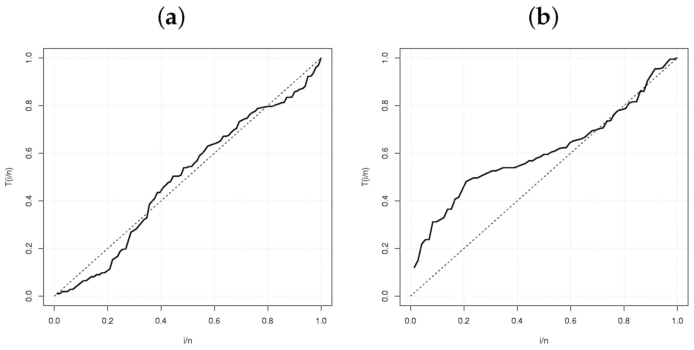
7. Simulation Studies

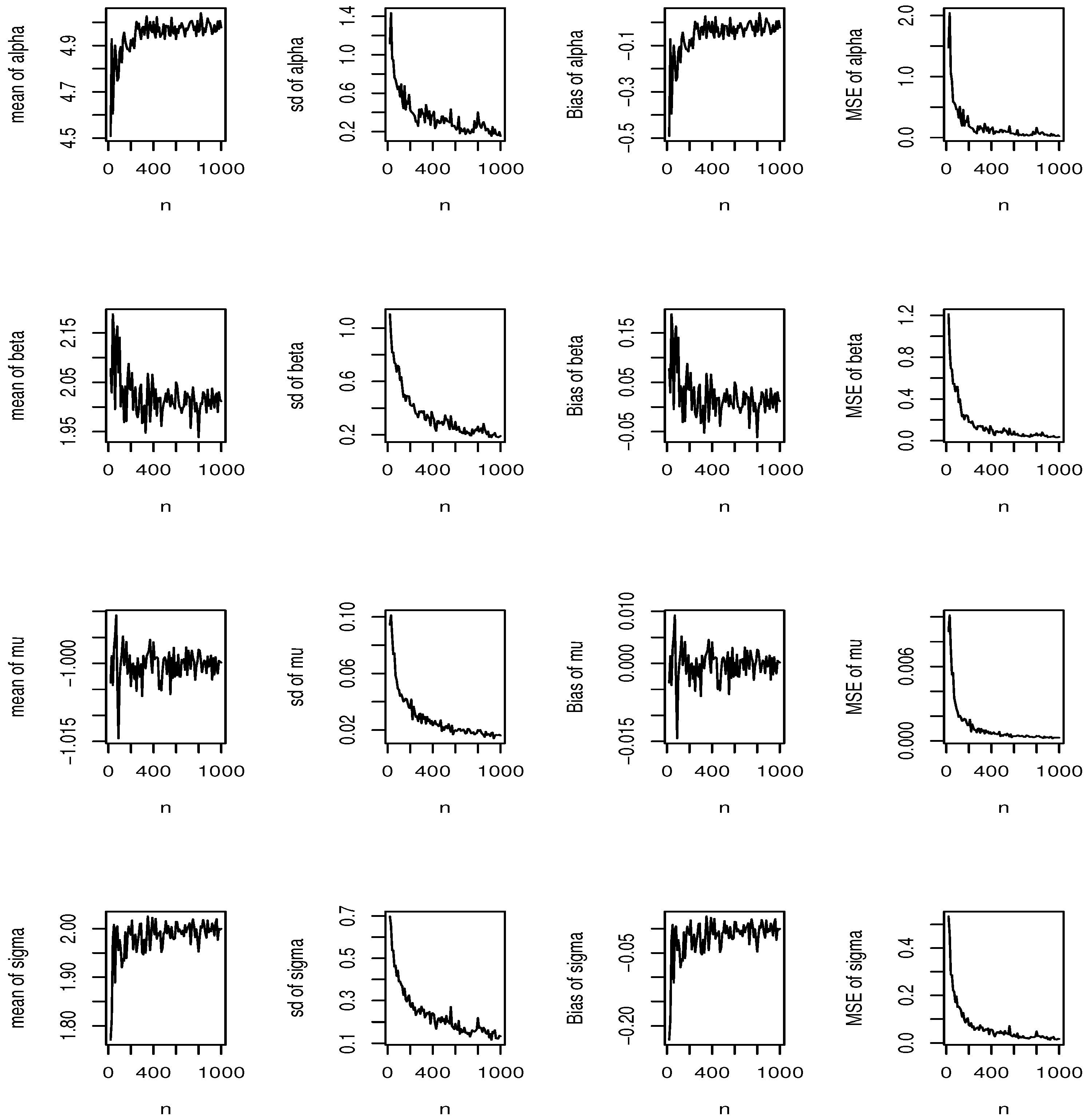
7.1. Simulation Study 1

The AOLLOW-N distribution was used for the first simulation. The simulation was repeated $N=1000$ times. The sample size was increased by 10 units such as $n=20,30,\dots ,1000$. The parameter values were $\alpha =5$, $\beta =2$, $\mu =-1$, and $\sigma =2$. The results were evaluated based on the following metrics: estimated mean, bias, standard deviation (sd), and mean squared error (MSE). Our expectation was to see that when n is sufficiently large, the estimated biases and MSEs should be near the zero. The simulation results, displayed in Figure 6, verified our expectation. Therefore, the MLE method is the preferable method to obtain the unknown parameters of the AOLLOW-N distribution.

Figure 6. Simulation results of the AOLLOW-N distribution.

7.2. Simulation Study 2

The AOLLOW-W distribution was used for the second simulation. As in the first simulation, the simulation replication number was $N=1000$. The sample sizes used were: $n=20,60,100$. The results are discussed based on the estimated mean and sd of the MLEs. Table 1 contains the simulation results. The results in this table show that the estimated mean and sd decrease withthe sample size n.

Table 1. The simulation results of the AOLLOW-W distribution based on empirical mean and standard deviation (in parentheses).

Parameters	$\mathit{n}=20$				$\mathit{n}=60$				$\mathit{n}=100$
$\mathit{\alpha },\mathit{\beta },\mathit{\lambda },\mathit{\gamma }$	$\widehat{\mathit{\alpha }}$	$\widehat{\mathit{\beta }}$	$\widehat{\mathit{\lambda }}$	$\widehat{\mathit{\gamma }}$	$\widehat{\mathit{\alpha }}$	$\widehat{\mathit{\beta }}$	$\widehat{\mathit{\lambda }}$	$\widehat{\mathit{\gamma }}$	$\widehat{\mathit{\alpha }}$	$\widehat{\mathit{\beta }}$	$\widehat{\mathit{\lambda }}$	$\widehat{\mathit{\gamma }}$
0.5, 2, 0.5, 2	0.5327	2.0754	0.5156	2.1858	0.5076	2.0187	0.5060	2.0686	0.5067	2.0205	0.5022	2.0351
	(0.2003)	(0.4328)	(0.0359)	(0.3527)	(0.0982)	(0.2422)	(0.0174)	(0.2160)	(0.0717)	(0.1615)	(0.0125)	(0.1509)
1, 0.5, 0.5, 2	1.0407	0.5491	0.5232	2.5367	1.0167	0.5465	0.5040	2.1541	1.0018	0.5399	0.5016	2.1123
	(0.6327)	(0.2974)	(0.0848)	(0.7923)	(0.4233)	(0.1849)	(0.0428)	(0.5598)	(0.3554)	(0.1624)	(0.0330)	(0.4873)
5, 5, 0.5, 0.5	4.9099	5.0724	0.5266	0.5407	4.8526	5.0990	0.5177	0.5245	4.9784	5.0163	0.5074	0.5098
	(0.3564)	(0.2439)	(0.0797)	(0.1098)	(0.5727)	(0.4224)	(0.0490)	(0.0624)	(0.1569)	(0.1126)	(0.0343)	(0.0419)
2, 2, 2, 2	1.8851	2.3515	2.0364	2.2521	1.9740	2.1548	2.0125	2.0790	1.9996	2.0880	2.0051	2.0457
	(0.7248)	(0.5187)	(0.1201)	(0.5273)	(0.5768)	(0.3070)	(0.0661)	(0.2762)	(0.5067)	(0.0661)	(0.0547)	(0.2370)
1, 2, 3, 4	1.1058	2.1757	3.0427	4.3521	1.0355	2.0483	3.0127	4.1308	1.0216	2.0211	3.0075	4.0867
	(0.4546)	(0.7245)	(0.0893)	(0.5841)	(0.2447)	(0.3964)	(0.0516)	(0.3320)	(0.2018)	(0.3024)	(0.0407)	(0.2894)
4, 3, 2, 1	3.8858	3.0293	2.1136	1.2596	3.9176	3.0012	2.0539	1.1167	3.9575	2.9717	2.0368	1.0697
	(0.7970)	(0.9388)	(0.2442)	(0.5369)	(0.6317)	(0.7288)	(0.1538)	(0.2735)	(0.4844)	(0.5696)	(0.1172)	(0.1893)

8. Data Analysis

Three datasets were analyzed to compare the special cases of the AOLLOW-G family with existing models such as the Kw-G, GOLL-G, GOLL2-G, OLL-G, OW-G, and additive Weibull (AW) by Lemonte et al. [29]. The information criteria and goodness-of-fit test below were used to select the best model for the modeled data:

• Akaike information criterion (AIC);
• Kolmogorov–Smirnov (KS);
• Cramer–von Mises ($W^{*}$);
• Anderson–Darling ($A^{*}$).

Furthermore, the estimated log-likelihood values $\widehat{\ell }$ were used to select the best model. See Chen and Balakrishnan [30] for detailed information on $W^{*}$ and $A^{*}$. The smallest values of these metrics show the best model for the data. Additionally, we used the total time on test (TTT) plot (Aarset [31]) to determine the shape of the empirical hrf. The TTT plots of the two datasets are given in Figure 7.

Figure 7. TTT plots for stress data (a) and guinea pig data (b).

8.1. Stress Data

The data regarded the stress-rupture life of Kevlar 49/epoxy strands. Andrews and Herzberg [32], Cooray and Ananda [33], and Paraniaba et al. [34] analyzed the same dataset. Figure 7a shows that the empirical hrf of the data has a convex-concave-convex shape. Table 2 contains the estimated parameters, as well as goodness-of-fit statistics. From these results, we concluded that the AOLLOW-W distribution is the best choice among the others since it had the lowest values of the model selection criteria.

Table 2. The results of the first data set (standard errors of the estimates are in parentheses).

Model	$\widehat{\mathit{\alpha }}$	$\widehat{\mathit{\beta }}$	$\widehat{\mathit{\lambda }}$	$\widehat{\mathit{\gamma }}$	$-\widehat{\mathit{\ell }}$	$\mathbf{AIC}$	$\mathbf{KS}$	${\mathit{A}}^{*}$	${\mathit{W}}^{*}$
AOLLOW-W	43.5199	10.9591	0.0002	0.04619	99.9641	207.9282	0.0505	0.3790	0.0460
	(10.6311)	(1.6396)	(0.00001)	(0.0017)
AW	0.6703	0.7893	0.3139	1.2451	102.8146	213.6292	0.0826	0.9372	0.1601
	(0.7347)	(0.2712)	(0.7209)	(0.5576)
GOLL2-W	0.8891	0.6399	1.6166	1.0111	102.8434	213.6869	0.0902	1.0140	0.1814
	(0.1949)	(0.1222)	(0.2645)	(0.1777)
GOLL-W	1.1712	0.6062	0.6131	1.1123	102.7667	213.5335	0.0798	0.9348	0.1561
	(0.9348)	(0.8847)	(0.9732)	(0.4377)
Kw-W	0.7197	0.2429	3.5048	1.0362	102.6217	213.2433	0.0752	0.8432	0.1376
	(0.0053)	(0.0245)	(0.0041)	(0.0106)
OLL-W	0.8892		1.0396	1.0109	102.8435	211.6869	0.0903	1.0145	0.1816
	(0.1944)		(0.1286)	(0.1771)
OW-W		6.2492	0.0330	0.1077	102.8714	211.7428	0.0847	0.9778	0.1686
		(13.8005)	(0.2478)	(0.2391)
W			1.0101	0.9260	102.9768	209.9536	0.0906	1.1220	0.1963
			(0.1141)	(0.0726)

Figure 8 gives information about the suitability of the fitted distributions for the dataset graphically. From these figures, one can conclude that the AOLLOW-W distribution is a good choice for the data used. Additionally, only the estimated hrf of the AOLLOW-W overlaps with the result of the TTT plot.

Figure 8. The fitted plots for the first dataset.

8.2. Guinea Pig Data

The second dataset regarded the survival times (in days) of guinea pigs (Bjerkedal [35]). Gupta et al. [36], Korkmaz and Genç [37], and Korkmaz [38] analyzed the same dataset with various probability distributions. Figure 7b shows that the empirical hrf of the data is concave-convex-concave.

The estimated parameters and goodness-of-fit test results are given in Table 3. As in the previous application, the proposed model, AOLLOW-Ga, had the lowest values of the model selection criteria. Moreover, to strengthen the suitability of the AOLLOW-Ga distribution for the data, the fitted functions of the AOLLOW-Ga and other competitive distributions are plotted in Figure 9. It is obvious that the AOLLOW-Ga distribution is the best among the others and provided a nearly perfect fit to the data.

Table 3. The results of the second data set (standard errors of the estimates are in parentheses).

Model	$\widehat{\mathit{\alpha }}$	$\widehat{\mathit{\beta }}$	$\widehat{\mathit{\delta }}$	$\widehat{\mathit{\lambda }}$	$-\widehat{\mathit{\ell }}$	$\mathbf{AIC}$	$\mathbf{KS}$	${\mathit{A}}^{*}$	${\mathit{W}}^{*}$
AOLLOW-Ga	0.0598	0.0371	0.4412	74.2805	386.5875	781.1751	0.0883	0.5483	0.1003
	(0.0163)	(0.0057)	($2.3\times {10}^{-6}$)	(1.1 × 10−9)
GOLL2-Ga	4.5123	3.4472	$7.7\times {10}^{-5}$	3.5404	391.0022	790.0043	0.0897	0.9138	0.1411
	(1.3647)	(2.5399)	($1\times {10}^{-6}$)	(0.1279)
GOLL-Ga	12.2028	0.0621	$1.7\times {10}^{-5}$	1.6275	390.5474	789.0948	0.0906	0.7493	0.1254
	(1.1728)	(0.0403)	(0.0001)	(0.9773)
Kw-Ga	287.2096	0.3796	0.0306	0.0206	390.3771	788.7543	0.0986	0.9409	0.1761
	(0.4384)	(0.1826)	(0.0140)	(0.0099)
OLL-Ga	10.3182		$2.5\times {10}^{-5}$	0.1202	390.6752	787.3503	0.0888	0.8285	0.1285
	(0.7899)		(0.0001)	(0.1771)
OW-Ga		0.0465	0.3925	61.1120	394.4674	794.9348	0.2276	5.2988	1.1630
		(0.0042)	(0.0001)	(0.1688)
Ga			0.0208	2.0810	394.2476	792.4952	0.1385	1.8960	0.3555
			(0.0037)	(0.3232)

Figure 9. The fitted plots for the second dataset.

8.3. Stanford Heart Transplant Dataset

In the third application, the practicability of the LAOLLOW-W regression model was discussed based on the real data. Brito et al. [39] used the Stanford heart transplant dataset for the log-Topp–Leone odd log-logistic-Weibull (Log-TLOLL-W) regression model. We used the same dataset to compare the proposed model with the log-TLOLL-W model. The total individuals were $n=103$, and the percentage of the censored observations was 27%. The dependent variable survival time $y_i$ was modeled with the following covariates:

✓

$x_1$: year of acceptance to the program;

✓

$x_2$: age of the patient (years);

✓

$x_3$: previous surgery $\left(1=yes,0=no\right)$;

✓

$x_4$: transplant $\left(1=yes,0=no\right)$.

We consider the regression structure:

$$y_i={\beta }_0+{\beta }_1{x}_{i1}+{\beta }_2{x}_{i2}+{\beta }_3{x}_{i3}+{\beta }_4{x}_{i4}+\sigma z_i,$$

(32)

The above regression structure is fit by the log-Weibull, log-TLOLL-W, and log-AOLLOW-W models. The results of the fitted regression models are summarized in Table 4, giving the estimated parameters, standard errors, p-values, and the the model selection AIC and BIC. From these results, we concluded that the LAOLLOW-W regression model is the best choice among the others for the dataset used. The regression parameters, ${\beta }_1$ and ${\beta }_2$ were found to be statistically significant at the 1% level. Therefore, the survival time increased when the year of acceptance increased. Besides, when the age of the patient increased, the survival time decreased.

Table 4. The results of the fitted regression models.

Models
	Log-Weibull			Log-TLOLL-W			LAOLLOW-W
Parameters	Estimate	S.E.	p-Value	Estimate	S.E.	p-Value	Estimate	S.E.	p-Value
$\alpha$	-	-	-	2.340	3.546	-	5.244	4.840	-
$\beta$	-	-	-	24.029	3.015	-	4.986	5.745	-
$\sigma$	1.478	0.133	-	9.680	12.526	-	8.270	8.640	-
${\beta }_0$	1.639	6.835	0.811	−0.645	8.459	0.939	6.689	3.199	0.036
${\beta }_1$	0.104	0.096	0.279	0.074	0.097	0.448	0.236	0.086	0.006
${\beta }_2$	−0.092	0.02	<0.001	−0.053	0.02	0.009	−0.079	0.018	<0.001
${\beta }_3$	1.126	0.658	0.087	1.676	0.597	0.005	−0.082	0.470	0.861
${\beta }_4$	2.544	0.378	<0.001	2.394	0.384	<0.001	0.263	0.355	0.458
$-\ell$	171.2405			164.684			161.911
AIC	354.481			345.368			339.822
BIC	370.2894			366.4458			360.900

Model Accuracy

The accuracy of the fitted regression model was checked using the modified deviance residuals. Figure 10 displays the index and quantile–quantile (qq) plots. The expectation was that when the fitted model is statistically valid, the modified deviance residuals should be distributed as N(0,1). From the qq plot, it is easy to conclude that the LAOLLOW-W regression model is statistically valid. The index plot of the modified deviance residuals shows that there were no observations evaluated as possible outliers.

Figure 10. The index (a) and qq (b) plots of the modified deviance residuals.

9. Concluding Remark

A new family of distributions was introduced with two extra shape parameters. The mathematical properties were studied in detail. Simulation studies were implemented. The location-scale regression model was also introduced. Three datasets were analyzed. The empirical results showed that the AOLLOW-G family gives better results than other famous G-families of distributions. As a future work of the present paper, we plan to develop a bivariate version of the AOLLOW-G family. Furthermore, this family can be used to generate new heavy-tailed distributions by using the Pareto as a baseline distribution. A new generalization of the Pareto distribution using the proposed family can be applied to financial datasets to forecast financial risk. We hope that this new family captures many application areas.

References

- Marshall, A.W.; Olkin, I. A new method for adding a parameter to a family of distributions with application to the exponential and Weibull families. Biometrika 1997, 84, 641–652. [Google Scholar] [CrossRef]
- Eugene, N.; Lee, C.; Famoye, F. Beta-normal distribution and its applications. Commun. Stat. Theory Methods 2002, 31, 497–512. [Google Scholar] [CrossRef]
- Zografos, K.; Balakrishnan, N. On families of beta-and generalized gamma-generated distributions and associated inference. Stat. Methodol. 2009, 6, 344–362. [Google Scholar] [CrossRef]
- Cordeiro, G.M.; Castro, M. A new family of generalized distributions. J. Stat. Comput. Simul. 2011, 81, 883–898. [Google Scholar] [CrossRef]
- Alexander, C.; Cordeiro, G.M.; Ortega, E.M.; Sarabia, J.M. Generalized beta-generated distributions. Comput. Stat. Data Anal. 2012, 56, 1880–1897. [Google Scholar] [CrossRef]
- Alzaatreh, A.; Lee, C.; Famoye, F. A new method for generating families of continuous distributions. Metron 2013, 71, 63–79. [Google Scholar] [CrossRef] [Green Version]
- Korkmaz, M.Ç.; Genç, A.I. A new generalized two-sided class of distributions with an emphasis on two-sided generalized normal distribution. Commun. Stat. Simul. Comput. 2017, 46, 1441–1460. [Google Scholar] [CrossRef]
- Gleaton, J.U.; Lynch, J.D. Properties of generalized log-logistic families of lifetime distributions. J. Probab. Stat. Sci. 2006, 4, 51–64. [Google Scholar]
- Bourguignon, M.; Silva, R.B.; Cordeiro, G.M. The Weibull-G family of probability distributions. J. Data Sci. 2014, 12, 53–68. [Google Scholar] [CrossRef]
- Alizadeh, M.; Cordeiro, G.M.; Nascimento, A.D.; Lima, M.D.C.S.; Ortega, E.M. Odd-Burr generalized family of distributions with some applications. J. Stat. Comput. Simul. 2017, 87, 367–389. [Google Scholar] [CrossRef]
- Cordeiro, G.M.; Alizadeh, M.; Ozel, G.; Hosseini, B.; Ortega, E.M.M.; Altun, E. The generalized odd log-logistic family of distributions: Properties, regression models and applications. J. Stat. Comput. Simul. 2017, 87, 908–932. [Google Scholar] [CrossRef]
- Haghbin, H.; Ozel, G.; Alizadeh, M.; Hamedani, G.G. A new generalized odd log-logistic family of distributions. Commun. Stat. Theory Methods 2017, 46, 9897–9920. [Google Scholar] [CrossRef]
- Alizadeh, M.; Afify, A.Z.; Eliwa, M.S.; Ali, S. The odd log-logistic Lindley-G family of distributions: Properties, Bayesian and non-Bayesian estimation with applications. Comput. Stat. 2020, 35, 281–308. [Google Scholar] [CrossRef]
- El-Morshedy, M.; Eliwa, M.S.; Afify, A.Z. The odd Chen generator of distributions: Properties and estimation methods with applications in medicine and engineering. J. Natl. Sci. Found. Sri Lanka 2020, 48, 113–130. [Google Scholar]
- El-Morshedy, M.; Eliwa, M.S. The odd flexible Weibull-H family of distributions: Properties and estimation with applications to complete and upper record data. Filomat 2019, 33, 2635–2652. [Google Scholar] [CrossRef]
- Tahir, M.H.; Hussain, M.A.; Cordeiro, G.M.; El-Morshedy, M.; Eliwa, M.S. A new Kumaraswamy generalized family of distributions with properties, applications, and bivariate extension. Mathematics 2020, 8, 1989. [Google Scholar] [CrossRef]
- Xie, M.; Lai, C.D. Reliability analysis using an additive Weibull model with bathtub-shaped failure rate function. Reliabil. Eng. Syst. Saf. 1996, 52, 87–93. [Google Scholar] [CrossRef]
- Wang, F.K. A new model with bathtub-shaped failure rate using an additive Burr XII distribution. Reliabil. Eng. Syst. Saf. 2000, 70, 305–312. [Google Scholar] [CrossRef]
- Sarhan, A.M.; Zaindin, M. Modified Weibull distribution. Appl. Sci. 2009, 11, 123–136. [Google Scholar]
- Almalki, S.J.; Yuan, J. A new modified Weibull distribution. Reliabil. Eng. Syst. Saf. 2013, 111, 164–170. [Google Scholar] [CrossRef]
- Oluyede, B.; Foya, S.; Warahena-Liyanage, G.; Huang, S. The log-logistic weibull distribution with applications to lifetime data. Aust. J. Stat. 2016, 45, 43–69. [Google Scholar] [CrossRef]
- He, B.; Cui, W.; Du, X. An additive modified Weibull distribution. Reliabil. Eng. Syst. Saf. 2016, 145, 28–37. [Google Scholar] [CrossRef]
- Kyurkchiev, N. Comments on the epsilon and omega cumulative distributions: “Saturation in the hausdorff sense”. AIP Conf. Proc. 2021, 2321, 030020-1–030020-8. [Google Scholar]
- Kyurkchiev, N.; Markov, S. On the Hausdorff distance between the Heaviside step function and Verhulst logistic function. J. Math. Chem. 2016, 54, 109–119. [Google Scholar] [CrossRef]
- Nadarajah, S.; Kotz, S. The exponentiated-type distributions. Acta Appl. Math. 2006, 92, 97–111. [Google Scholar] [CrossRef]
- Cordeiro, G.M.; Nadarajah, S. Closed-form expressions for moments of a class of beta generalized distributions. Braz. J. Probab. Stat. 2011, 25, 14–33. [Google Scholar] [CrossRef]
- Fleming, T.R.; Harrington, D.P. Counting Process and Survival Analysis; John Wiley: New York, NY, USA, 1994. [Google Scholar]
- Therneau, T.M.; Grambsch, P.M.; Fleming, T.R. Martingale-based residuals for survival models. Biometrika 1990, 77, 147–160. [Google Scholar] [CrossRef]
- Lemonte, A.J.; Cordeiro, G.M.; Ortega, E.M. On the additive Weibull distribution. Commun. Stat. Theory Methods 2014, 43, 2066–2080. [Google Scholar] [CrossRef]
- Chen, G.; Balakrishnan, N. A general purpose approximate goodness-of-fit test. J. Qual. Technol. 1995, 27, 154–161. [Google Scholar] [CrossRef]
- Aarset, M.V. How to identify a bathtub hazard rate. IEEE Trans. Reliabil. 1987, 36, 106–108. [Google Scholar] [CrossRef]
- Andrews, D.F.; Herzberg, A.M. Data: A Collection of Problems from Many Fields for the Student and Research Worker; Springer: New York, NY, USA, 1985. [Google Scholar]
- Cooray, K.; Ananda, M.M. A generalization of the half-normal distribution with applications to lifetime data. Commun. Stat. Theory Methods 2008, 37, 1323–1337. [Google Scholar] [CrossRef]
- Paranaiba, P.F.; Ortega, E.M.; Cordeiro, G.M.; Pascoa, M.A.D. The Kumaraswamy Burr XII distribution: Theory and practice. J. Stat. Comput. Simul. 2013, 83, 2117–2143. [Google Scholar] [CrossRef]
- Bjerkedal, T. Acquisition of resistance in guinea pigs infected with different doses of virulent tubercle bacilli. Am. J. Hyg. 1960, 72, 130–148. [Google Scholar] [PubMed]
- Gupta, R.C.; Kannan, N.; Raychaudhuri, A. Analysis of lognormal survival data. Math. Biosci. 1997, 139, 103–115. [Google Scholar] [CrossRef]
- Korkmaz, M.Ç.; Genç, A.I. Two-Sided Generalized Exponential Distribution. Commun. Stat. Theory Methods 2015, 44, 5049–5070. [Google Scholar] [CrossRef]
- Korkmaz, M.Ç. A generalized skew slash distribution via gamma-normal distribution. Commun. Stat. Simul. Comput. 2017, 46, 1647–1660. [Google Scholar] [CrossRef]
- Brito, E.; Cordeiro, G.M.; Yousof, H.M.; Alizadeh, M.; Silva, G.O. The Topp Leone odd log-logistic family of distributions. J. Stat. Comput. Simul. 2017, 87, 3040–3058. [Google Scholar] [CrossRef]
Publisher’s Note: MDPI stays neutral with regard to jurisdictional claims in published maps and institutional affiliations. |
© 2021 by the authors. Licensee MDPI, Basel, Switzerland. This article is an open access article distributed under the terms and conditions of the Creative Commons Attribution (CC BY) license (https://creativecommons.org/licenses/by/4.0/).