Multi-Objective Optimization of Plastics Thermoforming

Abstract

The practical application of a multi-objective optimization strategy based on evolutionary algorithms was proposed to optimize the plastics thermoforming process. For that purpose, in this work, differently from the other works proposed in the literature, the shaping step was considered individually with the aim of optimizing the thickness distribution of the final part originated from sheets characterized by different thickness profiles, such as constant thickness, spline thickness variation in one direction and concentric thickness variation in two directions, while maintaining the temperature constant. As far we know, this is the first work where such a type of approach is proposed. A multi-objective optimization strategy based on Evolutionary Algorithms was applied to the determination of the final part thickness distribution with the aim of demonstrating the validity of the methodology proposed. The results obtained considering three different theoretical initial sheet shapes indicate clearly that the methodology proposed is valid, as it provides solutions with physical meaning and with great potential to be applied in real practice. The different thickness profiles obtained for the optimal Pareto solutions show, in all cases, that that the different profiles along the front are related to the objectives considered. Also, there is a clear improvement in the successive generations of the evolutionary algorithm.

1. Introduction

Thermoforming is a thermoplastic processing technique commonly used in the rigid packaging industry. A variety of thermoplastic materials can be used in this process, including semi-crystalline polymers, such as High Density Polyethylene (HDPE) and Polypropylene (PP) and amorphous polymers, such as Acrylonitrile Butadiene Styrene (ABS), Polystyrene (PS) and High Impact Polystyrene (HIPS). HIPS is a lightweight and inexpensive thermoplastic often used in thermoformed food and pharmaceutical packaging containers.

Thermoforming comprises a sequence of interdependent operations and is characterized by being sensitive to the intrinsic properties of thermoplastics, namely the lower heat conduction and the deformation capability strongly dependent on temperature. In general, the thermoforming comprises: a heating stage, which aims to allow the sheet to acquire the required deformability; a sheet deformation stage in order to reproduce the contours of the piece and finally, a cooling stage, which allows the part to be extracted from the mold without distorting. In this way, the final performance of thermoformed products results from the sum of all actions that occur in these three main stages. Since there are processing variables associated with each of the three stages, including the material properties as a function of temperature, optimizing the thermoforming process is a complex task.

Generally, the optimization of thermoforming, like in the other real word optimization problems, consists of relating the effect of the operating variables of each stage with the performance of the part. Since thermoformed parts are characterized by having a non-uniform thickness that can hinder their performance, the thickness distribution of the final part is one of the most used variables to characterize the performance of the part. Furthermore, the effects of processing parameters on the thermoforming of polymeric sheets are highly nonlinear and fully coupled, which increases the difficulty of the process design. The following studies aim at optimizing the sheet deformation stage with the objective of obtaining thermoformed parts with the most uniform thickness distribution.

Yang and Hung [1] proposed an inverse Artificial Neural Network (ANN) with the aim of predicting the optimum processing conditions (decision variables), including sheet temperature, vacuum pressure, plug speed and displacement inside the mold. The network inputs are the thickness distribution at different positions of molded PET parts, and the outputs are the processing conditions obtained by the ANN presented, which show a good agreement between the computed result and experimental data. However, the ANN was trained using experimental data and the authors were not clear about the optimization method used. Also, the fact that different inputs for this inverse ANN can produce identical results at the output side was not discussed.

Chang et al. [2] used a similar inverse ANN to obtain the optimal processing parameters of polypropylene foam thermoforming. The studied variables included the mold temperature, plug speed and displacement, vacuum pressure and time and the heat transfer coefficient of the plug. Experimental data from tests carried out on a lab-scale thermoforming machine were used to train the ANN, used as an inverse model of the process. Product dimensions were used as the inverse model inputs and the corresponding processing parameters as outputs. The feasibility of the proposed method was demonstrated by experimental manufacturing of cups with optimal geometry derived from the computational method. In almost all points, the deviations between predicted and measured points were all below 3.5%. Like in the previous paper, the authors did not take into account that different inputs can produce identical results.

Leite et al. [3,4] developed models to predict and optimize the thermoforming using ANN defining the processing parameters set as the networks’ inputs and deviations in part thickness as the outputs. For the ANN data, thermoformed samples were experimentally produced using a 1 mm polystyrene sheet, using a fractional factorial design (2^k−p). The studied processing variables included heating time and the electric heating power of the heater panel vacuum time pressure. Preliminary computational studies were carried out with various ANN structures and configurations with the test data, until reaching satisfactory models and, afterward, multi-criteria optimization models were developed. The validation tests were developed with the models’ predictions and solutions showed that the estimates for them have prediction errors within the limit of values found in the samples produced. Thus, it was demonstrated that, within certain limits, the ANN models are valid to simulate the vacuum thermoforming process using multiple parameters, decision variables and objectives, by means of reduced data quantity.

Sasimowski [5] used experimental data to determine a utility function by regression analysis in order to calculate the thickness distribution of the thermoformed parts. This utility function was used to optimize the operating conditions of the machine, namely heating time, heater temperature, pre-blow time, vacuum time and cooling time. In all of these works, the ANN was used to predict the behavior evolution of the thermoformed parts thickness during information. Thus, no specific optimization method was described/applied to optimize the results that the trained ANN predicted, being these modeling results were used to optimize the process based on empirical knowledge.

In all of these works, it was not clear what is the optimization method used. In fact, ANN is not an optimization method by itself, but a way of predicting output values from a set of input data, obtained experimentally or computationally, very similar to a regression model. The ANN, in the present context, works as a modeling program with the aim of predicting the process performance. To optimize the process, it is necessary to link a modeling routine with an optimization method through an optimization methodology able to deal with the objectives to be optimized, as will be described in Section 3. Additionally, most of these works are based on experimental data, which makes the process unrealistic given the time required to do the experiments.

In addition to the general studies on the optimization of thermoforming, it is possible to find in the literature studies aiming at controlling the different stages of the process, namely the heating and forming stages.

Regarding the heating stage, the main objective is controlling the sheet temperature and the temperature fields developing during this step. This is very complex since the heating methods are indirect, that is, the sheet temperature is controlled by adjusting the heaters variables, and not directly. Furthermore, determining an optimum processing window in thermoforming process with the aim of achieving high quality parts is critical. In practice, the infrared heating stage is crucial since the final thickness distribution of the thermoformed part is closely related to the temperature of the sheet.

Wang and Nied [6] used a numerical approach based on the finite element method to obtain inverse solutions for the thermoforming processes. This was done by specifying a desired final thickness distribution and iteratively solving the system for the temperature field needed to obtain the desired result. A uniform initial temperature distribution is used as the initial guess for the iterative optimization procedure. Subsequently, updated non-uniform initial temperatures are obtained, based on the complete process of simulation for achieving the final thickness distribution during thermoforming. Suitable inverse solutions are achieved once the desired thickness distribution is obtained within a specified tolerance. The sensitivity of final part thickness to perturbations in temperature distribution is also investigated and shown to be a potential problem for precise thickness control in industrial applications.

Bordival et al. [7] developed an automatic optimization method of the ovens geometric parameters to be used in thermoforming. The first time, a simple analytical model, coupled to a nonlinear constraint optimization method (Sequential Quadratic Programming) allows one to find the best set of parameters, according to a cost function representing, for example, the heat flux uniformity. Then, with these optimized parameters, an accurate raytracing method is used to compute the irradiation resulting from the interaction between lamps and the thermoplastic sheet. Finally, a control volume method is implemented to solve the three-dimensional transient heat transfer equation, where the radiation source is approximated by a diffusion Rosseland model.

Chy and co-authors [8,9] presented a method to control the surface temperature of a plastic sheet using model predictive control (MPC) to solve the inverse heating problem (IHP). The model was implemented on a complex thermoforming oven with a large number of inputs and outputs for precise control of sheet temperatures under hard constraints on heater temperature and their rates. Even though the MPC controller can handle a multivariable process, the large number of computations makes it difficult to apply to large systems such as multi-zone temperature control in a thermoforming machine.

Li and co-authors [10,11] suggested a methodology to compute and optimize the sheet temperature by controlling the heater temperature. The steady-state optimum distribution of heater power is first ascertained by a numerical optimization to obtain a uniform sheet temperature. The time-dependent optimal heater input is then determined to decrease the temperature difference through the direction of the thickness using the response surface method and the D-optimal method. The results show that the time-dependent optimum heater power distribution gives an acceptable uniform sheet temperature in the forming temperature range by the end of the heating process.

More recently, Erchiqui and co-authors [12,13,14,15] proposed the application of two different meta-heuristic algorithms, Simulated Annealing (SA) and Evolutionary Algorithms (EA) to detect, from a fixed and random set of temperatures of the radiant zones of the oven, the best temperatures that must be assigned to the heating zones in order to ensure a uniform sheet temperature. For numerical heating analysis, the nonlinear heat conduction problem is solved by a specific 3D volumetric enthalpy-based computational method.

However, these studies only considered the effects of the heating phase on the final thickness distribution of the thermoformed parts, having a starting point a sheet with constant thickness, that is, the aim is to determine how to heat the different zones of the sheet in order to induce uniform thickness on the final part.

Furthermore, an important limitation of the methodologies proposed in the literature lies in the fact that the process is intrinsically multi-objective, and the different stages cannot be considered independent. In reality, the results of one stage of the process depend strongly on the remaining stages, the final part thickness distribution does not depend only on the heating, but also on the initial thickness of the sheet used. Therefore, the main aim of the work is to apply multi-objective strategies to optimize the plastics thermoforming process. The intention is to propose a more global methodology that can take into account the different steps and characteristics of this process, as described in the next section. However, due to its complexity, only the stage of the sheet deformation will be considered here. More specifically, the aim is to study the influence of the initial sheet thickness distribution on the optimization of the process. For that purpose, three different initial thickness distribution sheets will be considered. As far as we know, there is no work in the literature that addresses the problem from this point of view. From an industrial perspective, the fabrication of the sheets to be thermoformed must be changed if economic and/or environmental gains can be obtained.

The paper is organized as follows: in Section 2 the details of thermoforming related to optimization are explained, Section 3 addresses the concepts of multi-objective optimization and the algorithm used, in Section 4 the results and discussion for the optimization of thermoforming are presented and in Section 5 the conclusions are stated.

2. Thermoforming

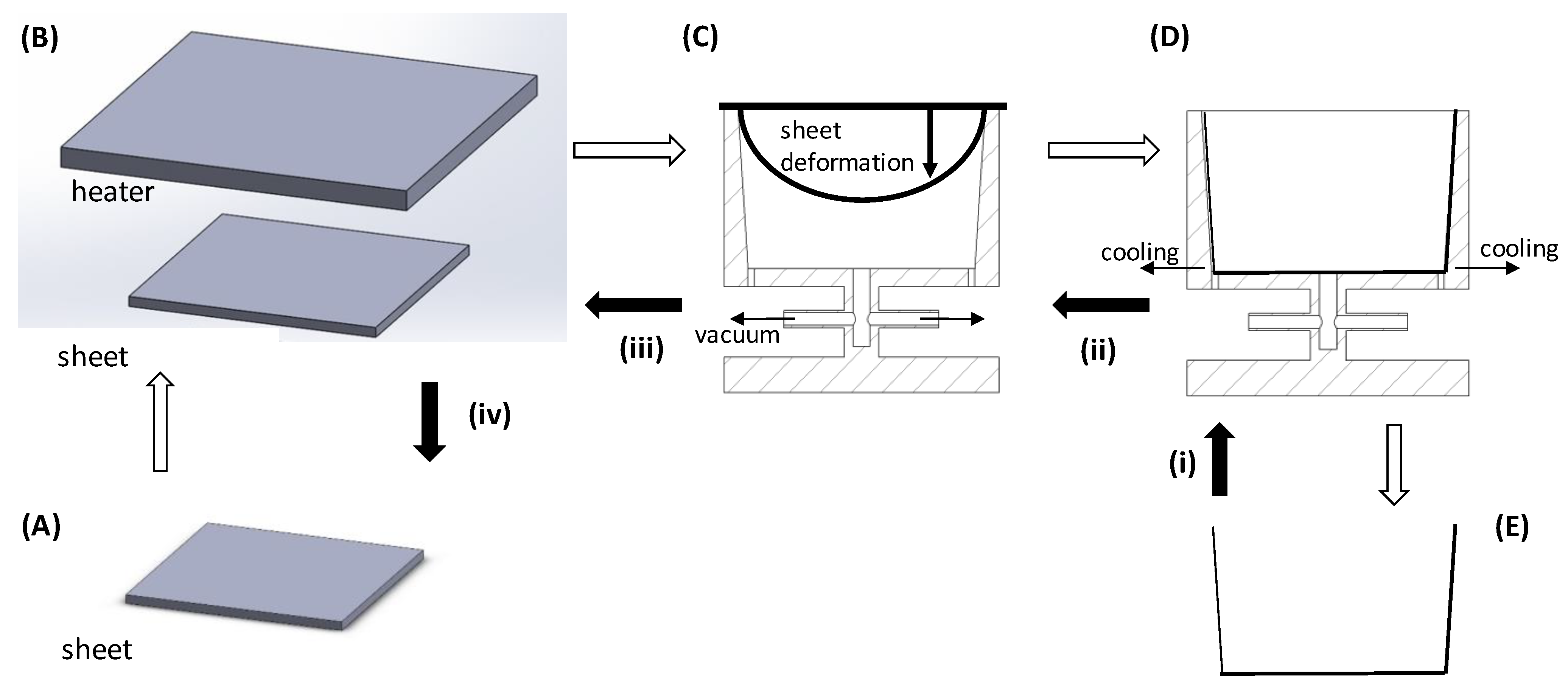
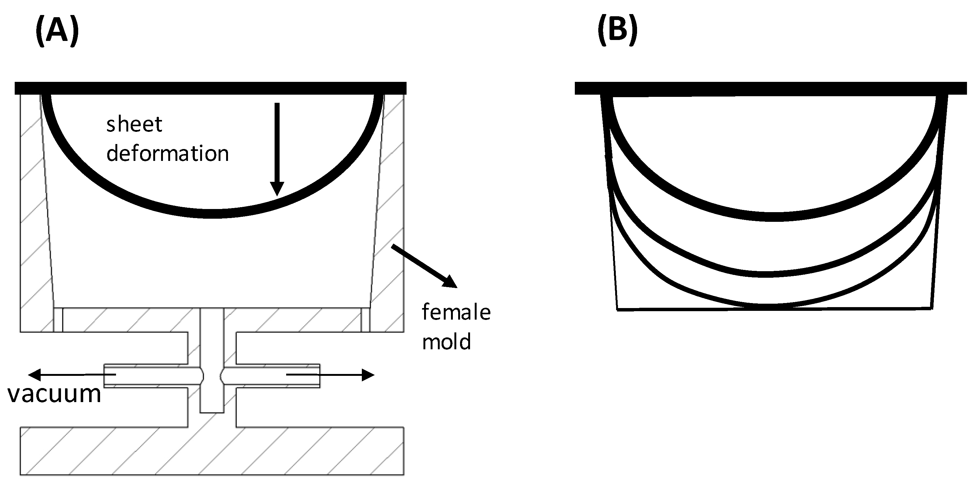
2.1. The Process

Figure 1 illustrates schematically the thermoforming phases and the optimization sequence. The phase order is indicated by open arrows and consist basically of: (A) producing a plastic sheet, typically by extrusion; (B) heating the sheet until it can be deformed without breaking; (C) shaping the sheet against the contours of a mold by applying a pressure difference on both sides, either by vacuum or pressurized air; (D) cooling the product obtained to make it possible to remove it from the mold and (E) remove the part from the mold. Each one of these phases has particular characteristics that must be considered when optimizing the process, either in terms of what concerns the operating conditions (e.g., heating and cooling times, air pressure and oven temperatures) and/or design parameters (e.g., sheet thicknesses, heater location, heating methods and mold geometry) [16,17].

Figure 2 shows schematically how the shaping process evolves. The heated sheet is forced to deform by the action of a pressure differential between both sides of the sheet. Initially, this deformation is uniformly distributed, but when it touches the cold mold surfaces the plastic material is frozen and only the remaining part of the sheet continues to deform. This implies that the last part of the sheet touching the mold will present the lowest thickness, since that the total volume of the sheet is conserved. This corresponds to the region of the lower corners in Figure 2B.

Therefore, the most important objective when producing a thermoformed part is to guarantee that its final thickness is as uniform as possible. This requirement is necessary in order to be possible to accomplish two main objectives, mainly in the shaping phase: to minimize the amount of material necessary and to maximize the mechanical behavior and/or other required characteristics.

To produce a part with uniform thickness, it is possible to act in different phases of the process. First, as shown in Figure 3, it is possible to produce sheets with different thicknesses at different regions of the part to be produced. Therefore, in the regions where more deformation occurs during the shaping phase, and, as a consequence, the thickness of the part will be smaller, it is possible to increase the thickness of the original sheet. Three situations are possible, as illustrated in Figure 3: (A) constant sheet thickness, (B) variable sheet thickness in one direction (x) and (C) variable sheet thickness in two directions (x and y). However, the processes used to produce the sheets are different, which must be taken into account in any optimization process since the costs can be very different as well. While (A) and (B) can be produced by extrusion, (C) must be produced by injection molding, given the specific and complicated geometry. While the sheet with constant thickness (A) can be produced in the usual way, using a flat die and a calender, to produce sheet (B) it is necessary to change the die and the calender rolls in order to induce different thicknesses.

Secondly, the sheet deformation during the shaping phase depends on the mechanical properties of the polymeric material used at the heating temperature. This temperature dependency makes it possible to obtain different sheet deformations in order to control the thickness distribution, that is, in the regions where more deformation is required, the temperature must be lower [11,18]. Figure 4 illustrates schematically the process of heating the plastic sheet. Several parameters can be considered: (i) the number of heaters, for example, for sheets with higher thickness two heaters can be used, one each side; (ii) the distance between the heaters bank and the sheet; (iii) the dimensions of each individual heater and (iv) temperature of each individual heater. This approach is illustrated in Figure 4, where a mesh of heaters (e.g., ceramic heaters) can be used, each one with the possibility of having different temperature distributions. In any case, it is fundamental to control the correct temperature in the entire sheet surface. In practice, and given the lower heat conductivity of plastics, a temperature gradient along the thickness of the sheet will arise. Furthermore, and if radiation heating is used, due to geometric reasons, the temperature at the center of the sheet will be higher than in its edge [19,20]. From the practical point of view and after the heating phase, the temperature of the entire sheet must be in the range of the forming temperatures. This temperature window is intrinsic to each polymer.

Third, a straightforward way of minimizing the difference of thicknesses in the part thermoformed is related to the process of shaping. For that purpose, several thermoforming variants can be used: female mold (as illustrated in Figure 2), male mold, plug assisted, bubble forming, bubble forming and plug assisted and other combinations of the above [21,22,23,24,25].

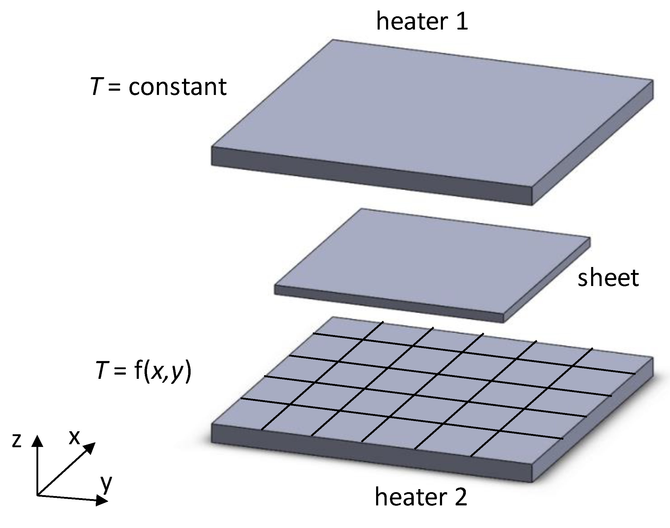
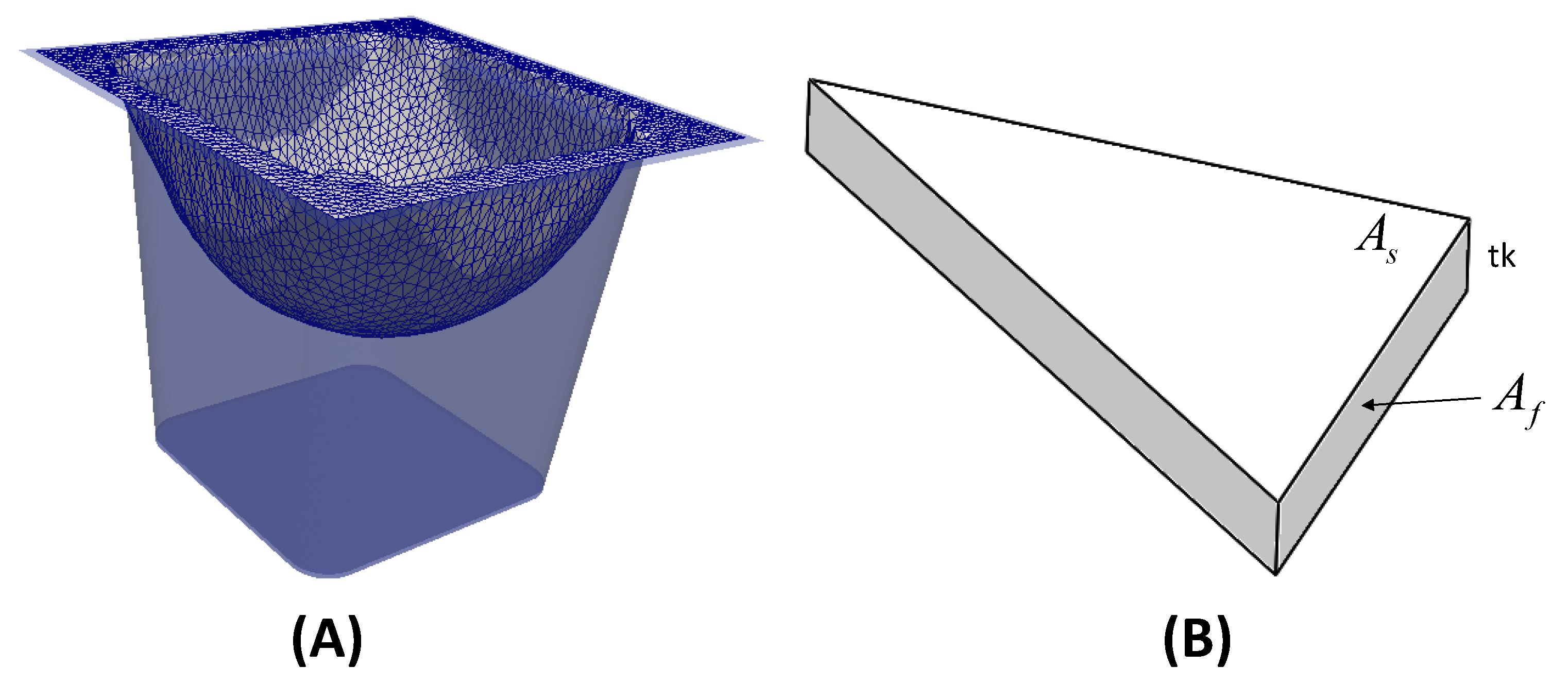
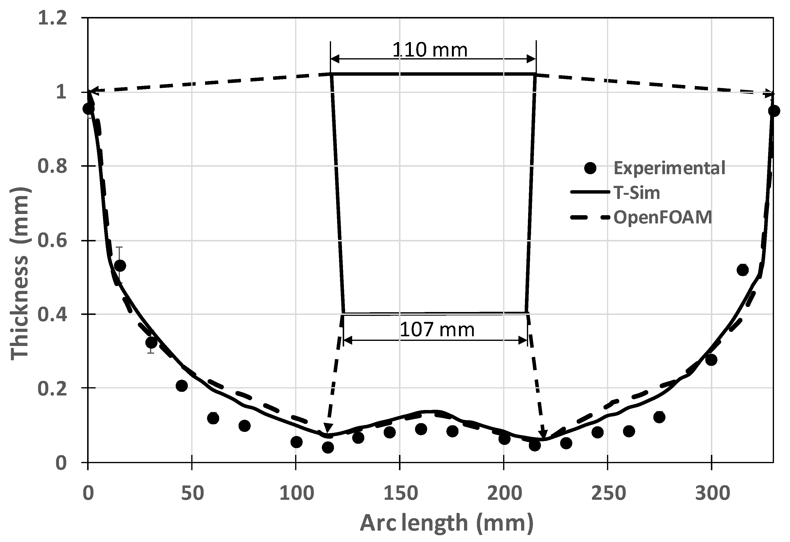
2.2. Numerical Modeling

During the inflation process, the polymer sheet deforms due to the pressure difference imposed on both sides. Additionally, due to the deformation process, internal stresses are generated, which will limit the deformation promoted by the pressure difference. If the balance from those two loads is not null the velocity of the sheet changes, that is, there is a non-null acceleration.

For the adopted numerical approach, the polymer sheet is discretized into different computational cells as illustrated in Figure 5A. Moreover, the sheet is assumed to be thin enough to allow resorting to a membrane formulation, thus it is discretized into planar triangular cells each one with thickness tk (Figure 5B).

Considering the conditions above, the conservation of linear momentum is given by:

$$\mathsf{\rho }\frac{{\partial }^2\mathit{u}}{\partial t^2}=\nabla ·\sigma +\mathsf{\rho }\mathit{g},$$

(1)

where $t$ is time, $\mathsf{\rho }$ is the density, $\mathit{u}$ is the displacement vector, $\sigma$ is the Cauchy stress tensor and $\mathit{g}$ is the gravitational acceleration vector. Following the classical Finite Volume Method approach, Equation (1) is integrated into the space in a computational cell with volume $\mathsf{\Omega }$ and surrounded by the surface $\mathsf{\Gamma }$, which, after applying the Gauss Divergence theorem results in:

$$\underset{\mathrm{Inertia}}{\underbrace{{{\displaystyle \int }}_{\mathsf{\Omega }}\mathsf{\rho }\frac{{\partial }^2\mathit{u}}{\partial t^2}d\mathsf{\Omega }}}=\underset{\mathrm{Surface} \mathrm{Forces} }{\underbrace{{{\displaystyle \oint }}_{\mathsf{\Gamma }}\mathit{n}\cdot \mathbf{\sigma }d\mathsf{\Gamma }}}+\underset{\mathrm{Body} \mathrm{Forces} }{\underbrace{{{\displaystyle \int }}_{\mathsf{\Omega }}\mathsf{\rho }\mathit{g}d\mathsf{\Omega }}},$$

(2)

which shows that the acceleration of the computational cell is affected by the surface and body forces. For the body forces, only the weight due to gravity is considered, which can be obtained by:

$${\mathit{F}}_{Body}=\mathsf{\rho }\mathit{g}{V}_c$$

(3)

where $V_c$ is the computational cell volume.

The surface forces are of two types, namely external and internal forces. Following the membrane formulation, the external forces are due to the pressure difference between the inner and outer surfaces and the internal forces result from the stress induced by the material deformation. Based on Equation (2), where, in each time step, the acceleration of each computational cell is an explicit function of the applied loads, the surface forces are the sum of the internal and external forces and can be calculated by the following equation:

$${\mathit{F}}_{Surface}={{\displaystyle \oint }}_{\mathsf{\Gamma }}\mathit{n}\cdot \mathbf{\sigma }d\mathsf{\Gamma }={{\displaystyle \int }}_{{\mathrm{A}}_S}p{\mathit{n}}_{s}d{\mathrm{A}}_S+{{\displaystyle \int }}_{{\mathrm{A}}_f}{\mathit{n}}_f\cdot \tau d{\mathrm{A}}_f={\mathit{F}}_{pressure}+{\mathit{F}}_{internal}$$

(4)

where $p$ is the imposed pressure difference, $\tau$ the internal stress vector, ${\mathrm{A}}_S$ the cell surface area (see Figure 5), with normal vector ${\mathit{n}}_s$ and ${\mathrm{A}}_f$ the cross-sectional cell area, with normal vector ${\mathit{n}}_f$. The internal forces are calculated at each cell cross section along the thickness. Due to the quick deformation process that takes place in thermoforming, which has been shown to be mostly elastic since the original shape of the sheet if the plastic part is heated [26], for this problem, the relation between the internal stresses was assumed to be based on the elasticity theory:

$$\tau =ℂ:\mathbf{ϵ}$$

(5)

where $ℂ$ is the stiffness fourth-order constitutive tensor and $\mathbf{ϵ}$ the strain tensor. In this, $\tau$ and $\mathbf{ϵ}$ must be work conjugate pairs of stresses and strains respectively. Considering the membrane formulation, the elastic solid undergoes through large displacements, large rotations and large strains and non-linearity cannot be neglected, the proper work conjugate pair of stresses and strains are the Second Piola–Kirchhoff stress tensor, for $\tau$ and the Green–Lagrange strain tensor, for $\mathbf{ϵ}$, which is given by:

$$\mathbf{ϵ}=\frac{1}{2}\left({\mathit{F}}^{\mathit{T}}·\mathit{F}-\mathit{I}\right)$$

(6)

In Equation (6), $\mathit{F}$ is the deformation gradient tensor, given by the derivative of each component of the deformed position $\mathit{x}$ vector with respect to each component of the reference position $\mathit{X}$ vector, and $\mathit{I}$ is the unit tensor. This formulation is equivalent to the hyperelastic Saint Venant–Kirchhoff model [27].

On the implemented explicit numerical procedure, at each time step all the loads are calculated with Equations (3)–(7) and the acceleration of each cell is given by Equation (2). This allows one to calculate the new cell position and advance to the next time step.

On all the numerical studies performed in this work an elastic modulus of 10 MPa was employed, which is representative of HIPS at the usually employed processing temperature of 140 °C [28]. Moreover, the material was assumed to be incompressible, thus, a Poisson’s ratio of 0.5 was considered.

2.3. Experimental Assessment

The modeling computational results were assessed using the circular cup illustrated in Figure 6 [29]. The experimental work was performed on a modified Illig thermoforming machine that allows individual monitoring and control of the main thermoforming variables. The heater bank included 110 Elstein 125 W ceramic radiators (each 120 × 60 mm). Square portions of the sheet were cut and manually clamped (fixed) on all four sides, in such a way that the material was not allowed to slide into the mold cavity. Once the heating stage is completed and a uniform sheet temperature of 150 °C is reached, the frame (holding the sheet) moves toward the forming station. The lower mold section moves vertically, clamping the sheet circularly. The parts were vacuum-formed at 0.7 bar. After forming and cooling, the cups were extracted, cut into four equal portions along a line passing by the center of the base midpoint and their thicknesses along that line and circumferentially were measured with a caliper (precision of 0.01 mm). At least five cups were produced for each set of variables. The results are generally presented along the arc length but correspond to averages in the circumferential direction. The material used in the sheets is a mixture of 50% Polystyrene (PS Laquerene 1540) with 50% Impact Polystyrene (HIPS Laquerene 7240), both produced by Elf-Atochem.

The theoretical results were computed using a commercial software T-SIM using a K-BKZ viscoelastic model whose material properties are described in [29] and by using the OpenFOAM considering the hyperelastic Saint Venant–Kirchhoff model for the material. As can be seen, the computational results show a good agreement with the experimental measurements, the behavior of both theoretical models being very similar. In fact, regarding the simulation of the thickness distribution in thermoforming, it is possible to find, throughout the literature, several works that use hyperplastic models (e.g., Ghobadnam [30], Bernard et al. [31], Oueslati et al. [32], Jeet et al. [33]) and viscoelastic models (e.g., Cha et al. [34], Atami et al. [28]). Although researchers are increasingly turning to viscoelastic models for thermoforming applications, according to O’Connor et al. [35], there is little agreement on the best model to use for any given polymer material.

Furthermore, the use of hyperelastic models is based on the experience reported by Schmidt and Carley [26] and Rosenzweig et al. [36]. They described the “plastic memory”, where blown bubbles returned completely to their original flat sheet form, either by suddenly releasing the forming pressure or by annealing spheroidal bubbles at a proper temperature. The observation of complete recovery has led the authors to conclude that elastic-like behavior can be ascribed to the processes of blowing soft plastic sheets.

Therefore, and considering that the main objective of this work is to evaluate the optimization process and not to predict more accurately the thickness distribution, and for computation time reasons, a hyperelastic model was chosen to predict the plastic sheet behavior during the forming process.

3. Multi-Objective Optimization

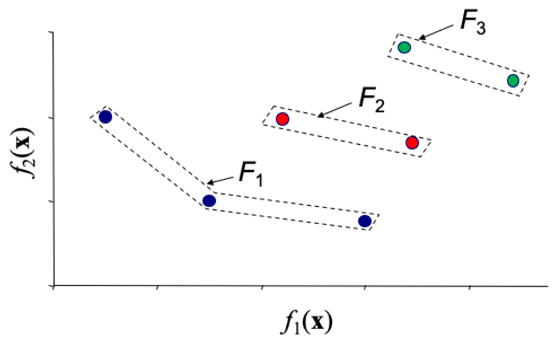
3.1. Multi-Objective Evolutionary Algorithms

In a Multi-Objective Optimization Problem (MOP), the goal is to minimize all objectives simultaneously, that is, to find feasible solutions where every objective function is minimized. A multi-objective optimization problem with $m$ objectives and $n$ decision variables can be formulated as follows:

$$\begin{array}{cc}\underset{\mathit{x}\in \mathsf{\Omega }}{\min }& \mathit{f}\left(\mathit{x}\right)\equiv (f_1\left(\mathit{x}\right),\dots ,f_m\left(\mathit{x}\right))\\ \mathrm{subject} \mathrm{to}& g_i\left(\mathit{x}\right)\le 0,i\in \left\{1,\dots ,p\right\}\\ & h_j\left(\mathit{x}\right)=0, j\in \left\{1,\dots ,q\right\}\\ & \mathit{l}\le \mathit{x}\le \mathit{u}\end{array}$$

(7)

where $\mathit{x}$ is the decision vector, i.e., $\mathit{x}\in \mathsf{\Omega }\subseteq R^n$, $\mathit{f}$ is the objective vector of $m$ objective functions, that is, $\mathit{f}\in \mathsf{\Omega }\subseteq R^m$, $g_i$ are $p$ inequality constraint functions and $h_j$ are $q$ equality constraint functions and $\mathit{l}$ and $\mathit{u}$ are the vectors of the lower and upper bounds on decision variables, respectively.

Solutions are compared in terms of Pareto dominance, that is, a solution $\mathit{x}$ is said to dominate a solution $\mathit{y}$ ($\mathit{x}\prec \mathit{y})$, if and only if $f_i\left(\mathit{x}\right)\le f_i\left(\mathit{y}\right)$, for all $i\in \left\{1,\dots ,m\right\}$ and $f_j\left(\mathit{x}\right)<f_j\left(\mathit{y}\right)$ for at least one $j\in \left\{1,\dots ,m\right\}$. If all objectives do not conflict with each other, there exists a unique solution that minimizes all the objectives. In general, there are multiple conflicting objectives giving rise to a set of optimal solutions—the Pareto optimal set, instead of a single optimal solution. A feasible solution, ${\mathit{x}}^{*}$ is Pareto optimal if and only if there is no other solution $\mathit{y}\in \mathsf{\Omega }, \mathit{y}\ne {\mathit{x}}^{*}$, that $\mathit{y}\prec {\mathit{x}}^{*}$. These solutions are incomparable to each other since none of these solutions can be said to be better than others.

In order to facilitate the decision-making process, an a posteriori method in which the search for an approximation (as close and diverse as possible) to the Pareto optimal set is performed before the decision-making process. Thus, the decision-maker can select the most suitable solution from this set according to their preferences. The Pareto optimal set provides valuable information with respect to the trade-offs between alternatives.

There is a large variety of approaches to solving MOPs. The designated classical (or traditional methods) are known as scalarization methods in which the MOP is reformulated and solved as a single objective optimization problem [37]. However, usually, scalarization functions involve several parameters that can be difficult to define in order to obtain different approximations to the Pareto optimal solutions. Other approaches are based on Evolutionary Algorithms (EAs). EAs are meta-heuristics that mimic the process of evolution of a population of individuals over generations. The fittest individuals to the environment will survive over time and therefore will be likely to reproduce. The offspring are generated by genetic operators, such as crossover and mutation and inherit the parent characteristics. Basically, in EAs, a population of individuals representing a candidate solution to the problem evolves using two mechanisms: Selection and Variation. The quality of each individual is measured using a fitness function that, in optimization problems, is related to the objective or objectives functions for single or multi-objective optimization problems, respectively. The selection mechanism guarantees that the best individuals have a higher probability of being selected for generating offspring. The variation mechanism provides the generation of new individuals by application of genetic operators.

Multi-Objective Evolutionary Algorithms (MOEAs) are EAs for solving MOPs. There are advantages to using this type of algorithms. They work with a population of candidate solutions, which makes it possible to approximate the entire Pareto optimal set in a single run. The performance of any MOEA is strongly related to the efficacy of its Selection mechanism that guides the search in the objective space, balancing convergence and diversity and also the variation mechanism that is responsible for the generation of offspring. A common approach to simulating natural selection in MOEAs consists of assigning fitness values to individuals in the population according to its quality for the MOP being solved. In terms of the type of fitness function used, MOEAs can be classified into three different types: dominance-, scalarizing- and indicator-based algorithms.

Dominance-based approaches calculate an individual’s fitness on the basis of the Pareto dominance relation [38] or according to different criteria [39]. Scalarizing-based approaches [40] incorporate traditional mathematical techniques based on the aggregation of multiple objectives into a single parameterized function. Indicator-based approaches use performance indicators for fitness assignment; pairs of individuals are compared using some quality measure such as the hypervolume indicator [41,42]. The fitness value reflects the loss in quality if a given solution is removed [42,43].

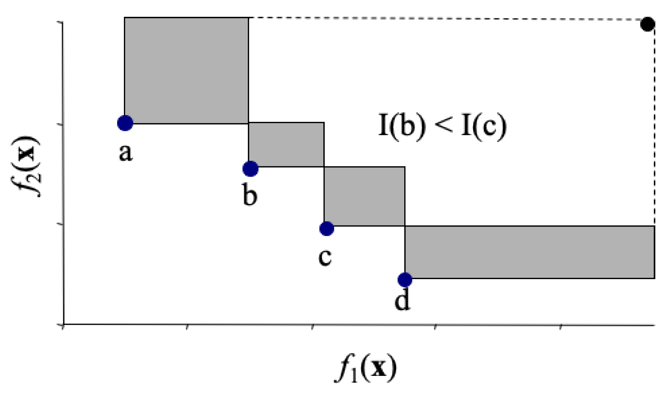
3.2. SMS-EMOA

The multi-objective evolutionary optimization algorithm used in this work is based on the SMS-EMOA [32] and implemented in MATLAB. The outline of the SMS-EMO is given by Algorithm 1.

Algorithm 1 SMS-EMOA

$P_0\leftarrow initialize()$     % Initialize population at random with $\mu$ individuals

$k\leftarrow 0$

Repeat

$q_{k+1}\leftarrow generate\left(P_k\right)$   % generate offspring by genetic operators

$P_{k+1}\leftarrow selection\left(P_k{{\displaystyle \cup }}^{ }\left\{q_{k+1}\right\}\right)$   % select $\mu$ best individuals

$k\leftarrow k+1$

Repeat until the stopping criterion is fulfilled

The search starts from an initial population of $\mu$ individuals randomly generated satisfying the boundary constraints of the decision variables. In each generation, one parent is selected at random from the population and a single offspring is produced by application of a variation procedure. In this procedure, a Gaussian mutation with covariance matrix adaptation [44] is applied to the parent to produce a single offspring. Next, a deterministic selection procedure selects the $\mu$ best individuals to the next generation. The selection involves the non-dominated ranking of the population and the computation of the hypervolume contribution of each individual of the population.

The non-dominated sorting procedure is illustrated in Figure 7. First, the $P_k{{\displaystyle \cup }}^{ }\left\{q_{k+1}\right\}$ individuals are ranked according to a non-dominated sorting procedure defining $f$ fronts of sets of non-dominated individuals [28]. A rank is assigned to each front representing its level of domination. All solutions belonging to each front are incomparable. The first front $F_1$ contains the non-dominated solutions in $P_k{{\displaystyle \cup }}^{ }\left\{q_{k+1}\right\}$. The second front $F_2$ contains all non-dominated solutions in $P_k{{\displaystyle \cup }}^{ }\left\{q_{k+1}\right\}\backslash F_1$. This procedure is repeated until all solutions in $P_k{{\displaystyle \cup }}^{ }\left\{q_{k+1}\right\}$ are included in a front. Any solution in front $F_{i+1}$ is dominated by at least one solution of front $F_i$ for $i\ge 1$.

Afterward, the hypervolume contribution [39] of each individual in the last front $P_k{{\displaystyle \cup }}^{ }\left\{q_{k+1}\right\}$ is computed. Hypervolume definition guarantees that any non-dominated solution will not be replaced by a dominated solution since non-dominated solutions will have a higher hypervolume contribution than dominated ones. Hypervolume allows one to obtain a well-distributed set of solutions in the objective space as well as to guide the search toward the Pareto optimal front.

The hypervolume contribution computation is straightforward for problems with two objectives [41]. The approximations to the ideal vector ($z_i^{*})$ and the nadir vector ($z_i^{nad})$ computed in the current population are used to normalize objectives functions to the same order of magnitude in the interval [0,1]. The normalized objective function $f_i^{norm}$ for the $i$-th objective function is computed by:

$$f_i^{norm}=\frac{f_i-z_i^{*}}{z_i^{nad}-z_i^{*}}.$$

(8)

The solutions of the worst-ranked non-dominated front are sorted in ascending order according to the values of the first normalized objective function. A sequence that is additionally sorted in descending order is obtained since the solutions are mutually non-dominated. Then, the hypervolume contributions of the solutions can be obtained by computing the rectangle area as illustrated in Figure 8. Given a sorted front with $r$ solutions $F=\left\{s_1,s_2\dots ,s_r\right\}$, the hypervolume contribution of solution $s_i$ ($I\left(s_i\right)$) is computed by [39]:

$$I\left(s_i\right)=\left(f_1\left(s_{i+1}\right)-f_1\left(s_i\right))\times (f_2\left(s_{i-1}\right)-f_2\left(s_i\right)\right)$$

(9)

where $i=2,\dots ,r-1$.

In Figure 8, it can be seen that the hypervolume contribution of solution b is inferior to c, as the area covered by b is smaller, which implies that this solution will not be selected in the next generation.

The $\mu$ best individuals in terms of the domination ranking are selected to be the progenitors of the next generation. On the last front, the individual with the worst hypervolume contribution is discarded. This process is repeated until the stopping criterion is fulfilled.

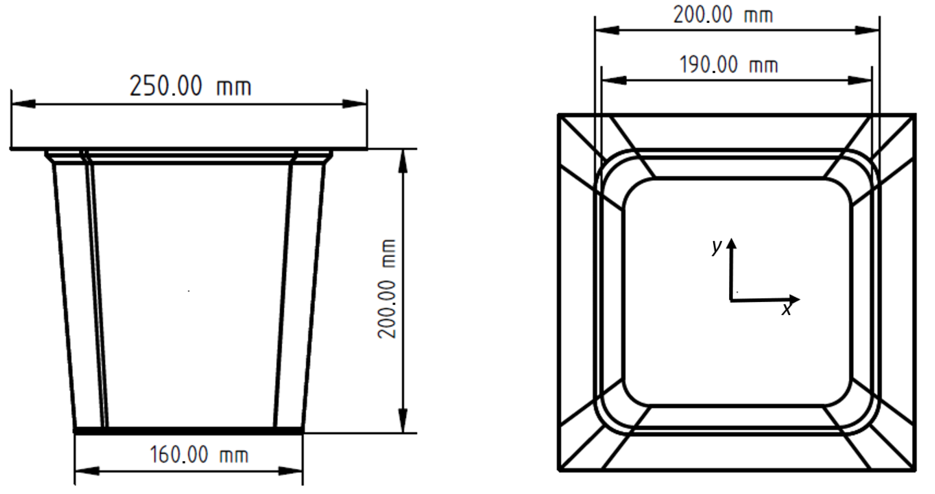
4. Case Study

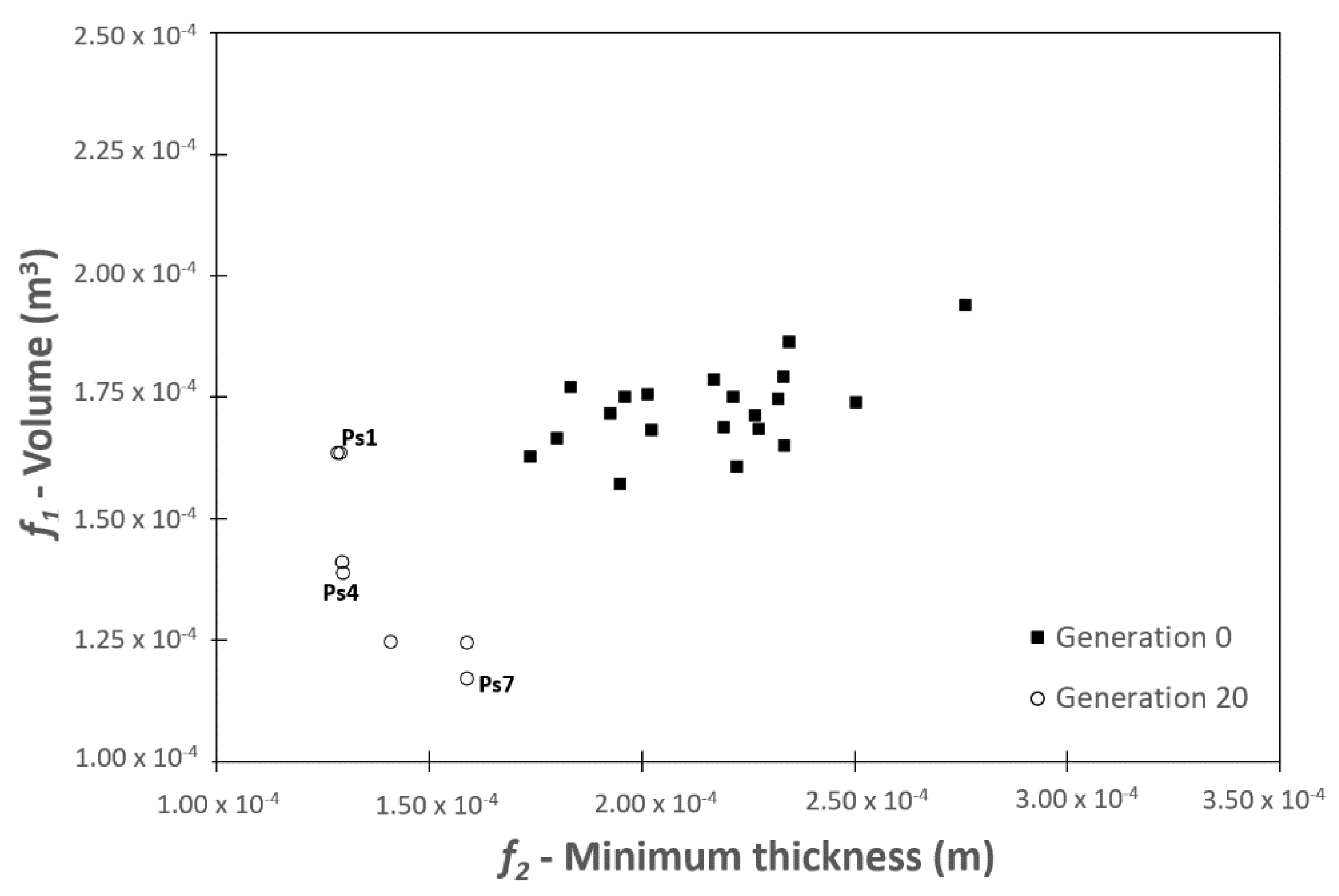
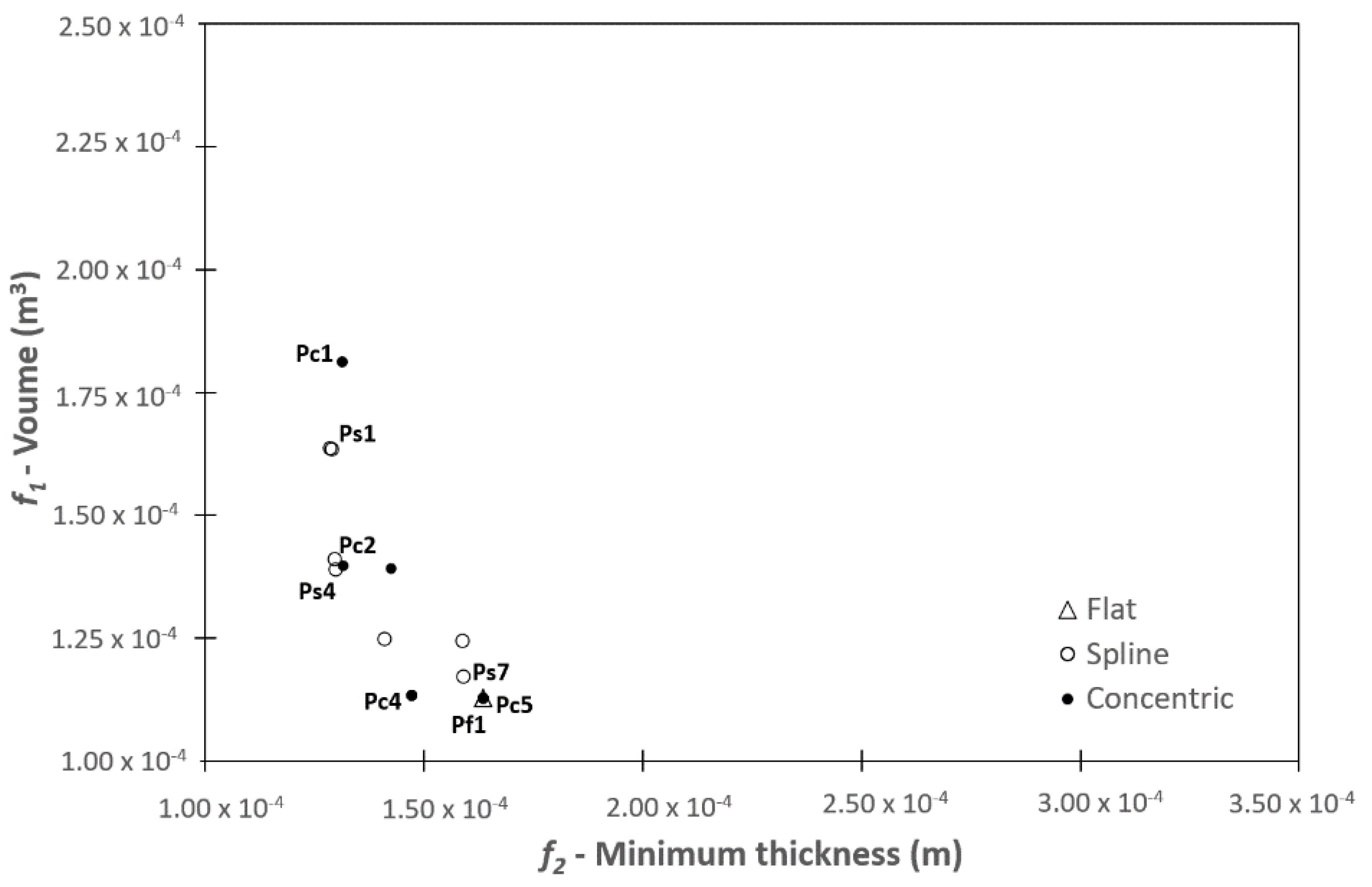
4.1. The Optimization Problem to Solve

In the present study, the cup illustrated in Figure 9 was thermoformed with constant temperature, a female mold and three types of sheets (as shown in Figure 3): constant thickness, linear spline variation and concentric spline variation. The aim was to determine the sheet thickness profile in order to: (i) minimize the initial sheet volume, as it implies less material use (f₁); (ii) minimize the minimum thickness found in the cells of the mesh used in the modeling calculations without hindering its mechanical behavior, as it is related with the capacity of the polymer sheet deformability, representing indirectly a measure of the thickness heterogeneity (f₂); and (iii) minimize the thickness heterogeneity, that is, the difference between the thickness of the part and a reference thickness, as defined by Equation (10) (f₃).

$$f_3=\frac{1}{M}{\displaystyle \sum }_{i=1}^M\frac{\left|t_0-t_i\right|}{t_0}$$

(10)

where M is the number of points located in a line defining the center of the cup in direction x, t₀ is a reference thickness defined by the user and t_i are the thicknesses of the M points.

This is a bound constrained multi-objective optimization problem with the following decision variables and objectives limitations (dimensions in meters):

$$\begin{array}{c}2.0\times {10}^{-3}\le x_i\le 4.0\times {10}^{-3}\\ Minimum thickness\ge 1.0\times {10}^{-4}\end{array}$$

(11)

where x_i is the sheet thickness of the constant thickness along the x direction. The thickness along the x direction is then imposed using a spline variation based on the 10 control points (see Figure 3), or the thickness of the five control points determining the concentric thickness variation, from the center to the border of the circle represented in Figure 3C. First, three bi-objective problems were considered (Cases 1 to 3), one for each case of sheet thickness variation and taking into account objectives f₁ and f₂, with the aim of showing the effectiveness of the methodology in solving this problem. Then, two bi-objective problems using objectives f₁ and f₃ were considered (Cases 4 and 5, respectively with spline and concentric variations), the aim being to approach the solutions to a more realistic industrial situation.

The multi-objective evolutionary algorithm used in this work is based on the SMS-EMOA. Considering the characteristics of the multi-objective optimization problem being solved, different configurations and search mechanisms can be adopted for SMS-EMOA. Thus, as described in Section 3.2, Gaussian mutation with covariance matrix adaptation was selected as the variation procedure, since the problem being solved comprises continuous variables. simultaneously, the hypervolume metric was chosen to provide well-distributed alternative solutions in the objective space. The configuration, including the parameter values of the algorithm, takes into account the considerable computational effort required to compute the objective function values. The population size was set to 20 individuals. The selection was carried out using a uniform distribution and variation was performed by the CMA evolution strategy operator [8], which is designed to work with real number representations. The maximum number of generations was set to 20.

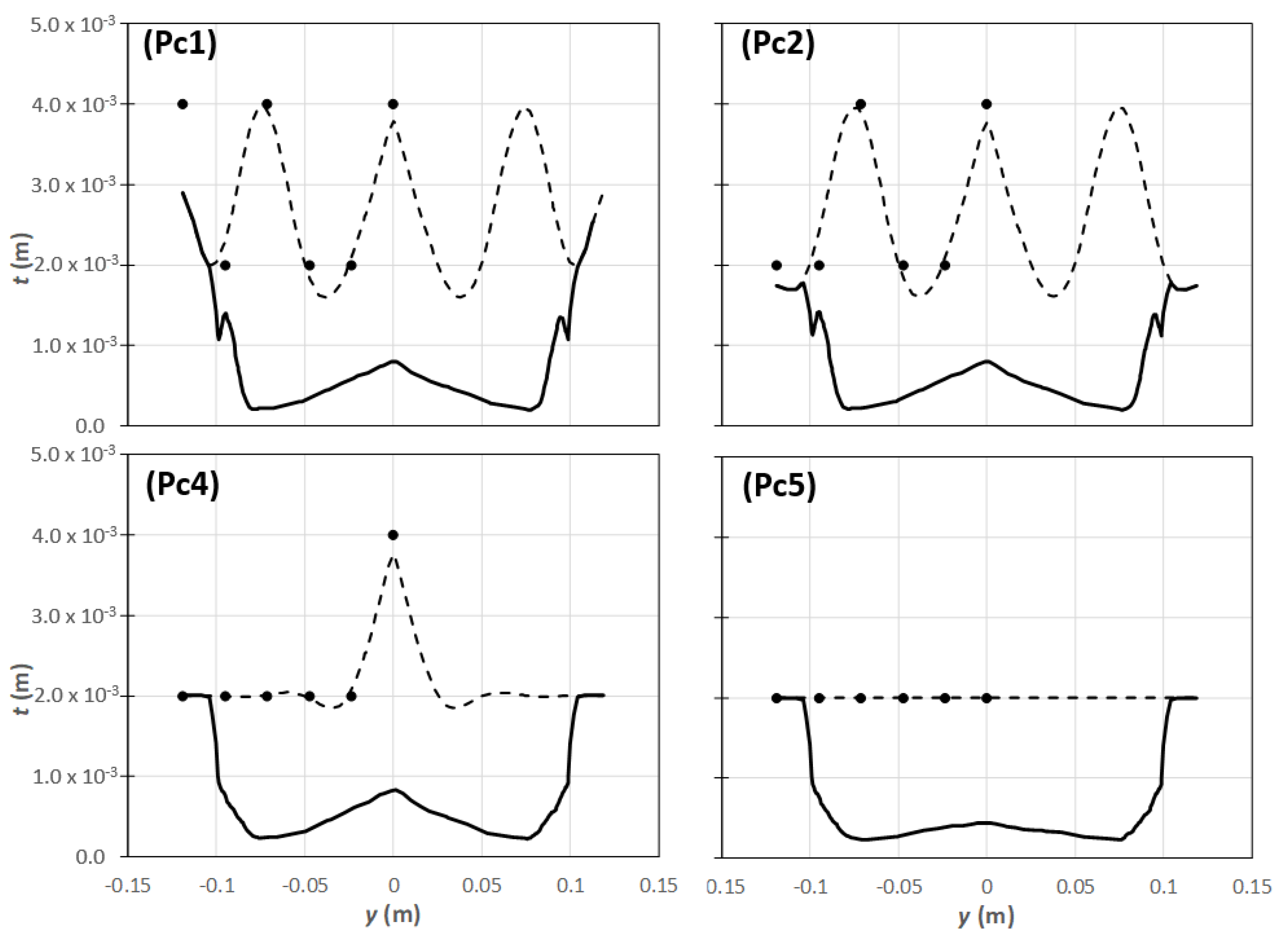
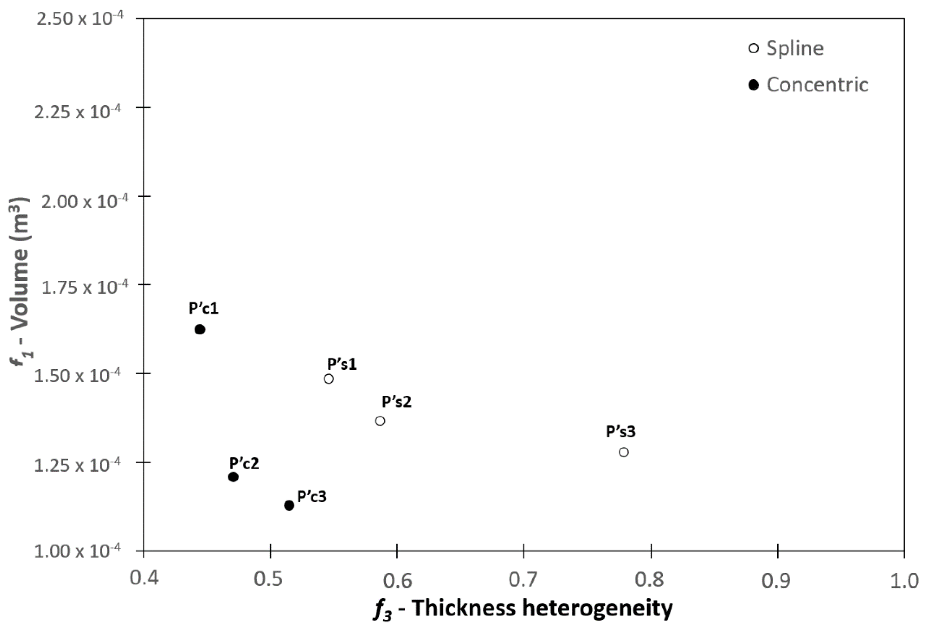
4.2. Results and Discussion

For Case 1, the sheet with constant thickness, both objectives (volume and thermoformed part minimum thickness) are in harmony, which means that the solutions of all generations are located in a line and the single optimal solution is the one more near the minimum of these two objectives. The same does not occur for the other two cases.

Figure 10 shows the random initial population and the non-dominated solutions of the last generation for optimization Case 2, which comprises seven solutions. In this case, the sheet thickness is a spline generated from the 10 decision variables represented by black dots in the graphs, provided in Figure 11. It is clear that there is improvement along the 20 generations. The Pareto optimal front of the last generation presents some gaps between the solutions due to the thermoforming problem characteristics, as the location of the 10 points used to generate the sheet spline thickness are fixed and equally spaced along the x axis, which limits the search space.

The sheet and final part thickness profiles of solutions Ps1, Ps4 and Ps7 are illustrated in Figure 11. As can be seen in the graphs, the thickness profiles perpendicular to the spline (Figure 11-left), when moving from solutions Ps1 to Ps7 the final part profile, are more uniform. From the point of view of the Decision-Maker, this seems to indicate that Ps7 is the best solution for practical purposes. This evidences the great advantage of performing this type of multi-objective optimization. Not only does the algorithm converge to better solutions, but it can also provide the Decision-Maker a set of solutions from which he can choose the best one to be applied in the real thermoforming practice, in this case, solution Ps7. Another characteristic of the solutions shown is that for x equal to zero (Figure 11-left) the sheet spline thickness is the same in all cases (t ≈ 2.0 × 10⁻³ m), which produces identical part profiles in the transversal direction, as illustrated by the graphs of Figure 11-right.

Figure 12 shows the Pareto optimal solutions for all the cases studied. As can be seen, in Case 3 (concentric spline), the optimization converges to five non-dominated solutions, identified by black dots. The final part thickness profile of four solutions for this case, Pc1, Pc2, Pc4 and Pc5 are represented in Figure 13 (solution Pc3 was not represented due to its similarity with solution Pc2). The black dots identify the location of the points used to generate the symmetrical concentric spline represented by a dashed line, the decision variables. Again, from solution Pc1 to solution Pc5, the profile obtained is more uniform, as in Case 2. Also, it is important to note that, in this case, the part thickness profile is the same in all directions, as the sheet thickness presents an axisymmetric distribution.

Figure 14 shows the part thickness profile of the unique solution found for Case 1, Pf1. As can be seen, the profile obtained is very similar to that of solutions Ps7 and Pc5 of the previous cases studied. This confirms that the optimization strategy is working and identify solutions with physical meaning, since different starting points, corresponding to diverse initial sheet thickness profiles, led to identical solutions when those solutions are located in the same region of the search space, as can be seen in Figure 12.

Finally, Figure 15 shows the non-dominated solutions of the 20th generation for Cases 4 and 5, considering spline and concentric sheet thickness variation and t₀ equal to 0.5 mm. As previously, the gaps between the solutions are due to the problem constraints related to a limited search space. It is clear that, as expected, the concentric variation produces much better results concerning the uniformity of the thickness. Solutions P’s3 and P’c3 are the same as those obtained previously, that is, solutions Ps7 and Pc5. However, the solutions found depend strongly on the value chosen for t₀. A practical alternative consists of finding the desired thickness profile for the final part through a mechanical analysis, for example, as suggested in the scheme of Figure 1.

Also, it is important to note that technically and economically it is difficult to produce concentric initial sheet variations, as it implies high costs, mainly when the parts are to be produced in big quantities, as is commonly the case.

5. Conclusions

Faced with the complexity of the real optimization problem in the field of plastics thermoforming described in this paper, the applicability of a multi-objective optimization strategy was proposed to deal with the process forming phase. The aim was to determine the better sheet thickness distribution that allows the production of parts with the least amount of material while assuring the appropriate characteristics of the final part. A reduction of circa 30% in the volume of the material used can be obtained when comparing the solutions of the initial population and the ones in the Pareto front.

The main scientific contribution of this work is to add a new approach to control the thickness distribution of thermoformed parts, in addition to the variations of technique and differential heating previously mentioned. Since the final thickness of the parts depends on the initial thickness of the sheet, several solutions are proposed for adjusting the initial thickness of the sheet in order to achieve the most favorable thickness.

The results obtained showed that the methodology proposed was able to capture the singular features of the process allowing us to conclude that the strategy proposed might be successfully applied in the optimization of the various steps of plastics thermoforming. This work constitutes a further step to support design approaches associated with this important plastics processing technology.

References

- Yang, C.; Hung, S.-W. Modeling and Optimization of a Plastic Thermoforming Process. J. Reinf. Plast. Compos. 2004, 23, 109–121. [Google Scholar] [CrossRef]
- Chang, Y.-Z.; Wen, T.-T.; Liu, S.-J. Derivation of optimal processing parameters of polypropylene foam thermoforming by an artificial neural network. Polym. Eng. Sci. 2004, 45, 375–384. [Google Scholar] [CrossRef]
- Leite, W.D.O.; Rubio, J.C.C.; Cabrera, F.M.; Carrasco, A.; Hanafi, I. Vacuum Thermoforming Process: An Approach to Modeling and Optimization Using Artificial Neural Networks. Polymers 2018, 10, 143. [Google Scholar] [CrossRef] [PubMed] [Green Version]
- Leite, W.; Rubio, J.; Mata, F.; Hanafi, I.; Carrasco, A. Dimensional and Geometrical Errors in Vacuum Thermoforming Prod-ucts: An Approach to Modeling and Optimization by Multiple Response Optimization. Meas. Sci. Rev. 2018, 18, 113–122. [Google Scholar] [CrossRef] [Green Version]
- Sasimowski, E. The use of utility function for optimization of thermoforming. Polimery 2018, 63, 807–814. [Google Scholar] [CrossRef]
- Wang, C.-H.; Nied, H.F. Temperature Optimization for Improved Thickness Control in Thermoforming. J. Mater. Process. Manuf. Sci. 1999, 8, 113–126. [Google Scholar] [CrossRef]
- Bordival, M.; Andrieu, S.; Schmidt, F.; Maoult, Y.L.; Monteix, S. Optimization of Infrared Heating System for the Ther-Moforming Process. In Proceedings of the ESAFORM 2005-8th ESAFORM Conference on Material Forming, Cluj-Napoca, Romania, 27–29 April 2005; hal-01788422. pp. 925–928. [Google Scholar]
- Chy, M.M.; Boulet, B. A Conjugate Gradient Method for the Solution of the Inverse Heating Problem in Thermoforming. In Proceedings of the IEEE Industry Applications Society Annual Meeting, Houston, TX, USA, 3–7 October 2010; pp. 1–8. [Google Scholar]
- Chy, M.M.; Boulet, B.; Haidar, A. A Model Predictive Controller of Plastic Sheet Temperature for a Thermoforming Process. In Proceedings of the 2011 American Control Conference, San Francisco, CA, USA, 29 June–1 July 2011; pp. 4410–4415. [Google Scholar]
- Li, Z.; Heo, K.; Seol, S. Time-dependent Optimal Heater Control in Thermoforming Preheating Using Dual Optimization Steps. Int. J. Precis. Eng. Manuf. 2008, 9, 51–56. [Google Scholar]
- Li, Z.-Z.; Ma, G.; Xuan, D.-J.; Seol, S.-Y.; Shen, Y.-D. A study on control of heater power and heating time for thermoforming. Int. J. Precis. Eng. Manuf. 2010, 11, 873–878. [Google Scholar] [CrossRef]
- Erchiqui, F.; Nahas, N.; Nourelfath, M.; Souli, M. Metaheuristic algorithms for optimisation of infrared heating in thermoforming process. Int. J. Metaheuristics 2011, 1, 199–221. [Google Scholar] [CrossRef]
- Bachir Cherif, K.; Rebaine, D.; Erchiqui, F.; Fofana, I. Metaheuristics as a Solving Approach for the Infrared Heating in the Thermoforming Process; GERAD HEC, GERAD-G-2015-139; GERAD: Montreal, QC, Canada, 2015. [Google Scholar]
- Cherif, K.B.; Rebaine, D.; Erchiqui, F.; Fofana, I.; Nahas, N. Numerically Optimizing the Distribution of the Infrared Radiative Energy on a Surface of a Thermoplastic Sheet Surface. J. Heat Transf. 2018, 140, 102101. [Google Scholar] [CrossRef]
- Erchiqui, F. Application of genetic and simulated annealing algorithms for optimization of infrared heating stage in ther-moforming process. Appl. Therm. Eng. 2018, 128, 1263–1272. [Google Scholar] [CrossRef]
- Throne, J.L. Technology of Thermoforming; Hanser Publishers: Munich, Germany, 1966. [Google Scholar]
- DiRaddo, R.W.; Meddad, A. Sensitivity of operating conditions and material properties for thermoforming process. Plast. Rubber Compos. 2000, 29, 163–167. [Google Scholar] [CrossRef]
- Duarte, F.M.; Covas, J. On the Use of the Heating Stage to Control the Thickness Distribution in Thermoformed Parts. Int. Polym. Process. 2004, 19, 186–198. [Google Scholar] [CrossRef]
- Duarte, F.; Covas, J.A. IR sheet heating in roll fed thermoforming: Part 1-Solving direct and inverse heating problems. Plast. Rubber Compos. 2002, 31, 307–317. [Google Scholar] [CrossRef]
- Schmidt, F.M.; Le Maoult, Y.; Monteix, S. Modelling of infrared heating of thermoplastic sheet used in thermoforming process. J. Mater. Process. Technol. 2003, 143, 225–231. [Google Scholar] [CrossRef]
- McCool, R.; Martin, P.J. The role of process parameters in determining wall thickness distribution in plug-assisted thermoforming. Polym. Eng. Sci. 2010, 50, 1923–1934. [Google Scholar] [CrossRef]
- Marathe, D.; Rokade, D.; Busher, A.L.; Jadhav, K.; Mahajan, S.; Ahmad, Z.; Gupta, S.; Kulkarni, S.; Juvekar, V.; Lele, A. Effect of Plug Temperature on the Strain and Thickness Distribution of Components Made by Plug Assist Thermoforming. Int. Polym. Process. 2016, 31, 166–178. [Google Scholar] [CrossRef]
- Martin, P.; Duncan, P. The role of plug design in determining wall thickness distribution in thermoforming. Polym. Eng. Sci. 2007, 47, 804–813. [Google Scholar] [CrossRef]
- Sasimowski, E. A pressure-bubble vacuum forming process for polystyrene sheet. Adv. Sci. Technol. Res. J. 2017, 11, 180–186. [Google Scholar] [CrossRef]
- Ayadi, A.; Lacrampe, M.-F.; Krawczak, P. Bubble assisted vacuum thermoforming: Considerations to extend the use of in-situ stereo-DIC measurements to stretching of sagged thermoplastic sheets. Int. J. Mater. Form. 2019, 13, 59–76. [Google Scholar] [CrossRef]
- Schmidt, R.L.; Carley, J.F. Biaxial stretching of heat-softened plastic sheets using an inflation technique. Int. J. Eng. Sci. 1975, 13, 563–578. [Google Scholar] [CrossRef]
- Tuković, Ž.; Karač, A.; Cardiff, P.; Jasak, H.; Ivanković, A. OpenFOAM Finite Volume Solver for Fluid-Solid Interaction. Trans. FAMENA 2018, 42, 1–31. [Google Scholar] [CrossRef]
- Atmani, O.; Abbès, F.; Li, Y.; Batkam, S.; Abbès, B. Experimental investigation and constitutive modelling of the deformation behaviour of high impact polystyrene for plug-assisted thermoforming. Mech. Ind. 2020, 21, 607. [Google Scholar] [CrossRef]
- Duarte, F.M. Study and Optimization of Plastics Sheet Thermoforming. Ph.D. Thesis, University of Minho, Guimarães, Portugal, 2003. [Google Scholar]
- Ghobadnam, M.; Mosaddegh, P.; Rejani, M.R.; Amirabadi, H.; Ghaei, A. Numerical and experimental analysis of HIPS sheets in thermoforming process. Int. J. Adv. Manuf. Technol. 2014, 76, 1079–1089. [Google Scholar] [CrossRef]
- Bernard, C.A.; Correia, J.P.M.; Bahlouli, N.; Ahzi, S. Numerical Simulation of Plug-Assisted Thermoforming Process: Application to Polystyrene. Key Eng. Mater. 2013, 554–557, 1602–1610. [Google Scholar] [CrossRef]
- Oueslati, Z.; Rachik, M.; Lacrampe, M.F. Transversely Isotropic Hyperelastic Constitutive Models for Plastic Thermoforming Simulation. Key Eng. Mater. 2013, 554–557, 1715–1728. [Google Scholar] [CrossRef]
- Patil, J.P.; Nandedkar, V.; Saha, S.; Mishra, S. A numerical approach on achieving uniform thickness distribution in pressure thermoforming. Manuf. Lett. 2019, 21, 24–27. [Google Scholar] [CrossRef]
- Cha, J.; Kim, M.; Park, D.; Go, J.S. Experimental determination of the viscoelastic parameters of K-BKZ model and the influence of temperature field on the thickness distribution of ABS thermoforming. Int. J. Adv. Manuf. Technol. 2019, 103, 985–995. [Google Scholar] [CrossRef] [Green Version]
- O’Connor, C.P.J.; Martin, P.J.; Sweeney, J.; Menary, G.; Caton-Rose, P.; Spencer, P.E. Simulation of the plug-assisted ther-moforming of polypropylene using a large strain thermally coupled constitutive model. J. Mater. Process. Technol. 2013, 213, 1588–1600. [Google Scholar] [CrossRef]
- Rosenzweig, N.; Narkis, M.; Tadmor, Z. Wall thickness distribution in thermoforming. Polym. Eng. Sci. 1979, 19, 946–951. [Google Scholar] [CrossRef]
- Miettinen, K. Nonlinear Multiobjective Optimization; Springer: Berlin/Heidelberg, Germany, 1998; Volume 12. [Google Scholar]
- Deb, K.; Pratap, A.; Agarwal, S.; Meyarivan, T. A fast and elitist multiobjective genetic algorithm: NSGA-II. In IEEE Transactions on Evolutionary Computation; Springer: Berlin/Heidelberg, Germany, 2002; Volume 6, pp. 182–197. [Google Scholar]
- Zitzler, E.; Laumanns, M.; Thiele, L. SPEA2: Improving the strength Pareto evolutionary algorithm. TIK-Report 2001, 103. [Google Scholar] [CrossRef]
- Li, H.; Zhang, Q. Multiobjective optimization problems with complicated Pareto sets, MOEA/D and NSGA-II. IEEE Trans. Evol. Comput. 2009, 13, 284–302. [Google Scholar] [CrossRef]
- Zitzler, E.; Künzli, S. Indicator-based selection in multiobjective search. In Proceedings of the Conference on Parallel Problem Solving from Nature, Birmingham, UK, 18–22 September 2004. [Google Scholar]
- Beume, N.; Naujoks, B.; Emmerich, M. SMS-EMOA: Multiobjective selection based on dominated hypervolume. Eur. J. Oper. Res. 2007, 181, 1653–1669. [Google Scholar] [CrossRef]
- Emmerich, M.; Beume, N.; Naujoks, B. An EMO Algorithm Using the Hyper-Volume Measure as Selection Criterion. In Evolutionary Multi-Criterion Optimization; LNCS; Springer: Berlin, Germany, 2005; Volume 3410, pp. 62–76. [Google Scholar]
- Voß, T.; Hansen, N.; Igel, C. Improved step size adaptation for the MO-CMA-ES. In Proceedings of the 6th Annual Conference on Cyber and Information Security Research, Oak Ridge, TN, USA, 21–23 July 2010; Association for Computing Machinery (ACM): New York, NY, USA, 2010; pp. 487–494. [Google Scholar]
Publisher’s Note: MDPI stays neutral with regard to jurisdictional claims in published maps and institutional affiliations. |
© 2021 by the authors. Licensee MDPI, Basel, Switzerland. This article is an open access article distributed under the terms and conditions of the Creative Commons Attribution (CC BY) license (https://creativecommons.org/licenses/by/4.0/).
Share and Cite
Gaspar-Cunha, A.; Costa, P.; Galuppo, W.d.C.; Nóbrega, J.M.; Duarte, F.; Costa, L. Multi-Objective Optimization of Plastics Thermoforming. Mathematics 2021, 9, 1760. https://doi.org/10.3390/math9151760
Gaspar-Cunha A, Costa P, Galuppo WdC, Nóbrega JM, Duarte F, Costa L. Multi-Objective Optimization of Plastics Thermoforming. Mathematics. 2021; 9(15):1760. https://doi.org/10.3390/math9151760
Chicago/Turabian StyleGaspar-Cunha, António, Paulo Costa, Wagner de Campos Galuppo, João Miguel Nóbrega, Fernando Duarte, and Lino Costa. 2021. "Multi-Objective Optimization of Plastics Thermoforming" Mathematics 9, no. 15: 1760. https://doi.org/10.3390/math9151760
APA StyleGaspar-Cunha, A., Costa, P., Galuppo, W. d. C., Nóbrega, J. M., Duarte, F., & Costa, L. (2021). Multi-Objective Optimization of Plastics Thermoforming. Mathematics, 9(15), 1760. https://doi.org/10.3390/math9151760