Abstract
This manuscript studies a double fractional extended p-dimensional coupled Gross–Pitaevskii-type system. This system consists of two parabolic partial differential equations with equal interaction constants, coupling terms, and spatial derivatives of the Riesz type. Associated with the mathematical model, there are energy and non-negative mass functions which are conserved throughout time. Motivated by this fact, we propose a finite-difference discretization of the double fractional Gross–Pitaevskii system which inherits the energy and mass conservation properties. As the continuous model, the mass is a non-negative constant and the solutions are bounded under suitable numerical parameter assumptions. We prove rigorously the existence of solutions for any set of initial conditions. As in the continuous system, the discretization has a discrete Hamiltonian associated. The method is implicit, multi-consistent, stable and quadratically convergent. Finally, we implemented the scheme computationally to confirm the validity of the mass and energy conservation properties, obtaining satisfactory results.
Keywords:
fractional Gross–Pitaevskii system; Riesz space-fractional derivatives; linearly implicit model; conservation of energy; conservation of mass; stability and convergence analysis MSC:
65Mxx; 65Qxx
1. Introduction
Fractional calculus emerged as a generalization of conventional calculus. The classical differential and integral operators proposed by Leibniz more than three centuries ago have been extended to the fractional scenario in various different forms. In the way, various applications have been proposed to within mathematics, such as Cauchy problems with Caputo Hadamard fractional derivatives [1], the synchronization for a class of fractional-order hyperchaotic systems [2], the inequality estimates for the boundedness of multilinear singular and fractional integral operators [3], the analysis of unstructured-mesh Galerkin finite element method for the two-dimensional multi-term time–space fractional Bloch–Torrey equations on irregular convex domains [4], and the design of numerically efficient and conservative model for a Riesz space-fractional Klein–Gordon–Zakharov system [5], among various other interesting problems [6].
It is worth pointing out that each fractional operator is fully characterized by its own special kernel, and they can be used in a range of particular problems. In this respect, the analysis on the uniqueness of solutions for fractional-order differential equations may be carried out through the use of integral inequalities of fractional order, which obviously depend on the type of operator. The literature provides accounts of many applications potential applications, such as the periodic orbit analysis for the delayed Filippov systems [7], the bifurcation of limit cycles at infinity in piecewise polynomial systems [8], and the number and stability of limit cycles for planar piecewise linear systems of node–saddle type [9]. Indeed, these inequalities are often used in the theory of applied mathematics and differential equations. More well-known applications of integral inequalities are found in applied sciences, such as statistical problems, transform theory, numerical quadrature, and probability [10,11].
In the last few years, many researchers have established various types of integral inequalities by employing different approaches. For example, there are reports on some new inequalities for -fractional integrals [12], certain weighted integral inequalities involving the fractional hypergeometric operators [13], and some generalized integral inequalities for Hadamard fractional integrals [14]. Moreover, those results provide direct applications to other areas of mathematics, such as conformable fractional integral inequalities [15], including those of the Hermite–Hadamard type [16]. Furthermore, there are reports in the literature on integral inequalities for a fractional operator of a function with respect to another function with nonsingular kernel [17] and Hermite–Hadamard-type inequalities for Riemann–Liouville fractional integrals [18].
Let and . Define the set , for each , and let . Suppose that satisfy , for each . Throughout this work, we let and , and we assume that the sets and represent, respectively, the minimum closed sets containing and under the standard topology of , and let be the boundary of . Moreover, we assume that the functions and are sufficiently smooth. In general, if is any function, then we extend its domain to all of by letting , for each .
Definition 1
(Podlubny [19]). Suppose that , let satisfy , and let be such that the following hold: . The partial derivative in the sense of Riesz of the function ψ with respect to of order α at is
Here, . If , then the Riesz partial derivative of ψ of order α with respect to coincides with the classical partial derivative of ψ of order n. The Riesz fractional Laplacian and gradient operators of order α are defined, respectively, by
For the remainder, , and . Suppose that , and let and be two functions which physically describe initial profiles for and , respectively. The purpose of this work is to investigate a Riesz space-fractional two-coupled Gross–Pitaevskii system in dimensionless form, which is given by the p-dimensional initial-boundary-value problem
This system is particularly interesting due to the fact that it has quantities which are conserved through time, one of them being the energy function. More precisely, the total energy at time is provided as
Definition 2.
For each , represents the complex conjugate of z. Let denote the set of all functions with the property that, for each , the function belongs to . For each pair , the inner product of f and g is the function of t defined by
In addition, if and are vector functions such that for each , then we set . Let , for each . In similar fashion, we can define the space . If , then let
The next result summarizes the property of conservation of energy satisfied by (4).
Theorem 1
Proof.
The proof of this result was given by Serna-Reyes and Macías-Díaz [20]. □
The energy density of the system (4) is defined as the function in the integrand of the expression of . More precisely, the energy density of the physical model (4) is given by the function , where, for each ,
On the other hand, the total mass of the continuous system (4) at the time t is defined as , for each . Here, we let and , for each .
Theorem 2
(Mass conservation). If and are solutions of (4), then the function is non-negative and constant. Moreover, if , then the functions and are also non-negative and constant.
Proof.
Beforehand, recall that the square-root operator of is the operator , for each . This means that , for any functions . Notice now that the following identities hold:
These inner products are real numbers, except the first one which is purely imaginary. On both sides of the first equation of (4), obtain the inner product with and take the imaginary parts. In addition, calculate the inner product on both sides of the second differential equation of (4) with , and take also the imaginary parts on both sides. Then,
Notice that the individual masses and are constant when the internal atomic Josephson junction is equal to zero, as mentioned in the conclusion of this result. Moreover, if we add these two identities, it readily follows that
Conclude that the total mass of the system is conserved throughout time, as desired. □
We introduce the function of mass density of the continuous fractional model (4) as , for each . In these expressions, and , for each . It is obvious that
The following is an easy consequence of Theorem 2.
Corollary 1
(Boundedness). If and are solutions of the (4), then there exists a constant such that , for each . □
In the present work, we design a finite-difference method to solve the system (4), in such way that the main structural properties of the solutions of that continuous system are also satisfied in the discrete domain. More precisely, we design a numerical method which is able of preserving the discrete energy and mass of the system, and such that the solutions satisfy similar boundedness properties. The scheme is thoroughly analyzed for consistency, stability, and consistency, and we illustrate these features through some computer simulations. As it turns out, the proposed numerical model has an easy implementation, as shown by the code in Appendix A.
2. Numerical Model
In the following, we propose a linearly-implicit numerical method to approximate the solutions of the fractional system (4), along with the energy and mass functions. To that end, the concept of fractional centered differences is of utmost importance.
Definition 3
(Ortigueira [21]). Let be any function, , and . The fractional-order centered difference of f of order α at x is defined as
where
Lemma 1
(Wang et al. [22]). Let and . Then,
Lemma 2
(Wang et al. [22]). Let and . If has integrable derivatives up to order 5, then, for almost all x,
Next, we present the discrete notation used to approximate the solutions of the fractional problem (4). We let , for each . Moreover, we assume that and are natural numbers, for each , and fix uniform partitions of and given, respectively, by
Let and , and let represent the boundary of the mesh . Define , for each multi-index . The symbol denotes a numerical estimate to , for each .
Definition 4.
Define the following, for and , :
and
Moreover, for the sake of convenience, we agree that
The finite-difference method to approximate the solution of (4) on is the discrete system with initial-boundary conditions
where . Notice that this scheme is an implicit three-step method. Moreover, the approximations at the time are provided by the initial data and , for each . On the other hand, the discrete model requires knowledge of fictitious approximations at the time . To avoid this shortcoming, notice that the initial conditions and show that and , respectively, for each . Substituting these identities into the recursive difference equations of (36) when , we obtain the explicit formulas
and
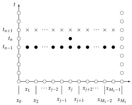
Figure 1.
Stencil of the numerical model (36) at the time in one spatial dimension. The black circles denote the known solutions at the times and . Meanwhile, the crosses represent the unknown approximations at the time . For the sake of convenience, we agree that .
We study the existence and uniqueness of solutions of the finite-difference method (36). To that end, we require some additional nomenclature and technical results. To start with, we let and , and fix the spatial mesh . Let be the complex vector space of all grid functions which vanish at the boundary of the mesh. For any and , convey that .
Definition 5.
Define the product and the norm by
The Euclidean norm induced by the inner product is denoted by .
In the following, we represent the solutions of the finite-difference method (36) by , where we agree that and , for each . We use the following lemma to prove that solutions of (36) exist.
Lemma 3
(Browder fixed-point theorem [23]). Let be a finite-dimensional inner-product space, let be the norm induced by the inner product, and suppose that is continuous. Assume that there exists such that , for all with . Then, there is , such that and .
Theorem 3
(Solubility). For any set of initial conditions, the discrete system (36) is solvable.
Proof.
The proof requires mathematical induction. Notice that the approximations at the times and are provided by the initial profiles and the explicit systems (37) and (38), respectively. Thus, let us suppose that the numerical solutions of the discrete model (36) at the times and n are known, for some . Rearranging the recursive equations of the method, we can readily check that the following equations hold:
and
for each . Define the function by , for each , where the functions are defined by
for each , , . After some calculations, we readily reach that
Using now the Cauchy–Schwarz inequality and bounding from below, it is easy to check that the following hold:
If we let in the previous lemma, it follows that there exists which satisfies the discrete system (36). The conclusion of this result readily follows now by induction. □
3. Structural Properties
The present section is devoted to showing that the discrete model (36) satisfies physical properties which are similar to those satisfied by the continuous system (4). More precisely, we propose numerical energy and mass functional associated to the scheme (36) which are conserved conditionally. Various technical lemmas are required to that end.
Lemma 4
(Macías-Díaz [24]). For each and , there exists a unique positive operator such that , for each .
Lemma 5.
The following equations hold, for each :
Proof.
To establish (48), notice that the following identities trivially hold:
To prove the identity (49), observe that
which establishes the second identity. We prove now the formula in part (51). To that end, notice that
Finally, we must point out that the proofs for the identities (50) and (52) are similar to the proofs of (49) and (51), respectively, and, for that reason, we omit them here. □
Lemma 6.
The following equations hold, for each and :
Proof.
Applying distributivity of the inner product and rearranging terms,
whence the first identity readily follows. To prove the second identity, we use once again the distributivity of the inner product and Lemma 4 to see that
which readily establishes the identity. Finally, using again distributivity and rearranging terms conveniently,
This last chain of identities readily establishes the last property of the lemma. □
The next theorem proves the existence of energy-like invariants for (36).
Theorem 4
Proof.
Denote the left-hand sides of the two difference equations in (36) by and , respectively, for each and , and define , . Using that is a solution of (36), calculating the inner product of with and of with , using the identities above and collecting terms, we reach
In similar fashion, notice that the following hold, for each :
Adding these two last identities, we readily obtain that , for each . The conclusion of this result is readily reached now using mathematical induction. □
Motivated by this result, the quantities are called the discrete total energy of the system (36) at the time , for each . In addition, we define the discrete energy density of the system (36) as
for each .
Lemma 7.
The following equations hold, for each and :
Proof.
Identity (a) readily follows from the fact that
which obviously yields zero. On the other hand, applying distributivity of the inner product on both factors, we obtain
which establishes Property (f). Finally, notice that distributivity also yields
which shows the validity of (g). The proofs of Properties (b)–(e) are similar to that of (a). For that reason, we omit the proofs of the remaining identities. □
Theorem 5
(Mass conservation). If is a solution of (36), then for each , where
is the discrete total mass of the system at the time . The discrete individual discrete masses as the quantities
and they are conserved if .
Proof.
Let and be as in the proof of Theorem 4, for each . Calculating the inner product of and with and , respectively, using the identities in the previous lemma. Collecting terms, we note that
and
for each . Observe that, indeed, the individual discrete masses are conserved if . On the other hand, adding the last two identities, we readily check that
for each , which is what we wanted to prove. □
After this last result, we refer to the quantities as the total mass of the discrete model (36) at the time , for each . Moreover, we define the density of mass at the point as the number
for each . It is worth noticing that the quantities and in the last theorems are clearly the discrete counterparts of the total energy and the total mass of associated to the continuous system (36), respectively.
Corollary 2
(Mass non-negativity). Let be a solution of (36), and suppose that . Then, the quantities are non-negative and constant.
Proof.
It only remains to prove that the quantities are non-negative. Using Young’s inequality, we obtain that
for each . This obviously completes the proof. □
The proof of the following result is similar to that of Corollary 2.
Corollary 3
(Boundedness). Suppose that is a solution of (36), and that satisfies . Then, , for each , □
4. Numerical Properties
To start with, we introduce the continuous functional
for each , and the next discrete functions, for each :
and
Using this nomenclature, we agree that
for each and .
Theorem 6
(Consistency). If , then there exist constants which are independent of h and τ, such that, for each , the following hold:
Proof.
Use Taylor’s theorem, Lemma 2 and the conditions of regularity, there are constants which are independent of h and , for , and , such that the next hold, for each :
The first inequality of the conclusion follows from the triangle inequality. The proof of the second inequality is similar. Finally, to prove the last inequality, observe firstly that the regularity conditions on and assure that there exist constants which are independent of h and , for , such that
The third inequality of this result readily follows now assuming that , using the triangle inequality, and letting be a suitable constant in terms of , and . □
Lemma 8
(Ferreira [25]). Let and be arrays of non-negative numbers for which there exists with the property that the following hold:
If , then . □
To prove stability, take two solutions of our scheme (36) associated to two sets of initial data. In notation, we assume that represents a solution for (36), and that solves the discrete problem but with initial profiles described by functions . Concretely, the following discrete initial-boundary-value problem holds:
for each .
Lemma 9.
Let and be sequences in . If then
Proof.
After substituting the definition of the operator at the left-hand side of the identity (103) and performing algebraic operations, we obtain that
Observe that most of the terms inside the sums cancel out. The conclusion readily follows now. □
Lemma 10.
Let and be solutions of (36) and (102), respectively, and let us define and , for each . For each , define
There is a constant which is independent of h and τ, such that, for each ,
Proof.
It is straightforward. □
Theorem 7
Proof.
Obviously, the next problem is satisfied, for each :
where and are as in Lemma 10. Then, there is independent of h and , with the property that, for each ,
Obtain the inner product of the first vector Equation of (110) with and calculate the imaginary parts. Meanwhile, in the second equation, obtain the inner product with and calculate imaginary parts. By Theorem 5,
It is readily checked then that that there exists independent of and h, such that
The conclusion of this result is reached now using Lemma 8. □
The following result is now straightforward.
Corollary 4
(Uniqueness). For any initial data, the problem (36) has a unique solution. □
We establish next the convergence properties of our finite-difference scheme. To that end, we assume that represents a pair of sufficiently smooth solutions of the initial-value problem (4). As a consequence,
Obviously, and represent here the local truncation errors.
Theorem 8
Proof.
Let be the solution of problem (36). For the sake of convenience, let us define and , for each . Notice that satisfies the problem
for each . Here, for each , we agree that
and
Using the regularity of and and Theorem 6, there exists a constant independent of and h, such that , for each . As in the previous theorem, there is independent of h and , such that
for each . This means that there is , such that, for each ,
From here, it is easy to reach the formulas
for each . Moreover, there exist independent of and h, such that
5. Numerical Simulations
The present section is devoted to describe our computational implementation of the finite-difference scheme (36), and to provide numerical simulations that illustrate the capability of the scheme to preserve the energy and the mass of the system. Our description of our implementation and the simulations are carried out in the one-dimensional case, that is, when . Moreover, for simplification purposes, let , , , and . Throughout this section, we represent the approximations in vector form as
For computational purposes, we define next various matrices, all of them with sizes equal to . To start with, we let and , for each , where , and are diagonal matrices defined through their diagonal entries by the formulas
and
and for each , we define
For each , we also introduce the matrices and , for each , where the new matrices and are diagonal, and they are defined as
and
Observe that the approximations at the times of the discrete model are provided exactly through the initial conditions in (36). Moreover, the approximations at the time are provided explicitly through Formulas (37) and (38). Meanwhile, the recursive equations of the discrete model can be alternatively expressed in terms of the nomenclature introduced in this work as
where the -dimensional vectors and are given by
It is worth pointing out that our computer implementation in Appendix A is based on the recursive system (134).
Example 1.

In the following, we use the constants in Table 1. Meanwhile, the parameters and change values between simulations, and , for each . On the other hand, , for each . Throughout, we fix the computer parameters and . In our simulations, we consider three cases for the differentiation orders and , namely,
Table 1.
Table of the parameter values employed in the numerical simulations of this work.
- Case 1.
- and .
- Case 2.
- and .
- Case 3.
- and .
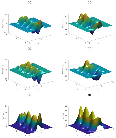
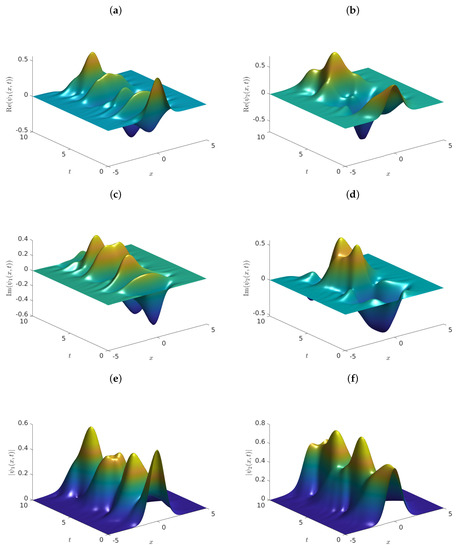
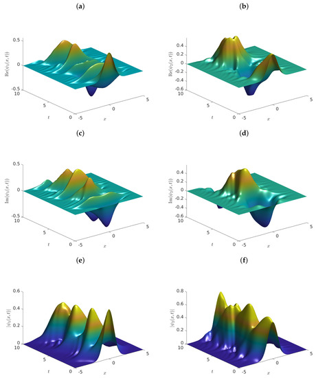
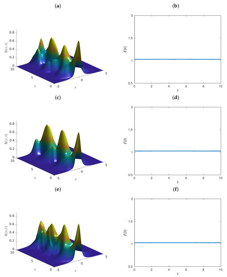
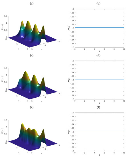
Under these circumstances, Figure 2, Figure 3 and Figure 4 provide the approximate solutions for the problem (4), using the values of Cases 1–3, respectively. In each figure, the graphs provide the behavior of the following, versus : (a) ; (b) ; (c) ; (d) ; (e) ; (f) . Figure 5 provides approximations for the energy functionals for these problems. More precisely, the left column of that figure provides approximate graphs of the discrete energy density versus , while the graphs of the total energy versus t are shown on the right column. We used Case 1 (top row), Case 2 (middle row) and Case 3 (bottom row). Obviously, the total energy of the system is approximately constant, as expected from the theoretical results. Finally, Figure 6 provides a similar analysis for the mass functionals of the mathematical model (4). The results show that the mass is approximately constant in all the cases, in agreement with the theoretical results proved in this manuscript.
Figure 2.
Approximate solutions for the problem (4) using the parameters in Table 1, and the computational time-steps and for the finite-difference method (36). We used , and initial data . The graphs provide the behavior of (a) , (b) , (c) , (d) , (e) , and (f) , versus . In these simulations, we used and .
Figure 3.
Approximate solutions for the problem (4) using the parameters in Table 1, and the computational time-steps and for the finite-difference method (36). We used , and initial data . The graphs provide the behavior of (a) , (b) , (c) , (d) , (e) , and (f) , versus . In these simulations, we used .
Figure 4.
Approximate solutions for the problem (4) using the parameters in Table 1, and the computational time-steps and for the finite-difference method (36). We used , and initial data . The graphs provide the behavior of (a) , (b) , (c) , (d) , (e) , and (f) , versus . In these simulations, we used and .
Figure 5.
Approximate solutions for the problem (4) using the parameters in Table 1, and the computational time-steps and for the finite-difference method (36). We used , and initial data . (left column) Approximate graphs of the discrete energy density versus . (right column) Graphs of the total energy versus t. We used and (a,b), and (c,d), and and (e,f).
Figure 6.
Approximate solutions for the problem (4) using the parameters in Table 1, and the computational time-steps and for the finite-difference method (36). We used , and initial data . (left column) Approximate graphs of the discrete mass density versus . (right column) Graphs of the total mass versus t. We used and (a,b), and (c,d), and and (e,f).
Example 2.
Next, we illustrate computationally the rate of convergence of (36). To that end, we use the values in Table 1 and the other parameters in the previous examples. Take a temporal period equal to and set . The exact solution of the problem is approximated letting and . Define and , for each . For convenience, define and . Let . Notice that
Introduce the convergence rates
and
Table 2 summarizes our computational investigation on the convergence of the scheme. The simulations show that (36) is quadratically convergent, as predicted by Theorem 8.
Table 2.
Table of absolute errors in the Euclidean norm and (a) temporal and (b) spatial rates of convergence for various values of the parameters and h. The experiment corresponds to that described in Example 2.
Before closing this section, it is important to point out that the extension of the Gross–Pitaevskii system to the fractional scenario (4) was proposed as a natural generalization of the classical Bose–Einstein condensates. Within that context and to the best of our knowledge, the theory of fractional operators has not found a solid justification via experimentation. However, the mathematical and numerical investigation of fractional extensions of this system is a difficult problem whose interest circumscribed to mathematical and numerical areas. Nevertheless, the authors hope that some potential applications of the present work will surface in the near future using some well-known applications of fractional derivatives (see Appendix B), and that the mathematical and numerical ideas developed in this work will lead to propose and analyze new computational methods for other physically relevant systems.
6. Conclusions
In this work, we study a finite-difference method for the coupled system of Gross–Pitaevskii equations with space-fractional derivatives in the Riesz sense. We prove the existence of solutions of our discretization for any set of initial conditions using a complex fixed-point theorem. Inspired by the existence of invariants in the continuous system, we show that some discrete forms of energy and mass functions are constant in time. As its continuous counterpart, we also prove the non-negativity of the mass function and the uniform boundedness of the approximations by imposing suitable numerical constraints. We present a rigorous numerical analysis for the method, obtaining a second order of consistency in space and time for the solutions. Moreover, we show that the discrete energy and mass densities are consistent approximations of the continuous functionals. We also provide conditions to guarantee the stability and the uniqueness of the numerical solutions, and we prove the convergence of the system. The theoretical results show that the method is quadratically convergent. It is worth pointing out that analyses of stability and convergence were carried out using a discrete version of Gronwall’s inequality. A Matlab implementation of the numerical model is provided in the Appendix of this work, and we used to produce approximations to the solutions of our continuous model. The results show that the energy and mass are approximately constant, in agreement with the theoretical results derived in this work, and improving computationally efforts already reported [20,26].
It is worth pointing out that there are already some reports by these same authors on the design of numerical methods to solve double Gross–Pitaevskii-type systems with fractional diffusion, most notably the papers by Serna-Reyes et al. [26] and Serna-Reyes and Macías-Díaz [20]. In both works, the same system of fractional partial differential equations is investigated using a finite-difference methodology, the fractional derivatives are of the Riesz type, and they are discretized using fractional-order centered differences. To start with, the proofs for the existence of solutions of the numerical model are more complicated in the case of the published papers [20,26]. Indeed, the arguments in those cases require using some fixed-point theorem in view of the nonlinear nature of those works. Meanwhile, in the present work, the existence of solutions is readily established using matrix arguments. This is due to the linear nature of the numerical solved. Moreover, the uniqueness in the present case is derived at the same time as the existence. In terms of conservation of energy, all the numerical models are capable of preserving this quantity except [26]. All the numerical models have a consistency of the second order in both space and time, and they are all stable and quadratically convergent in both space and time, for sufficiently small values of the computer parameters. Finally, in terms of implementation, the present numerical methodology is easy to implement computationally, in view that the code only requires solving a couple of linear systems at each time steps. On the other hand, the finite-difference schemes reported in [20,26] are harder to code. This is again due to the nonlinear nature of the numerical models. Since the solution functions are complex-valued, implementations of Newton’s method are useless in this point. To overcome this shortcoming, those methods were implemented using a recursive approach.
After the completion of this work, various avenues of research remain open in the investigation of fractional systems with associated energy functions. It is worth recalling that there are already various reports available in the literature on energy-conserving methods for a wide family of mathematical models and their fractional extensions [27,28]. Those fractional extensions have been mainly established for the case of Riesz space-fractional mathematical models [29]. Unfortunately, the property of energy conservation has not been studied in depth for Caputo time-fractional hyperbolic systems. There are very few reports in the literature which address this topic [30]. In fact, only some few reports for the parabolic case have shown some success in preserving the dissipation of free energy in those systems [31]. To this day, this problem remains open, and its solution is one of the avenues of research that should be tackled after the successful completion of so many on energy-conserving methods for space-fractional partial differential equations. In particular, the authors of this work are interested in developing dissipation-preserving methods for time-space-fractional extensions of the model investigated in the present manuscript, using Caputo fractional operators in time and Riesz fractional derivatives in space.
Author Contributions
Conceptualization, J.E.M.-D.; methodology, J.E.M.-D.; software, A.J.S.-R. and J.E.M.-D.; validation, A.J.S.-R. and J.E.M.-D.; formal analysis, A.J.S.-R. and J.E.M.-D.; investigation, J.E.M.-D.; resources, J.E.M.-D.; data curation, J.E.M.-D.; writing—original draft preparation, A.J.S.-R. and J.E.M.-D.; writing—review and editing, J.E.M.-D.; visualization, J.E.M.-D.; supervision, J.E.M.-D.; project administration, J.E.M.-D.; and funding acquisition, J.E.M.-D. All authors have read and agreed to the published version of the manuscript.
Funding
The first author (A.J.S.-R.) would like to acknowledge the financial support of the National Council for Science and Technology of Mexico (CONACYT). The corresponding author (J.E.M.-D.) acknowledges the financial support from CONACYT through grant A1-S-45928.
Institutional Review Board Statement
Not applicable.
Informed Consent Statement
Not applicable.
Data Availability Statement
The data that support the findings of this study are available from the corresponding author, J.E.M.-D., upon reasonable request.
Acknowledgments
The present manuscript is a submission to the Special Issue of Mathematics MDPI on “Fractional Calculus—Theory and Applications”. The authors would like to thank the anonymous reviewers and the associated editor in charge of handling this work for their time and comments. All of their suggestions were strictly followed, and the result was a substantial improvement in the final quality of this work.
Conflicts of Interest
The authors declare no conflict of interest.
Appendix A. Matlab Code
The following is a Matlab implementation of the finite-difference method (36), using the vector representation (134) for the recursive equations. It is important to point out here that we chose to provide a Matlab implementation of the numerical model in view that scientists are more familiarized with this computer language rather than with C/C++ or Fortran. However, the translation of this code to those programming languages is relatively straightforward for programmers with minimal knowledge of C/C++ or Fortran.
function [X,Y,phi1,phi2,H,R,t,Energy,Mass]=gp
function H=fracmatrix(M,alpha,h)
g=zeros(1,M);
g(1)=gamma(alpha+1)/gamma(0.5∗alpha+1)^2/h^alpha;
for l=1:M-1
g(l+1)=(1-(alpha+1)/(0.5∗alpha+l))∗g(l);
end
H=zeros(M,M);
for l=1:M
for m=1:M
H(l,m)=g(abs(l-m)+1);
end
end
end
a1=-5;
b1=5;
T=10;
alpha1=1.9;
alpha2=1.1;
beta11=1.5;
beta12=0.5;
beta22=1.5;
lambda=-0.5;
D=2;
tau=0.05;
h=0.1;
x=a1:h:b1;
t=0:tau:T;
M=length(x);
N=length(t);
Ha1=fracmatrix(M,alpha1,h);
Ha2=fracmatrix(M,alpha2,h);
Ha3=fracmatrix(M,0.5∗alpha1,h);
Ha4=fracmatrix(M,0.5∗alpha2,h);
V=0.5.∗x.^2;
u1=exp(-x.^2)./sqrt(pi);
v1=exp(-x.^2)./sqrt(pi);
u2=u1+1i.∗tau.∗(-0.5.∗u1∗Ha1-V.∗u1-D.∗u1-lambda.∗v1...
-(beta11.∗abs(u1).^2+beta12.∗abs(v1).^2).∗u1);
v2=v1+1i.∗tau.∗(-0.5.∗v1∗Ha2-V.∗v1-lambda.∗u1...
-(beta12.∗abs(u1).^2+beta22.∗abs(v1).^2).∗v1);
A1=diag(1i-tau.∗V-tau.∗D)-0.5.∗tau.∗Ha1;
A2=diag(1i+tau.∗V+tau.∗D)+0.5.∗tau.∗Ha1;
B1=diag(1i-tau.∗V)-0.5.∗tau.∗Ha2;
B2=diag(1i+tau.∗V)+0.5.∗tau.∗Ha2;
Energy=zeros(size(t));
Mass=zeros(size(t));
[X,Y]=meshgrid(x,t);
phi1=zeros(size(X));
phi2=zeros(size(X));
H=zeros(size(X));
R=zeros(size(X));
phi1(1,:)=u1;
phi1(2,:)=u2;
phi2(1,:)=v1;
phi2(2,:)=v2;
H(1,:)=0.25.∗(abs(u1∗Ha3).^2+abs(u2∗Ha3).^2+abs(v1∗Ha4).^2+abs(v2∗Ha4).^2) ...
+0.5.∗V.∗(abs(u1).^2+abs(u2).^2+abs(v1).^2+abs(v2).^2) ...
+0.5.∗D.∗(abs(u1).^2+abs(u2).^2)+0.5.∗beta11.∗abs(u1).^2.∗abs(u2).^2 ...
+0.5.∗beta22.∗abs(v1).^2.∗abs(v2).^2 ...
+0.5.∗beta12.∗(abs(u1).^2.∗abs(v2).^2+abs(v1).⌵2.∗abs(u2).^2) ...
+lambda.∗real(u1.∗conj(v2)+v1.∗conj(u2));
R(1,:)=abs(u1).^2+abs(u2).^2+abs(v1).^2+abs(v2).^2 ...
-lambda.∗tau.∗imag(u1.∗conj(v2)+v1.∗conj(u2));
Energy(1)=h∗sum(H(1,:));
Mass(1)=h∗sum(R(1,:));
for n=3:N
a=tau.∗(beta11.∗abs(u2).^2+beta12.∗abs(v2).^2);
b=tau.∗(beta12.∗abs(u2).^2+beta22.∗abs(v2).^2);
u3=linsolve(A1′-diag(a), (A2′+diag(a))∗u1′ + 2.∗lambda.∗tau.∗v2′ )′;
v3=linsolve(B1′-diag(b), (B2′+diag(b))∗v1′ + 2.∗lambda.∗tau.∗u2′ )′;
u1=u2;
u2=u3;
v1=v2;
v2=v3;
phi1(n,:)=u3;
phi2(n,:)=v3;
H(n-1,:)=0.25.∗(abs(u1∗Ha3).^2+abs(u2∗Ha3).^2+abs(v1∗Ha4).^2+abs(v2∗Ha4).^2) ...
+0.5.∗V.∗(abs(u1).^2+abs(u2).^2+abs(v1).^2+abs(v2).^2) ...
+0.5.∗D.∗(abs(u1).^2+abs(u2).^2)+0.5.∗beta11.∗abs(u1).^2.∗abs(u2).^2 ...
+0.5.∗beta22.∗abs(v1).^2.∗abs(v2).^2 ...
+0.5.∗beta12.∗(abs(u1).^2.∗abs(v2).^2+abs(v1).^2.∗abs(u2).^2) ...
+lambda.∗real(u1.∗conj(v2)+v1.∗conj(u2));
R(n-1,:)=abs(u1).^2+abs(u2).^2+abs(v1).^2+abs(v2).^2 ...
-lambda.∗tau.∗imag(u1.∗conj(v2)+v1.∗conj(u2));
Energy(n-1)=h∗sum(H(n-1,:));
Mass(n-1)=h∗sum(R(1,:));
end
Energy(N)=Energy(N-1);
Mass(N)=Mass(N-1);
H(N,:)=H(N-1,:);
R(N,:)=R(N-1,:);
end
Appendix B. Fractional Calculus
It is important to recall that Riesz space-fractional operators have been derived mathematically from physical systems with long-range interactions. Indeed, it has been established thoroughly that (parabolic or hyperbolic) partial differential equations with Riesz diffusion are obtained as the continuum limit of some particle systems with long-range interactions. This continuum-limit process involves the application of several operators, like Fourier series transform, the limit when the distance between consecutive particles goes to zero along with the inverse Fourier transform [32,33].
More precisely, suppose that s is a real number in the set and allow . We restrict our attention to the one-dimensional case and consider an array of particles on a straight line whose motion equations are described by the coupled system of ordinary differential equations
In this context, is a function that stands for the displacement of the nth particle with respect to the equilibrium point and F denotes the nonlinear interaction of the oscillators with some external force: Meanwhile, we use h to denote the distance existing between two consecutive oscillators. Moreover, a general form for the interaction function is fixed as
where is such that for each pair . For the sake of convenience, we introduce the function
and assume that the following is satisfied:
On both ends of (A1), apply the Fourier series transform. Next, take the limit and obtain finally the inverse Fourier transform. In such way, the following fractional partial differential equation is reached:
Here, the fractional derivative of order is understood in the sense of Riesz [32]. It is worth pointing out here that more details on these derivations are provided in [34].
References
- Adjabi, Y.; Jarad, F.; Baleanu, D.; Abdeljawad, T. On Cauchy problems with Caputo Hadamard fractional derivatives. J. Comput. Anal. Appl. 2016, 21, 661–681. [Google Scholar]
- Tan, W.; Jiang, F.L.; Huang, C.X.; Zhou, L. Synchronization for a class of fractional-order hyperchaotic system and its application. J. Appl. Math. 2012, 2012, 974639. [Google Scholar] [CrossRef]
- Zhou, X.; Huang, C.; Hu, H.; Liu, L. Inequality estimates for the boundedness of multilinear singular and fractional integral operators. J. Inequalities Appl. 2013, 2013, 1–15. [Google Scholar] [CrossRef]
- Liu, F.; Feng, L.; Anh, V.; Li, J. Unstructured-mesh Galerkin finite element method for the two-dimensional multi-term time–space fractional Bloch–Torrey equations on irregular convex domains. Comput. Math. Appl. 2019, 78, 1637–1650. [Google Scholar] [CrossRef]
- Hendy, A.S.; Macías-Díaz, J.E. A numerically efficient and conservative model for a Riesz space-fractional Klein–Gordon–Zakharov system. Commun. Nonlinear Sci. Numer. Simul. 2019, 71, 22–37. [Google Scholar] [CrossRef]
- Kilbas, A.A.; Srivastava, H.M.; Trujillo, J.J. Theory and Applications of Fractional Differential Equations; Elsevier: Amsterdam, The Netherlands, 2006; Volume 204. [Google Scholar]
- Cai, Z.; Huang, J.; Huang, L. Periodic orbit analysis for the delayed Filippov system. Proc. Am. Math. Soc. 2018, 146, 4667–4682. [Google Scholar] [CrossRef]
- Chen, T.; Huang, L.; Yu, P.; Huang, W. Bifurcation of limit cycles at infinity in piecewise polynomial systems. Nonlinear Anal. Real World Appl. 2018, 41, 82–106. [Google Scholar] [CrossRef]
- Wang, J.; Chen, X.; Huang, L. The number and stability of limit cycles for planar piecewise linear systems of node—Saddle type. J. Math. Anal. Appl. 2019, 469, 405–427. [Google Scholar] [CrossRef]
- Bai, L.; Liu, F.; Tan, S. A new efficient variational model for multiplicative noise removal. Int. J. Comput. Math. 2020, 97, 1444–1458. [Google Scholar] [CrossRef]
- Yuan, H. Convergence and stability of exponential integrators for semi-linear stochastic variable delay integro-differential equations. Int. J. Comput. Math. 2020, 98, 903–932. [Google Scholar] [CrossRef]
- Aldhaifallah, M.; Tomar, M.; Nisar, K.; Purohit, S. Some new inequalities for (k, s)-fractional integrals. J. Nonlinear Sci. Appl. 2016, 9, 5374–5381. [Google Scholar] [CrossRef]
- Houas, M. Certain Weighted Integral Inequalities Involving the Fractional Hypergeometric Operators. Sci. Ser. A Math. Sci. 2016, 27, 87–97. [Google Scholar]
- Houas, M. On some generalized integral inequalities for Hadamard fractional integrals. Med. J. Model. Simul. 2018, 9, 43–52. [Google Scholar]
- Baleanu, D.; Mohammed, P.O.; Vivas-Cortez, M.; Rangel-Oliveros, Y. Some modifications in conformable fractional integral inequalities. Adv. Differ. Equ. 2020, 2020, 1–25. [Google Scholar] [CrossRef]
- Abdeljawad, T.; Mohammed, P.O.; Kashuri, A. New modified conformable fractional integral inequalities of Hermite–Hadamard type with applications. J. Funct. Spaces 2020, 2020, 4352357. [Google Scholar] [CrossRef]
- Mohammed, P.O.; Abdeljawad, T. Integral inequalities for a fractional operator of a function with respect to another function with nonsingular kernel. Adv. Differ. Equ. 2020, 2020, 1–19. [Google Scholar] [CrossRef]
- Mohammed, P.O.; Brevik, I. A new version of the Hermite–Hadamard inequality for Riemann–Liouville fractional integrals. Symmetry 2020, 12, 610. [Google Scholar] [CrossRef]
- Podlubny, I. Fractional Differential Equations: An Introduction to Fractional Derivatives, Fractional Differential Equations, to Methods of Their Solution and Some of Their Applications; Mathematics in Science and Engineering; Academic Press: London, UK, 1999. [Google Scholar]
- Serna-Reyes, A.J.; Macías-Díaz, J. Theoretical analysis of a conservative finite-difference scheme to solve a Riesz space-fractional Gross—Pitaevskii system. J. Comput. Appl. Math. 2021, 113413. [Google Scholar] [CrossRef]
- Ortigueira, M.D. Riesz potential operators and inverses via fractional centred derivatives. Int. J. Math. Math. Sci. 2006, 2006, 48391. [Google Scholar] [CrossRef]
- Wang, X.; Liu, F.; Chen, X. Novel second-order accurate implicit numerical methods for the Riesz space distributed-order advection-dispersion equations. Adv. Math. Phys. 2015, 2015, 590435. [Google Scholar] [CrossRef]
- Farmakis, I.; Moskowitz, M. Fixed Point Theorems and Their Applications; World Scientific: Singapore, 2013. [Google Scholar]
- Macías-Díaz, J.E. An explicit dissipation-preserving method for Riesz space-fractional nonlinear wave equations in multiple dimensions. Commun. Nonlinear Sci. Numer. Simul. 2018, 59, 67–87. [Google Scholar] [CrossRef]
- Ferreira, R.A. A discrete fractional Gronwall inequality. Proc. Am. Math. Soc. 2012, 140, 1605–1612. [Google Scholar] [CrossRef]
- Serna-Reyes, A.J.; Macías-Díaz, J.E.; Reguera, N. A Convergent Three-Step Numerical Method to Solve a Double-Fractional Two-Component Bose–Einstein Condensate. Mathematics 2021, 9, 1412. [Google Scholar] [CrossRef]
- Macías-Díaz, J.; Medina-Ramírez, I. An implicit four-step computational method in the study on the effects of damping in a modified α-Fermi—Pasta—Ulam medium. Commun. Nonlinear Sci. Numer. Simul. 2009, 14, 3200–3212. [Google Scholar] [CrossRef]
- Macías-Díaz, J.E.; Puri, A. A numerical method with properties of consistency in the energy domain for a class of dissipative nonlinear wave equations with applications to a Dirichlet boundary-value problem. ZAMM-J. Appl. Math. Mech./Z. Angew. Math. Mech. Appl. Math. Mech. 2008, 88, 828–846. [Google Scholar] [CrossRef]
- Macías-Díaz, J.E. On the solution of a Riesz space-fractional nonlinear wave equation through an efficient and energy-invariant scheme. Int. J. Comput. Math. 2019, 96, 337–361. [Google Scholar] [CrossRef]
- Tarasov, V.E.; Zaslavsky, G.M. Conservation laws and Hamilton’s equations for systems with long-range interaction and memory. Commun. Nonlinear Sci. Numer. Simul. 2008, 13, 1860–1878. [Google Scholar] [CrossRef]
- Tang, T.; Yu, H.; Zhou, T. On energy dissipation theory and numerical stability for time-fractional phase-field equations. SIAM J. Sci. Comput. 2019, 41, A3757–A3778. [Google Scholar] [CrossRef]
- Tarasov, V.E. Continuous limit of discrete systems with long-range interaction. J. Phys. A Math. Gen. 2006, 39, 14895. [Google Scholar] [CrossRef]
- Tarasov, V.E. Lattice model of fractional gradient and integral elasticity: Long-range interaction of Grünwald–Letnikov–Riesz type. Mech. Mater. 2014, 70, 106–114. [Google Scholar] [CrossRef]
- Macías-Díaz, J.E. A numerically efficient dissipation-preserving implicit method for a nonlinear multidimensional fractional wave equation. J. Sci. Comput. 2018, 77, 1–26. [Google Scholar] [CrossRef]


Publisher’s Note: MDPI stays neutral with regard to jurisdictional claims in published maps and institutional affiliations. |
© 2021 by the authors. Licensee MDPI, Basel, Switzerland. This article is an open access article distributed under the terms and conditions of the Creative Commons Attribution (CC BY) license (https://creativecommons.org/licenses/by/4.0/).