Article

A New Forward–Backward Algorithm with Line Searchand Inertial Techniques for Convex Minimization Problems with Applications

by
Dawan Chumpungam
1,
Panitarn Sarnmeta
1 and
Suthep Suantai
1,2,*
1
Data Science Research Center, Department of Mathematics, Faculty of Science, Chiang Mai University, Chiang Mai 50200, Thailand
2
Research Center in Mathematics and Applied Mathematics, Department of Mathematics, Faculty of Science, Chiang Mai University, Chiang Mai 50200, Thailand
*
Author to whom correspondence should be addressed.
Mathematics 2021, 9(13), 1562; https://doi.org/10.3390/math9131562
Submission received: 17 May 2021 / Revised: 29 June 2021 / Accepted: 30 June 2021 / Published: 2 July 2021
(This article belongs to the Special Issue Nonlinear Problems and Applications of Fixed Point Theory)

Abstract

:
For the past few decades, various algorithms have been proposed to solve convex minimization problems in the form of the sum of two lower semicontinuous and convex functions. The convergence of these algorithms was guaranteed under the L-Lipschitz condition on the gradient of the objective function. In recent years, an inertial technique has been widely used to accelerate the convergence behavior of an algorithm. In this work, we introduce a new forward–backward splitting algorithm using a new line search and inertial technique to solve convex minimization problems in the form of the sum of two lower semicontinuous and convex functions. A weak convergence of our proposed method is established without assuming the L-Lipschitz continuity of the gradient of the objective function. Moreover, a complexity theorem is also given. As applications, we employed our algorithm to solve data classification and image restoration by conducting some experiments on these problems. The performance of our algorithm was evaluated using various evaluation tools. Furthermore, we compared its performance with other algorithms. Based on the experiments, we found that the proposed algorithm performed better than other algorithms mentioned in the literature.

1. Introduction

The convex minimization problem has been studied intensively for the past few decades due to its wide range of applications in various real-world problems. Some major problems in physics, economics, data science, engineering, and medical science can be viewed as convex minimization problems, for instance a reaction–diffusion equation, which is a mathematical model describing physical phenomena, such as chemical reactions, heat flow models, and population dynamics. The problem of finding an unknown reaction term of such an equation can be formulated as a coefficient inverse problem (CIP) for a partial differential equation (PDE). Numerical methods for solving CIPs for PDEs, as well as their applications to various subjects have been widely studied and analyzed; for more comprehensive information on this topic, see [1,2,3,4,5]. To obtain a globally convergent method for solving CIPs for PDEs, many authors have employed the convexification technique, which reformulates CIPs as convex minimization problems; for a more in-depth development and discussion, we refer to [6,7,8]. Therefore, a numerical method for convex minimization problems can be applied. More examples of convex minimization problems are signal and image processing, compressed sensing, and machine learning tasks such as regression and classification; see [9,10,11,12,13,14,15,16] and the references therein for more information.
The problem is formulated, in the form of the summation of two convex functions, as follows:
min x H { f ( x ) + g ( x ) } ,
where f , g : H R { + } are proper, lower semicontinuous convex functions and H is a Hilbert space.
If f is differentiable, then x solves (1) if and only if:
x = p r o x α g ( I α f ) ( x ) ,
where α > 0 , p r o x α g ( x ) = J α g ( x ) = ( I α g ) 1 ( x ) , I is an identity mapping and g is a subdifferential of g . In other words, x is a fixed point of p r o x α g ( I α f ) . Under some conditions, the Picard iteration converges to the solution. As a result, the forward–backward algorithm [17], which is defined as follows:
x n + 1 = p r o x α n g ( I α n f ) ( x n ) , for   all   n N ,
where α n is a suitable step size, converges to a solution of (1). Due to its simplicity, this method has been intensively studied and improved by many researchers; see [10,16,18] and the references therein for more information. One well-known method, which notably improves the convergence rate of (3), is the fast iterative shrinkage-thresholding algorithm (FISTA) introduced by Beck and Teboulle [19]. To the best of our knowledge, most of these works assumed that f is Lipschitz continuous. However, in general, such an assumption might be too strong, and finding a Lipschitz constant of f is sometimes difficult. To relax this strong assumption, Cruz and Nghia [20] proposed a line search technique and replaced the Lipschitz continuity assumption of f with weaker assumptions, as seen in the following conditions:
Assumption A1.
f , g are proper lower semicontinuous convex functions with d o m g d o m f ;
Assumption A2.
f is differentiable on an open set containing d o m g , and f is uniformly continuous on any bounded subset of d o m g and maps any bounded subset of d o m g to a bounded set in  H .
Note that if f is L-Lipschitz continuous, then A2 holds. They also established an algorithm using a line search technique and obtained a weak convergence result under Assumptions 1 and 2. In the same work, they also proposed an accelerated algorithm based on FISTA and a line search technique. They showed that this accelerated algorithm performed better than the other introduced algorithm.
Recently, inspired by [20], Kankam et al. [9] proposed a new line search technique and a new algorithm to solve (1). They conducted some experiments on signal processing and found that their method performed better than that of Cruz and Nghia [20].
In recent years, many authors have utilized the inertial technique in order to accelerate their algorithms. This was first introduced by Polyak [21] to solve smooth convex minimization problems. After that, many inertial-type algorithms were proposed and studied by many authors; see [22,23,24,25] and the references therein.
The algorithms introduced in [9,20] are easy to employ, since a Lipschitz constant of the gradient of an objective function f is not required to exist. Although the convergence of these algorithms is guaranteed, some improvements are still welcome, specifically utilizing an inertial technique in order to improve the performance. Hence, in this work, motivated by the works mentioned above, our main objective was to propose a new algorithm that utilizes both line search and inertial techniques to not only guarantee its convergence to a solution of (1) without assuming an L-Lipschitz continuity on f , but also to improve its performance by mean of an inertial technique. We established a weak convergence theorem under Assumptions 1 and 2. Moreover, a complexity theorem of this new algorithm was studied. Furthermore, we employed our proposed algorithm to solve an image restoration problem, as well as data classification problems. Then, we evaluated its performance and compared it with various other algorithms. The proposed method is also of great interest in solving nonlinear coefficient inverse problems for partial differential equations, along with other possible applications of convex minimization problems.
This work is organized as follows: In Section 2, we recall important definitions, lemmas that will be used in later sections, as well as various methods introduced in [9,19,20,22]. In Section 3, we introduce a new algorithm using new line search and inertial techniques and establish its weak convergence to a solution of (1). Moreover, the complexity of this method is also analyzed. In Section 4, in order to compare the performance of the studied algorithms, some numerical experiments on data classification problems and image restoration problem are conducted and discussed. In the last section, the brief conclusion of this paper is presented.

2. Preliminaries

Throughout this work, we denote x n x and x n x as { x n } converges strongly and weakly to x, respectively. For h : H R { + } , we also denote d o m h : = { x H : h ( x ) < + } .
First, we recall some methods for solving (1) introduced by many authors mentioned in Section 1.
The fast iterative shrinkage-thresholding algorithm (FISTA) was introduced by Beck and Teboulle[19] as follows (Algorithm 1).
Algorithm 1: FISTA.
1:
Input Given y 1 = x 0 R n , and t 1 = 1 , for n N ,
x n = p r o x 1 L g ( y n 1 L f ( y n ) ) , t n + 1 = 1 + 1 + 4 t n 2 2 , θ n = t n 1 t n + 1 , y n + 1 = x n + θ n ( x n x n 1 ) , n N ,
where L is a Lipschitz constant of f .
In 2016, Cruz and Nghia [20] introduced a line search step as follows (Algorithm 2).
Algorithm 2: Line Search 1 ( x , σ , θ , δ ) .
1:
Input Given x d o m g , σ > 0 , θ ( 0 , 1 ) , and δ ( 0 , 1 2 ) .
2:
Set α = σ .
3:
while α f ( p r o x α g ( x α f ( x ) ) ) f ( x ) > δ p r o x α g ( x α f ( x ) ) x do
4:
    Set  α = θ α
5:
end while
6:
Output α .
They asserted that Line Search 1 stops after finitely many steps and proposed the following algorithm (Algorithm 3).
Algorithm 3: Line Search 1 stops after finitely many steps.
1:
Input Given x 0 d o m g , σ > 0 , θ ( 0 , 1 ) , and δ ( 0 , 1 2 ) , for n N ,
x n + 1 = p r o x α n g ( I α n f ) ( x n ) ,
where α n : = Line Search 1 ( x n , σ , θ , δ ) .
They showed that a sequence generated by Algorithm 3 converges weakly to a solution of (1) under Assumptions 1 and 2.
Recently, Kankam et al. [9] proposed a new line search technique as follows (Algorithm 4).
Algorithm 4: Line Search 2 ( x , σ , θ , δ ) .
1:
Input Given x d o m g , σ > 0 , θ ( 0 , 1 ) , and δ > 0 . Set
L ( x , α ) = p r o x α g ( x α f ( x ) ) ,   and S ( x , α ) = p r o x α g ( L ( x , α ) α f ( L ( x , α ) ) ) .
2:
Set α = σ .
3:
while
α max { f ( S ( x , α ) ) f ( L ( x , α ) ) , f ( L ( x , α ) ) f ( x ) } > δ ( S ( x , α ) L ( x , α ) + L ( x , α ) x )
do
4:
    Set  α = θ α , L ( x , α ) = L ( x , θ α ) , S ( x , α ) = S ( x , θ α )
5:
end while
6:
Output α .
They proved that Line Search 2 stops at finitely many steps and introduced the following algorithm (Algorithm 5).
Algorithm 5: Line Search 2 stops at finitely many steps.
1:
Input Given x 0 d o m g , σ > 0 , θ ( 0 , 1 ) , and δ ( 1 , 1 8 ) , for n N ,
y n = p r o x γ n g ( x n γ n f ( x n ) ) , x n + 1 = p r o x γ n g ( y n γ n f ( y n ) ) ,
where γ n : = Line Search 2 ( x n , σ , θ , δ ) .
They established a weak convergence theorem for Algorithm 5, under Assumptions 1 and 2. As we can see, Algorithms 3 and 5 do not utilize an inertial step.
Inspired by Algorithm 1 (FISTA), Cruz and Nghia [20] also proposed the following accelerated algorithm (Algorithm 6).
Algorithm 6: Accelerated algorithm.
1:
Input Given x 0 , x 1 d o m g , α 1 > 0 , θ ( 0 , 1 ) , t 0 = 1 , and δ ( 0 , 1 2 ) , for n N ,
t n + 1 = 1 + 1 + 4 t n 2 2 , y n = x n + ( t n 1 t n + 1 ) ( x n x n 1 ) , y ˜ n = P d o m g ( y n ) , x n + 1 = p r o x α n g ( y ˜ n α n f ( y ˜ n ) ) ,
where α n : = Line Search 1 ( y ˜ n , α n 1 , θ , δ ) , and P is a metric projection.
They showed that Algorithm 6 has better complexity than Algorithm 3. However, the convergence to a solution of (1) is not guaranteed under the inertial parameter β n = t n 1 t n + 1 .
In 2019, Attouch and Cabot [22] analyzed the convergence rate of a method called the relaxed inertial algorithm (RIPA) for solving monotone inclusion problems, which is closely related to convex minimization problems. This method utilizes an inertial step x n + β n ( x n x n 1 ) to improve its performance. It was defined as follows (Algorithm 7).   
Algorithm 7: RIPA.
1:
Input Given x 0 , x 1 H , β n 0 , ρ n ( 0 , 1 ] , μ n > 0 , for n N ,
y n = x n + β n ( x n x n 1 ) , x n + 1 = ( 1 ρ n ) y n + ρ n J μ n A ( y n ) ,
where A is a maximal monotone operator and J μ n A ( y n ) = ( I + μ n A ) 1 .
Under mild restrictions of the control parameters, they showed that Algorithm 7 (RIPA) gives a fast convergence rate.
Next, we recall some important tools that will be used in the later sections.
Definition 1.
For x H , a subdifferential of h at x is defined as follows:
h ( x ) : = { u H : u , y x + h ( x ) h ( y ) , y H } .
The following can be found in [26].
Lemma 1 ([26]).
A subdifferential h is maximal monotone. Moreover, a graph of h , G p h ( h ) : = { ( u , v ) H × H : v h ( u ) } is demiclosed, i.e., for any sequence ( u n , v n ) G p h ( h ) such that { u n } converges weakly to u and { v n } converges strongly to v , we have ( u , v ) G p h ( h ) .
The proximal operator, p r o x g : H d o m g with p r o x g ( x ) = ( I + g ) 1 ( x ) , is single-valued with the full domain, and the following holds:
x p r o x α g x α g ( p r o x α g x ) ,   for   all   x H   and   α > 0 .
The following lemmas are crucial for the main results.
Lemma 2 ([27]).
Let H be a real Hilbert space. Then, the following hold, for all x , y H and α [ 0 , 1 ] :
(i) 
x ± y 2 = x 2 ± 2 x , y + y 2 ;
(ii) 
α x + ( 1 α ) y 2 = α x 2 + ( 1 α ) y 2 α ( 1 α ) x y 2 ;
(iii) 
x + y 2 x 2 + 2 y , x + y .
Lemma 3 ([16]).
Let { a n } and { β n } be sequences of non-negative real numbers such that:
a n + 1 ( 1 + β n ) a n + β n a n 1 ,   f o r   a l l   n N .
Then, the following holds:
a n + 1 K j = 1 n ( 1 + 2 β j ) ,   w h e r e   K = max { a 1 , a 2 } .
Moreover, if n = 1 + β n < + , then { a n } is bounded.
Lemma 4 ([27]).
Let { a n } , { b n } and { δ n } be sequences of non-negative real numbers such that:
a n + 1 ( 1 + δ n ) a n + b n ,   f o r   a l l   n N .
If n = 1 + δ n < + and n = 1 + b n < + , then lim n + a n exists.
Lemma 5 ([28]).
Let H be a Hilbert space and { x n } a sequence in H such that there exists a nonempty subset Ω of H satisfying the following:
(i) 
for any x * Ω , lim n x n x * exists;
(ii) 
every weak-cluster point of { x n } belongs to Ω .
Then, { x n } converges weakly to an element in Ω.

3. Main Results

In this section, we assume the existence of a solution of (1) and denote S * the set of all such solutions. We modify Line Search 2 as follows (Algorithm 8).
Algorithm 8: Line Search 3 ( x , σ , θ , δ ) .
1:
Input Given x d o m g , σ > 0 , θ ( 0 , 1 ) , and δ > 0 . Set
L ( x , α ) = p r o x α g ( x α f ( x ) ) ,   and S ( x , α ) = p r o x α g ( L ( x , α ) α f ( L ( x , α ) ) ) .
2:
Set α = σ .
3:
while
α 2 ( f ( S ( x , α ) ) f ( L ( x , α ) ) + f ( L ( x , α ) ) f ( x ) ) > δ ( S ( x , α ) L ( x , α ) + L ( x , α ) x ) ,
do
4:
    Set  α = θ α , L ( x , α ) = L ( x , θ α ) , S ( x , α ) = S ( x , θ α )
5:
end while
6:
Output α .
We know that Line Search 3 terminates at a lower step than Line Search 2, since:
α 2 ( f ( S ( x , α ) ) f ( L ( x , α ) ) + f ( L ( x , α ) ) f ( x ) ) α max { f ( S ( x , α ) ) f ( L ( x , α ) ) , f ( L ( x , α ) ) f ( x ) } .
Therefore, Line Search 3 stops after finitely many steps. We introduce an accelerated algorithm by utilizing Line Search 3 as follows (Algorithm 9).
Algorithm 9.
1:
Input Given x 0 , x 1 d o m   g , β n 0 , σ > 0 , θ   ( 0 , 1 )   and   δ   ( 0 , 1 8 ) ,   for   n N ,
x ^ n   =   x n + β n ( x n x n 1 ) , y n   =   P d o m   g x ^ n , z n   =   p r o x γ n g ( y n γ n f ( y n ) ) , x n + 1   =   p r o x γ n g ( z n γ n f ( z n ) ) ,
for y n : = Line Search 3( y n , σ , θ , δ ), and P d o m   g is a metric projection map onto d o m   g .
Next, we establish our first theorem.
Theorem 1.
Let H be a Hilbert space, f : H R { + } and g : H R { + } proper lower semicontinuous convex functions satisfying A1 and A2. Suppose that d o m g is closed and the following also hold, for all n N :
C1. 
γ n γ > 0 ;
C2. 
β n 0   a n d   n = 1 + β n < + .
Then, a sequence { x n } generated by Algorithm 9 converges weakly to a point in S * .
Proof. 
For any x d o m g and n N , we claim that:
y n x 2 x n + 1 x 2 2 γ n [ ( f + g ) ( z n ) + ( f + g ) ( x n + 1 ) 2 ( f + g ) ( x ) ] + ( 1 8 δ ) ( z n y n 2 + x n + 1 z n 2 ) .
To prove our claim, we know, from (4) and the definition of g , that:
y n z n γ n f ( y n ) g ( z n ) ,   and z n x n + 1 γ n f ( z n ) g ( x n + 1 ) .
Then,
g ( x ) g ( z n ) y n z n γ n f ( y n ) , x z n ,   and
g ( x ) g ( x n + 1 ) z n x n + 1 γ n f ( z n ) , x x n + 1 ,   for   all   n N .
Moreover,
f ( x ) f ( y n ) f ( y n ) , x y n ,
f ( x ) f ( z n ) f ( z n ) , x z n ,
f ( y n ) f ( z n ) f ( z n ) , y n z n ,   and
f ( z n ) f ( x n + 1 ) f ( x n + 1 ) , z n x n + 1 ,   for   all   n N .
From the definition of γ n and the above inequalities, we have, for all x d o m g and n N ,
f ( x ) f ( y n ) + f ( x ) f ( z n ) + g ( x ) g ( z n ) + g ( x ) g ( x n + 1 ) 1 γ n y n z n , x z n + f ( y n ) , z n y n + 1 γ n z n x n + 1 , x x n + 1 + f ( z n ) , x n + 1 z n = 1 γ n y n z n , x z n + f ( y n ) f ( z n ) , z n y n + f ( z n ) , z n y n + 1 γ n z n x n + 1 , x x n + 1 + f ( z n ) f ( x n + 1 ) , x n + 1 z n + f ( x n + 1 ) , x n + 1 z n 1 γ n y n z n , x z n + 1 γ n z n x n + 1 , x x n + 1 f ( z n ) f ( y n ) z n y n + f ( z n ) , z n y n f ( x n + 1 ) f ( z n ) x n + 1 z n + f ( x n + 1 ) , x n + 1 z n 1 γ n y n z n , x z n + 1 γ n z n x n + 1 , x x n + 1 + f ( z n ) , z n y n f ( z n ) f ( y n ) ( z n y n + x n + 1 z n ) f ( x n + 1 ) f ( z n ) ( z n y n + x n + 1 z n ) + f ( x n + 1 ) , x n + 1 z n = 1 γ n y n z n , x z n + 1 γ n z n x n + 1 , x x n + 1 + f ( z n ) , z n y n + f ( x n + 1 ) , x n + 1 z n ( f ( z n ) f ( y n ) + f ( x n + 1 ) f ( z n ) ) ( z n y n + x n + 1 z n ) 1 γ n y n z n , x z n + 1 γ n z n x n + 1 , x x n + 1 + f ( z n ) , z n y n + f ( x n + 1 ) , x n + 1 z n 2 δ γ n ( z n y n + x n + 1 z n ) 2 1 γ n y n z n , x z n + 1 γ n z n x n + 1 , x x n + 1 + f ( x n + 1 ) f ( y n ) 4 δ γ n ( z n y n 2 + x n + 1 z n 2 ) .
Hence,
1 γ n y n z n , z n x + 1 γ n z n x n + 1 , x n + 1 x ( f + g ) ( z n ) + ( f + g ) ( x n + 1 ) 2 ( f + g ) ( x ) 4 δ γ n z n y n 2 4 δ γ n x n + 1 z n 2 .
Moreover, the following also hold, for all n N ,
y n z n , z n x = 1 2 ( y n x 2 y n z n 2 z n x 2 ) , a n d ,
z n x n + 1 , x n + 1 x = 1 2 ( z n x 2 z n x n + 1 2 x n + 1 x 2 ) .
As a result, we obtain:
1 2 γ n ( y n x 2 y n z n 2 ) 1 2 γ n ( z n x n + 1 2 + x n + 1 x 2 ) ( f + g ) ( z n ) + ( f + g ) ( x n + 1 ) 2 ( f + g ) ( x ) 4 δ γ n z n y n 2 4 δ γ n x n + 1 z n 2 ,
for all x d o m g and n N . Therefore,
y n x 2 x n + 1 x 2 2 γ n [ ( f + g ) ( z n ) + ( f + g ) ( x n + 1 ) 2 ( f + g ) ( x ) ] + ( 1 8 δ ) ( z n y n 2 + x n + 1 z n 2 ) ,
for all x d o m g and n N . Furthermore, putting x = x * S * , we obtain:
y n x * 2 x n + 1 x * 2 ( 1 8 δ ) ( z n y n 2 + x n + 1 z n 2 ) .
Next, we show that lim n x n x * exists. From (6), we have:
x n + 1 x * y n x * , = P d o m g x ^ n P d o m g x * , x ^ n x * , x n x * + β n x n x n 1 , ( 1 + β n ) x n x * + β n x n 1 x * , for   all   n N .
This implies by Lemma 3 and C2 that { x n } is bounded.
Consequently, n = 1 + β n x n x n 1 < + , and:
x ^ n x n = β n x n x n 1 0 , a s n + .
By (7) and Lemma 4, we obtain that lim n + x n x * exists. By the definitions of z n 1 and x n , we see x n d o m g , for all n N . As a result, we have:
x ^ n y n x ^ n x n , for   all   n N ,
so, lim n + x ^ n y n = 0 .
Thus, we obtain from (7) that lim n + x n x * = lim n + y n x * . Moreover, it follows from (6) that lim n + z n y n = 0 , and hence, lim n + z n x n = 0 .
Now, we prove that every weak-cluster point of { x n } belongs to S * . In order to accomplish this, we first let w be a weak-cluster point of { x n } . Therefore, there exists a subsequence { x n k } of { x n } such that x n k w , and hence, z n k w . Next, we prove that w belongs to S * . Since f is uniformly continuous, we have lim k + f z n k f y n k = 0 . From (4), we obtain:
y n k γ n k f y n k z n k γ n k g ( z n k ) , for   all   k N .
Hence,
y n k z n k γ n k f y n k + f z n k g ( z n k ) + f z n k = ( f + g ) ( z n k ) ,   for   all   k N .
By letting k + in the above inequality, the demiclosedness of G p h ( ( f + g ) ) implies that 0 ( f + g ) ( w ) , and hence, w S * . Therefore, every weak-cluster point of { x n } belongs to S * .
We derive from Lemma 5 that { x n } converges weakly to w * in S * . Therefore, { x n } converges weakly to a solution of (1), and the proof is complete. □
In the next theorem, we provide the complexity theorem of Algorithm 9. First, we introduce the control sequence { t n } defined in [22] by:
t n = 1 + k = n + ( i = n k β i ) ,   for   all   n N .
This sequence is well defined if the following assumption holds:
k = n + ( i = n k β i ) < + ,   for   all   n N .
Hence, from (8), we can see that:
β n t n + 1 = t n 1 ,   for   all   n N .
Next, we establish the following theorem.
Theorem 2.
Given x 0 = x 1 d o m g and letting { x n } be a sequence generated by Algorithm 9, assume that all assumptions in Theorem 1 are satisfied. Furthermore, suppose that the following conditions hold, for all n N :
D1. 
k = n + ( i = n k β i ) < + , and 2 t n + 1 2 2 t n + 1 t n 2 ,
D2. 
γ n γ n + 1 .
Then,
( f + g ) ( x n + 1 ) min x H ( f + g ) ( x ) d ( x 1 , S * ) 2 + 2 γ 1 t 1 2 [ ( f + g ) ( x 1 ) min x H ( f + g ) ( x ) ] 2 γ t n + 1 2 ,
for all n N . In other words,
( f + g ) ( x n + 1 ) min x H ( f + g ) ( x ) = O ( 1 t n + 1 2 ) , f o r a l l n N .
Proof. 
For any x d o m g , we know that:
y n x 2 x n + 1 x 2 2 γ n [ ( f + g ) ( z n ) + ( f + g ) ( x n + 1 ) 2 ( f + g ) ( x ) ]
for all n N . Since x d o m g , we obtain x ^ n x y n x . Thus, we conclude that:
x ^ n x 2 x n + 1 x 2 2 γ n [ ( f + g ) ( z n ) + ( f + g ) ( x n + 1 ) 2 ( f + g ) ( x ) ] , for   all   n N .
Let x * be an element in S * . We know that x n , x d o m g and t n + 1 1 , so ( 1 1 t n + 1 ) x n + 1 t n + 1 x * d o m g . Next, we put x = ( 1 1 t n + 1 ) x n + 1 t n + 1 x * in (10) and obtain the following:
x n + 1 ( 1 1 t n + 1 ) x n 1 t n + 1 x * 2 x ^ n ( 1 1 t n + 1 ) x n 1 t n + 1 x * 2 2 γ n [ ( f + g ) ( ( 1 1 t n + 1 ) x n + 1 t n + 1 x * ) ( f + g ) ( x n + 1 ) ] + 2 γ n [ ( f + g ) ( ( 1 1 t n + 1 ) x n + 1 t n + 1 x * ) ( f + g ) ( z n ) ] 2 γ n [ ( 1 1 t n + 1 ) ( f + g ) ( x n ) + 1 t n + 1 ( f + g ) ( x * ) ( f + g ) ( x n + 1 ) ] + 2 γ n [ ( 1 1 t n + 1 ) ( f + g ) ( x n ) + 1 t n + 1 ( f + g ) ( x * ) ( f + g ) ( z n ) ] = 2 γ n [ ( 1 1 t n + 1 ) [ ( f + g ) ( x n ) ( f + g ) ( x * ) ] [ ( f + g ) ( x n + 1 ) ( f + g ) ( x * ) ] ] + 2 γ n [ ( 1 1 t n + 1 ) [ ( f + g ) ( x n ) ( f + g ) ( x * ) ] [ ( f + g ) ( z n ) ( f + g ) ( x * ) ] ] 4 γ n ( 1 1 t n + 1 ) [ ( f + g ) ( x n ) ( f + g ) ( x * ) ] 2 γ n [ ( f + g ) ( x n + 1 ) ( f + g ) ( x * ) ] ,
for all n N . From D1 and D2, we know that t n 2 2 t n + 1 2 2 t n + 1 and γ n γ n + 1 , so:
4 γ n ( 1 1 t n + 1 ) [ ( f + g ) ( x n ) ( f + g ) ( x * ) ] 2 γ n [ ( f + g ) ( x n + 1 ) ( f + g ) ( x * ) ] 1 t n + 1 2 [ 2 γ n ( 2 t n + 1 2 2 t n + 1 ) [ ( f + g ) ( x n ) ( f + g ) ( x * ) ] 2 γ n + 1 t n + 1 2 [ ( f + g ) ( x n + 1 ) ( f + g ) ( x * ) ] ] 1 t n + 1 2 [ 2 γ n t n 2 [ ( f + g ) ( x n ) ( f + g ) ( x * ) ] 2 γ n + 1 t n + 1 2 [ ( f + g ) ( x n + 1 ) ( f + g ) ( x * ) ] ] , f o r a l l n N .
Moreover, we also have:
x n + 1 ( 1 1 t n + 1 ) x n 1 t n + 1 x * 2 x ^ n ( 1 1 t n + 1 ) x n 1 t n + 1 x * 2 = 1 t n + 1 2 ( t n + 1 x n + 1 ( t n + 1 1 ) x n x * 2 t n + 1 x n + β n t n + 1 ( x n x n 1 ) ( t n + 1 1 ) x n x * 2 ) = 1 t n + 1 2 ( t n + 1 x n + 1 ( t n + 1 1 ) x n x * 2 ( t n 1 ) ( x n x n 1 ) + x n x * 2 ) = 1 t n + 1 2 ( t n + 1 x n + 1 ( t n + 1 1 ) x n x * 2 t n x n ( t n 1 ) x n 1 x * 2 ) ,
for all n N . By (11)–(13), we obtain:
t n + 1 x n + 1 ( t n + 1 1 ) x n x * 2 t n x n ( t n 1 ) x n 1 x * 2 2 γ n t n 2 [ ( f + g ) ( x n ) ( f + g ) ( x * ) ] 2 γ n + 1 t n + 1 2 [ ( f + g ) ( x n + 1 ) ( f + g ) ( x * ) ] ,
for all n N . It follows that:
2 γ n + 1 t n + 1 2 [ ( f + g ) ( x n + 1 ) ( f + g ) ( x ) ] t n x n ( t n 1 ) x n 1 x * 2 t n + 1 x n + 1 ( t n + 1 1 ) x n x * 2 + 2 γ n t n 2 [ ( f + g ) ( x n ) ( f + g ) ( x * ) ] ,
for all n N . Moreover, we can inductively prove, from (14), that:
2 γ n + 1 t n + 1 2 [ ( f + g ) ( x n + 1 ) ( f + g ) ( x * ) ] t n x n ( t n 1 ) x n 1 x * 2 + 2 γ n t n 2 [ ( f + g ) ( x n ) ( f + g ) ( x * ) ] t n 1 x n 1 ( t n 1 1 ) x n 2 x * 2 + 2 γ n 1 t n 1 2 [ ( f + g ) ( x n 1 ) ( f + g ) ( x * ) ] t 1 x 1 ( t 1 1 ) x 0 x * 2 + 2 γ 1 t 1 2 [ ( f + g ) ( x 1 ) ( f + g ) ( x * ) ] ,
for all n N . From C1, we know that γ n + 1 γ . Therefore, we obtain, for all n N ,
( f + g ) ( x n + 1 ) min x H ( f + g ) ( x ) 1 2 γ n + 1 t n + 1 2 x 1 x * 2 + 2 γ 1 t 1 2 2 γ n + 1 t n + 1 2 [ ( f + g ) ( x 1 ) ( f + g ) ( x * ) ] x 1 x * 2 + 2 γ 1 t 1 2 [ ( f + g ) ( x 1 ) min x H ( f + g ) ( x ) ] 2 γ t n + 1 2 .
Since x * is arbitrarily chosen from S * , we have:
( f + g ) ( x n + 1 ) min x H ( f + g ) ( x ) d ( x 1 , S * ) 2 + 2 γ 1 t 1 2 [ ( f + g ) ( x 1 ) min x H ( f + g ) ( x ) ] 2 γ t n + 1 2 ,
for all n N , and the proof is complete. □
Remark 1.
To justify that there exists a sequence { β n } satisfying D1, we choose:
β n = 1 ( n + 1 ) 2 , for   all   n N .
We see that, for all n N ,
t n = 1 + 1 ( n + 1 ) 2 + 1 ( n + 1 ) 2 ( n + 2 ) 2 + 1 ( n + 1 ) 2 ( n + 2 ) 2 ( n + 3 ) 2 +   .
Therefore, we have:
t n + 1 t n for   all   n N .
Furthermore, it can be seen that t n + 1 < 1 + k = 3 + 1 k 2 = π 2 6 1 4 , for all n N . Then:
2 t n + 1 2 2 t n + 1 = ( t n + 1 ) ( 2 t n + 1 2 ) ( t n ) ( π 2 3 5 2 ) , f o r a l l n N .
Since π 2 3 5 2 < 1 , we can conclude that
2 t n + 1 2 2 t n + 1 < t n < t n 2 ,
for all n N . Obviously, k = n + ( i = n k β i ) < + ; , hence D1 is satisfied.
We also note that to obtain a sequence { γ n } satisfying D2, one could simply modify Algorithm 9 by choosing γ n = Line Search 3 ( y n , γ n 1 , θ , δ ) .

4. Applications to Data Classification and Image Restoration Problems

In this section, the proposed algorithm is used to solve classification and image restoration problems. The performance of Algorithm 9 is evaluated and compared with Algorithms 3, 5, and 6.

4.1. Data Classification

Data classification is a major branch of problems in machine learning, which is an application of artificial intelligence (AI) possessing the ability to learn and improve from experience without being programmed. In this work, we focused on one particular learning technique called extreme learning machine (ELM) introduced by Huang et al. [29]. It is defined as follows.
Let S : = { ( x k , t k ) : x k R n , t k R m , k = 1 , 2 , . . . , N } be a training set of N samples, where x k is an input and t k is a target. The output of ELM with M hidden nodes and activation function G is defined by:
o j = i = 1 M η i G ( w i , x j + b i ) ,
where w i is the weight vector connecting the i-th hidden node and the input node, η i is the weight vector connecting the i-th hidden node and the output node, and b i is the bias. The hidden layer output matrix H is formulated as:
H = G ( w 1 , x 1 + b 1 ) G ( w M , x 1 + b M ) G ( w 1 , x N + b 1 ) G ( w M , x N + b M ) .
The main goal of ELM is to find an optimal weight η = [ η 1 T , . . . , η M T ] T such that H η = T , where T = [ t 1 T , . . . , t N T ] T is the training set. If the Moore–Penrose generalized inverse H of H exists, then η = H T is the desired solution. However, in general cases, H may not exist or be challenging to find. Hence, to avoid such difficulties, we applied the concept of convex minimization to find η without relying on H .
To prevent overfitting, we used the least absolute shrinkage and selection operator (LASSO) [30], formulated as follows:
min η { H η T 2 2 + λ η 1 } ,
where λ is a regularization parameter. In the setting of convex minimization, we set f ( x ) = H x T 2 2 and g ( x ) = λ x 1 .
In the experiment, we aimed to classify three datasets https://archive.ics.uci.edu, accessed on 1 May 2021.
Iris dataset [31]: Each sample in this dataset has four attributes, and the set contains three classes with fifty samples for each type.
Heart disease dataset [32]: This dataset contains 303 samples, each of which has 13 attributes. In this dataset, we classified two classes of data.
Wine dataset [33]: In this dataset, we classified three classes of one-hundred seventy-eight samples. Each sample contained 13 attributes.
In all experiments, we used the sigmoid as the activation function with the number of hidden nodes M = 30 . The accuracy of the output is calculated by:
accuracy   =   correctly   predicted   data all   data × 100 .
We also utilized 10-fold cross-validation to evaluate the performance of each algorithm and used the average accuracy as the evaluation tool. It is defined as follows:
Average   ACC = i = 1 N x i y i × 100 % / N .
where N is the number of sets considered during cross-validation ( N = 10 ), x i is the number of correctly predicted data at fold i, and y i is the number of all data at fold i.
We used 10-fold cross-validation to split the data into training sets and testing sets; more information can be seen in Table 1.
All parameters of Algorithms 3, 5, 6 and 9 were chosen as in Table 2.
The inertial parameters β n of Algorithm 9 may vary depending on the dataset, since some β n work well on specific datasets. We used the following two choices of β n in our experiments.
β n 1 = 10 8 x n x n 1 3 + n 3 + 10 8 ,   and   β n 2 = 0.9 ,   if   n 1000 1 ( n + 1 ) 2 ,   if   n 1001 .
The regularization parameters λ for each dataset and algorithm were chosen to prevent overfitting, i.e., a model obtained from the algorithm achieves high accuracy on the training set, but low accuracy on the testing set in comparison, so it cannot be used to predict the unknown data. It is known that when λ is too large, the model tends to underfit, i.e., low accuracy on the training set, and cannot be used to predict the future data. On the other hand, if λ is too small, then it may not be enough to prevent a model from overfitting. In our experiment, for each algorithm, we chose a set of λ that satisfies | A c c _ t r a i n A c c _ t e s t | < 2 % , where A c c _ t r a i n and A c c _ t e s t are the average accuracy of the training set and testing set, respectively. Under this criterion, we can prevent the studied models from overfitting. Then, from these candidates, we chose λ , which yields high A C C _ t e s t for each algorithm. Therefore, the models obtained from Algorithms 3, 5, 6 and 9 can be effectively used to predict the unknown data.
By this process, the regularization parameters λ for Algorithms 5, 6, and 9 were as in Table 3.
We assessed the performance of each algorithm at the 300th iteration with the average accuracy. The results can be seen in Table 4.
As we see from Table 4, from the choice of λ , all models obtained from Algorithms 3, 5, 6 and 9 had reasonably high average accuracy on both the training and testing sets for all datasets. Moreover, we observed that a model from Algorithm 9 performed better than the models from other algorithms in terms of the accuracy in all experiments conducted.

4.2. Image Restoration

We first recall that an image restoration problem can be formulated as a simple mathematical model as follows:
A x = b + w
where x R n × 1 is the original image, A R m × n is a blurring matrix, b is an observed image, and w is noise. The main objective of image restoration is to find x from given image b , blurring matrix A, and noise w.
In order to solve (16), one could implement LASSO [30] and reformulate the problem in the following form.
min x { A x b 2 2 + λ x 1 } ,
where λ is a regularization parameter. Hence, it can be viewed as a convex minimization problem. Therefore, Algorithms 3, 5, 6 and 9 can be used to solve an image restoration problem.
In our experiment, we used the 256 × 256 color image as the original image. We used Gaussian blur of size 9 2 and standard deviation four on the original image and obtained the blurred image. In order to assess the performance of each algorithm, we implemented the peak-signal-to-noise ratio (PSNR) [34] defined by:
P S N R ( x n ) = 10 log 10 ( 255 2 MSE ) .
For any original image x and deblurred image x n , the mean squared error (MSE) is calculated by MSE   =   1 M x n x 2 , where M is the number of pixels of x. We also need to mention that an algorithm with a higher PSNR performs better than one with a lower PSNR.
The control parameters of each algorithm were chosen as δ = θ = σ = 0.1 . As the inertial parameter β n of Algorithm 9, we used the following:
β n = 0.95 ,   if   n 1000 1 n 2 ,   if   n 1001 . .
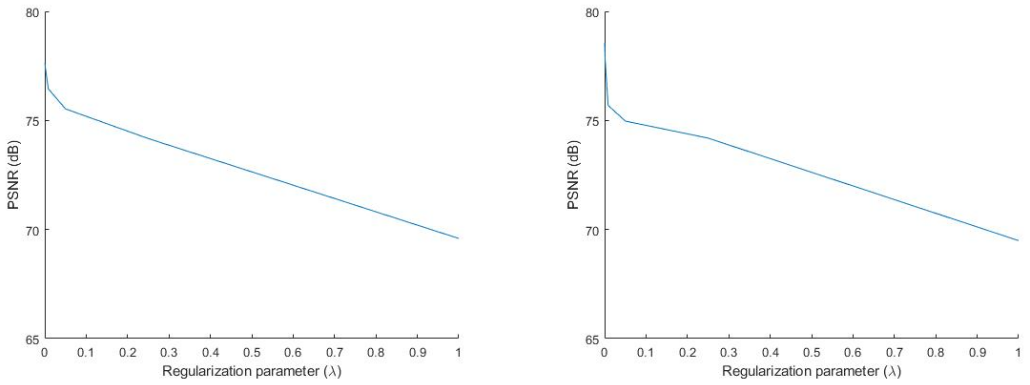
As for the regularization parameter λ , we experimented on λ varying from zero to one for each algorithm. In Figure 1, we show the PSNR of Algorithms 3 and 5 with respect to λ 
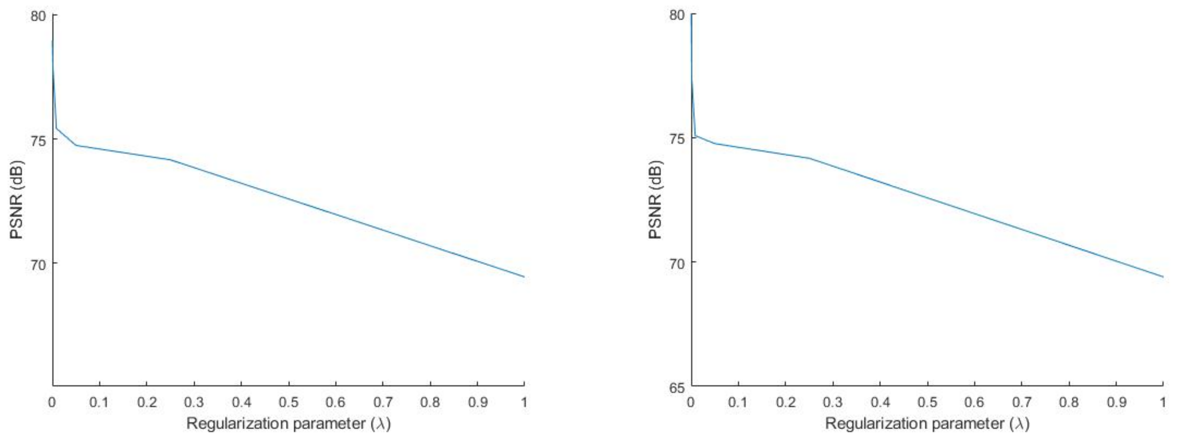
at the 200th iteration. In Figure 2, we show the PSNR of Algorithms 6 and 9 with respect to λ at the 200th iteration.
We observe from Figure 1 and Figure 2 that the PSNRs of Algorithms 3, 5, 6 and 9 increased as λ became smaller. Based on this, for the next two experiments, we chose λ 
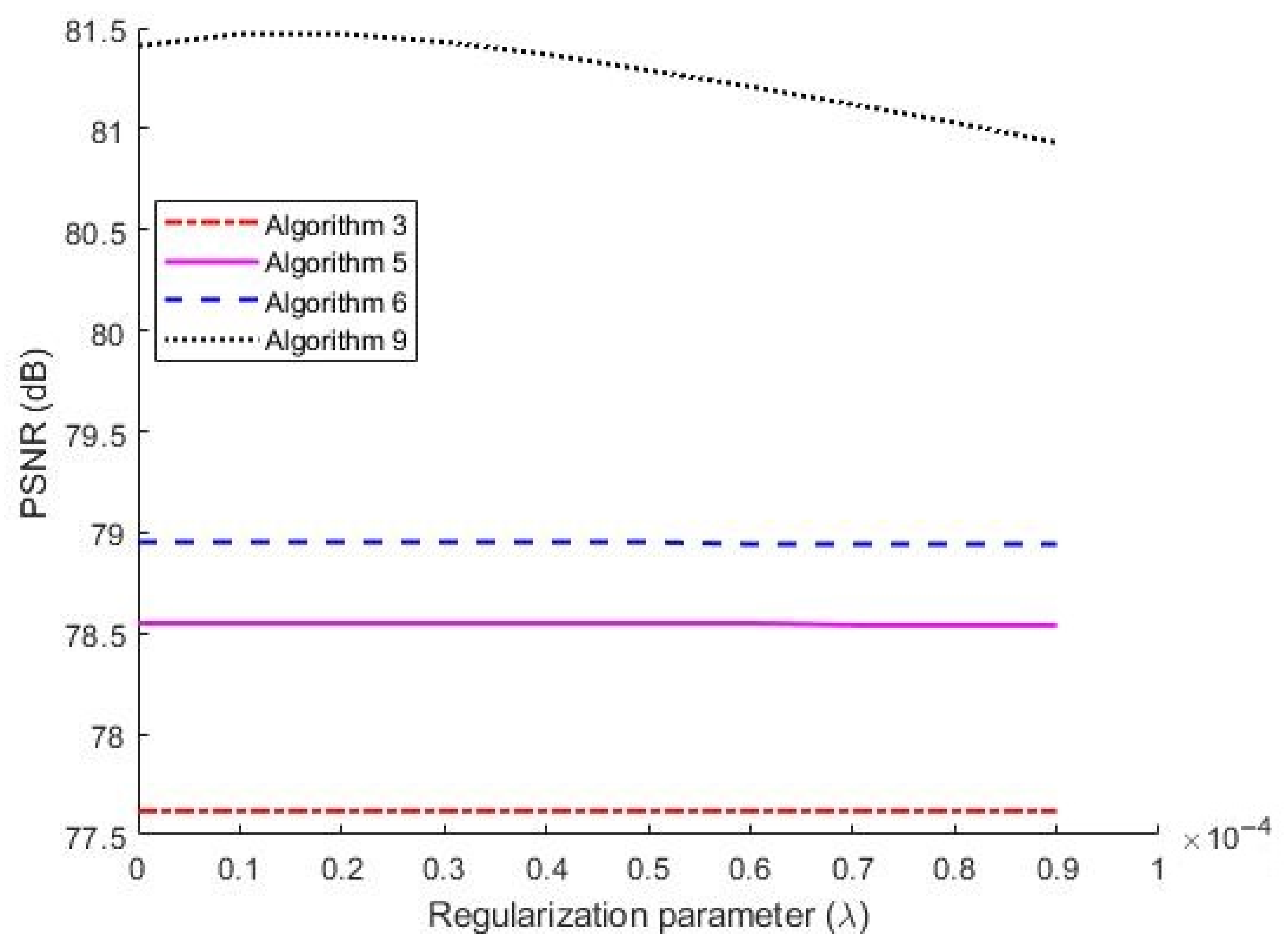
to be small to obtain a high PSNR for all algorithms. Next, we observed the PSNR of each algorithm when λ was small ( λ < 10 4 ). In Figure 3, we show the PSNR of each algorithm with respect to λ < 10 4 at the 200th iteration.
We see from Figure 3 that Algorithm 9 offered a higher PSNR than the other algorithms.
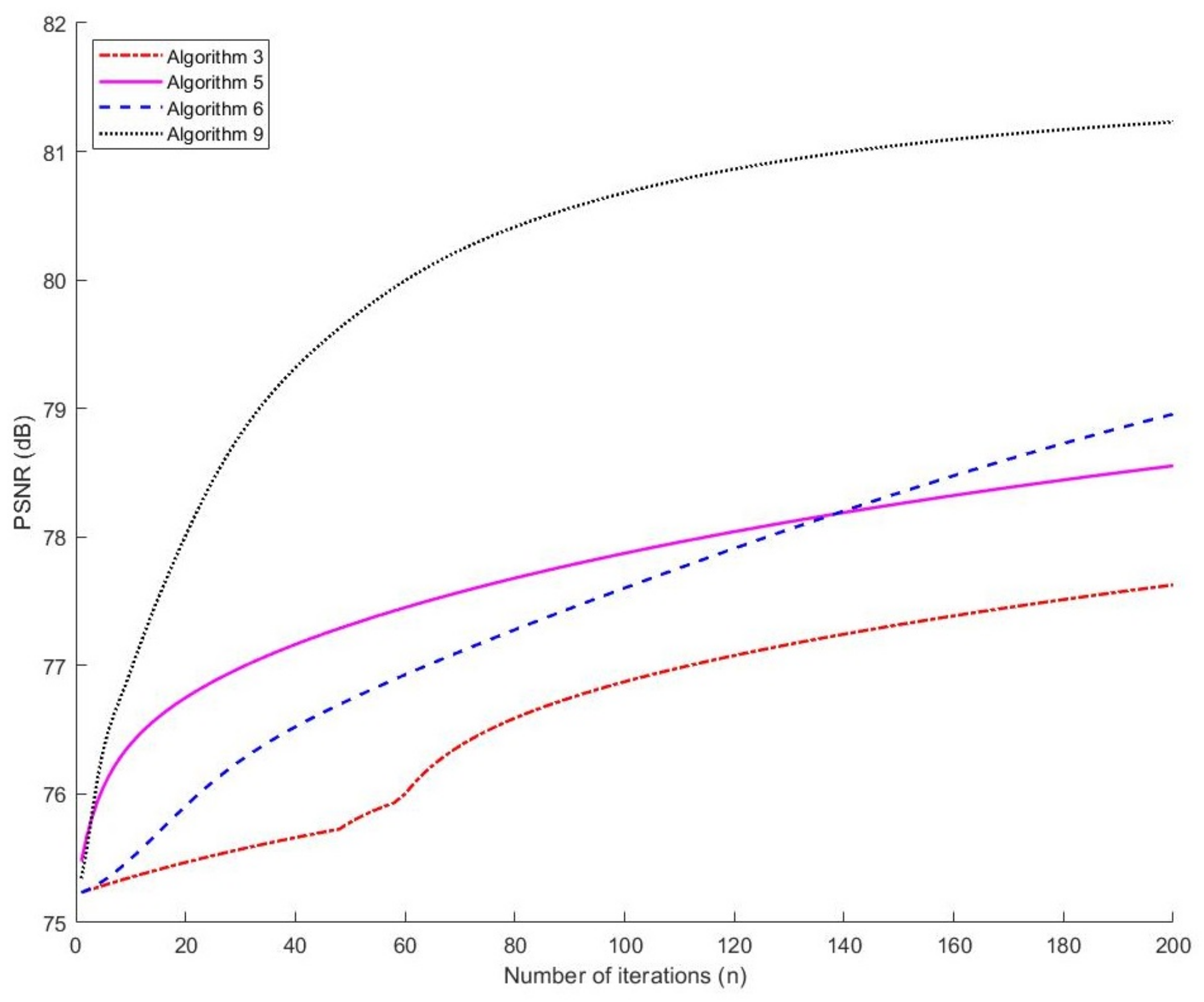
In the next experiment, we chose λ = 5 × 10 5 for each algorithm and evaluated the performance of each algorithm at the 200th iteration; see Table 5 for the results.
In Figure 4, we show the PSNR of each algorithm at each step of iteration.
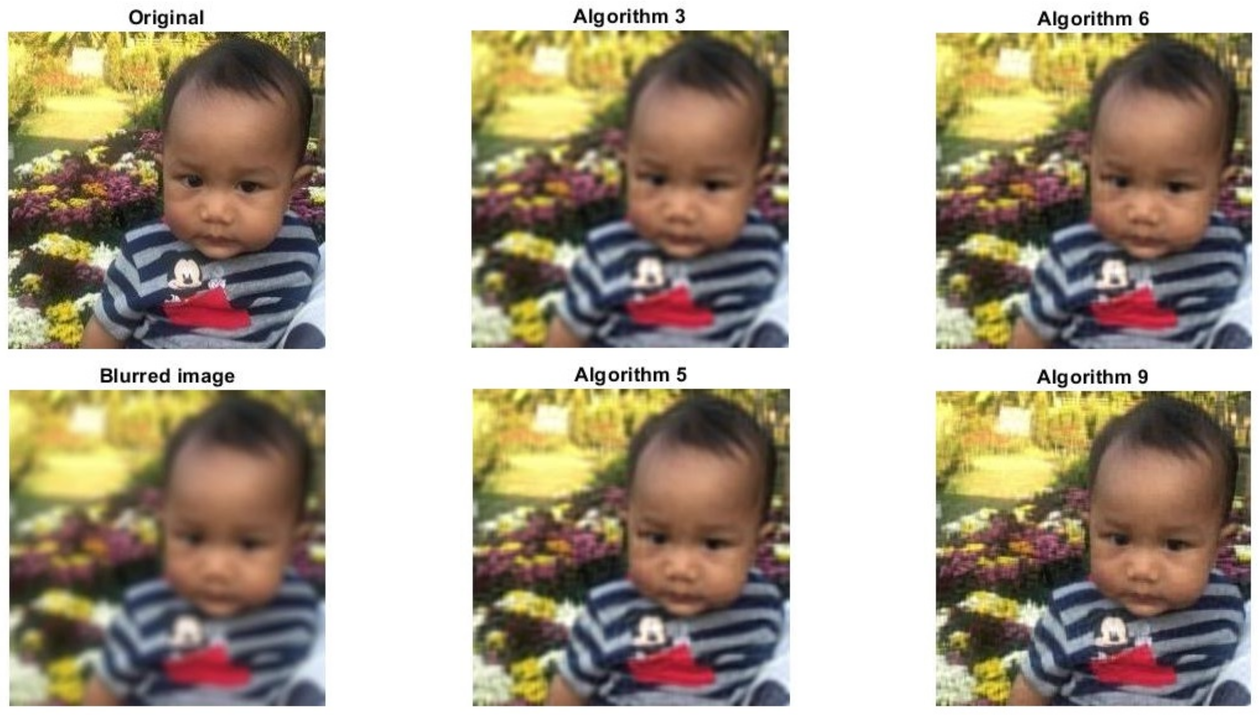
In Figure 5, we show the original test image, blurred image and deblurred images obtained from Algorithms 3, 5, 6 and 9. As we see from Table 5 and Figure 4, Algorithm 9 achieved the highest PSNR.

5. Conclusions

We introduced a new line search technique inspired by [9,19] and used this technique along with the inertial step to construct a new accelerated algorithm for solving convex minimization problems in the form of the sum of two lower semicontinuous convex functions. We proved its weak convergence to a solution of (1), which did not require an L-Lipschitz continuity of f , as well as its complexity theorem. We note that many forward–backward-type algorithms require f to be L-Lipschitz continuous in order to obtain the convergence theorem; see [10,16,18] for examples. Our proposed algorithm is easy to employ, since an L-Lipschitz constant of f does not need to be calculated. Moreover, we also utilized an inertial technique to improve the convergence behavior of our proposed algorithm. In order to show that our algorithm performed better than other line search algorithms mentioned in the literature, we conducted some experiments on classification and image restoration problems. In our experiments, we evaluated the performance of each algorithm based on selecting its suitable parameters, especially the regularization parameter. It was evidenced that our proposed algorithm performed better than the other algorithms on both data classification and image restoration problems. Moreover, we observed from [19,20] that the inertial parameter β n = t n 1 t n + 1 of FISTA and Algorithm 6 satisfied the condition sup n β n = 1 , while our algorithm required a more strict condition, n = 1 + β n < + , to ensure its convergence to a solution of (1), which was a limitation of our algorithm. We also note that the convergence of FISTA and Algorithm 6 cannot be obtained under the condition sup n β n = 1 . Therefore, it is very interesting to find a weaker condition on β n that still ensure the convergence of the algorithm to a solution of (1).

Author Contributions

Writing—original draft preparation, P.S.; software and editing, D.C.; supervision, S.S. All authors read and agreed to the published version of the manuscript.

Funding

Thailand Science Research and Innovation: IRN62W0007, Chiang Mai University.

Data Availability Statement

All data is available at https://archive.ics.uci.edu accessed on 17 May 2021.

Acknowledgments

P. Sarnmeta was supported by the Post-Doctoral Fellowship of Chiang Mai University, Thailand. This research was also supported by Chiang Mai University and Thailand Science Research and Innovation under the Project IRN62W0007.

Conflicts of Interest

The authors declare no conflict of interest.

References

  1. Kaltenbacher, B.; Rundell, W. On the identification of a nonlinear term in a reaction-diffusion equation. Inverse Probl. 2019, 35, 115007. [Google Scholar] [CrossRef] [Green Version]
  2. Kaltenbacher, B.; Rundell, W. The inverse problem of reconstructing reaction–diffusion systems. Inverse Probl. 2020, 36, 065011. [Google Scholar] [CrossRef]
  3. Averós, J.C.; Llorens, J.P.; Uribe-Kaffure, R. Numerical simulation of non-linear models of reaction-diffusion for a DGT sensor. Algorithms 2020, 13, 98. [Google Scholar] [CrossRef] [Green Version]
  4. Lukyanenko, D.; Yeleskina, T.; Prigorniy, I.; Isaev, T.; Borzunov, A.; Shishlenin, M. Inverse problem of recovering the initial condition for a nonlinear equation of the reaction-diffusion-advection type by data given on the position of a reaction front with a time delay. Mathematics 2021, 9, 342. [Google Scholar] [CrossRef]
  5. Lukyanenko, D.; Borzunov, A.; Shishlenin, M. Solving coefficient inverse problems for nonlinear singularly perturbed equations of the reaction-diffusion-advection type with data on the position of a reaction front. Commun. Nonlinear Sci. Numer. Simul. 2021, 99, 105824. [Google Scholar] [CrossRef]
  6. Egger, H.; Engl, H.W.; Klibanov, M.V. Global uniqueness and Hölder stability for recovering a nonlinear source term in a parabolic equation. Inverse Probl. 2004, 21, 271. [Google Scholar] [CrossRef]
  7. Beilina, L.; Klibanov, M.V. A Globally convergent numerical method for a coefficient inverse problem. SIAM J. Sci. Comput. 2008, 31, 478–509. [Google Scholar] [CrossRef]
  8. Klibanov, M.V.; Li, J.; Zhang, W. Convexification for an inverse parabolic problem. Inverse Probl. 2020, 36, 085008. [Google Scholar] [CrossRef]
  9. Kankam, K.; Pholasa, N.; Cholamjiak, C. On convergence and complexity of the modified forward–backward method involving new line searches for convex minimization. Math. Methods Appl. Sci. 2019, 42, 1352–1362. [Google Scholar] [CrossRef]
  10. Combettes, P.L.; Wajs, V. Signal recovery by proximal forward–backward splitting. Multiscale Model. Simul. 2005, 4, 1168–1200. [Google Scholar] [CrossRef] [Green Version]
  11. Luo, Z.Q. Applications of convex optimization in signal processing and digital communication. Math. Program. 2003, 97, 177–207. [Google Scholar] [CrossRef]
  12. Xiong, K.; Zhao, G.; Shi, G.; Wang, Y. A convex optimization algorithm for compressed sensing in a complex domain: The complex-valued split Bregman method. Sensors 2019, 19, 4540. [Google Scholar] [CrossRef] [Green Version]
  13. Chen, M.; Zhang, H.; Lin, G.; Han, Q. A new local and nonlocal total variation regularization model for image denoising. Cluster Comput. 2019, 22, 7611–7627. [Google Scholar] [CrossRef]
  14. Zhang, Y.; Li, X.; Zhao, G.; Cavalcante, C.C. Signal reconstruction of compressed sensing based on alternating direction method of multipliers. Circuits Syst. Signal Process 2020, 39, 307–323. [Google Scholar] [CrossRef]
  15. Parekh, A.; Selesnick, I.W. Convex fused lasso denoising with non-convex regularization and its use for pulse detection. In Proceedings of the 2015 IEEE Signal Processing in Medicine and Biology Symposium, Philadelphia, PA, USA, 12 December 2015; pp. 21–30. [Google Scholar]
  16. Hanjing, A.; Suantai, S. A fast image restoration algorithm based on a fixed point and optimization method. Mathematics 2020, 8, 378. [Google Scholar] [CrossRef] [Green Version]
  17. Lions, P.L.; Mercier, B. Splitting algorithms for the sum of two nonlinear operators. SIAM J. Numer. Anal. 1979, 16, 964–979. [Google Scholar] [CrossRef]
  18. Boţ, R.I.; Csetnek, E.R. An inertial forward–backward-forward primal-dual splitting algorithm for solving monotone inclusion problems. Numer. Algorithms 2016, 71, 519–540. [Google Scholar] [CrossRef] [Green Version]
  19. Beck, A.; Teboulle, M. A fast iterative shrinkage-thresholding algorithm for linear inverse problems. SIAM J. Imaging Sci. 2009, 2, 183–202. [Google Scholar] [CrossRef] [Green Version]
  20. Bello Cruz, J.Y.; Nghia, T.T. On the convergence of the forward–backward splitting method with line searches. Optim. Methods Softw. 2016, 31, 1209–1238. [Google Scholar] [CrossRef] [Green Version]
  21. Polyak, B.T. Some methods of speeding up the convergence of iteration methods. USSR Comput. Math. Math. Phys. 1964, 4, 1–17. [Google Scholar] [CrossRef]
  22. Attouch, H.; Cabot, A. Convergence rate of a relaxed inertial proximal algorithm for convex minimization. Optimization 2019, 69, 1281–1312. [Google Scholar] [CrossRef]
  23. Alvarez, F.; Attouch, H. An inertial proximal method for maxi mal monotone operators via discretiza tion of a nonlinear oscillator with damping. Set-Valued Anal. 2001, 9, 3–11. [Google Scholar] [CrossRef]
  24. Van Hieu, D. An inertial-like proximal algorithm for equilibrium problems. Math. Methods Oper. Res. 2018, 88, 399–415. [Google Scholar] [CrossRef]
  25. Chidume, C.E.; Kumam, P.; Adamu, A. A hybrid inertial algorithm for approximating solution of convex feasibility problems with applications. Fixed Point Theory Appl. 2020, 2020. [Google Scholar] [CrossRef]
  26. Burachik, R.S.; Iusem, A.N. Set-Valued Mappings and Enlargements of Monotone Operators; Springer: Berlin/Heidelberg, Germany, 2008. [Google Scholar]
  27. Takahashi, W. Introduction to Nonlinear and Convex Analysis; Yokohama Publishers: Yokohama, Japan, 2009. [Google Scholar]
  28. Moudafi, A.; Al-Shemas, E. Simultaneous iterative methods for split equality problem. Trans. Math. Program. Appl. 2013, 1, 1–11. [Google Scholar]
  29. Huang, G.B.; Zhu, Q.Y.; Siew, C.K. Extreme learning machine: Theory and applications. Neurocomputing 2006, 70, 489–501. [Google Scholar] [CrossRef]
  30. Tibshirani, R. Regression shrinkage and selection via the lasso. J. R. Stat. Soc. B Methodol. 1996, 58, 267–288. [Google Scholar] [CrossRef]
  31. Fisher, R.A. The use of multiple measurements in taxonomic problems. Ann. Eugen. 1936, 7, 179–188. [Google Scholar] [CrossRef]
  32. Detrano, R.; Janosi, A.; Steinbrunn, W.; Pfisterer, M.; Schmid, J.J.; Sandhu, S.; Guppy, K.H.; Lee, S.; Froelicher, V. International application of a new probability algorithm for the diagnosis of coronary artery disease. Am. J. Cardiol. 1989, 64, 304–310. [Google Scholar] [CrossRef]
  33. Forina, M.; Leardi, R.; Armanino, C.; Lanteri, S. PARVUS: An Extendable Package of Programs for Data Exploration; Elsevier: Amsterdam, The Netherlands, 1988. [Google Scholar]
  34. Thung, K.-H.; Raveendran, P. A Survey of Image Quality Measures. In Proceedings of the IEEE Technical Postgraduates (TECHPOS) International Conference, Kuala Lumpur, Malaysia, 14–15 December 2009; pp. 1–4. [Google Scholar]
Figure 1. PSNR of Algorithm 3 (left) and Algorithm 5 (right) with respect to λ at the 200th iteration.
Mathematics 09 01562 g001
Figure 2. PSNR of Algorithm 6 (left) and Algorithm 9 (right) with respect to λ at the 200th iteration.
Mathematics 09 01562 g002
Figure 3. A graph of the PSNR of each algorithm with respect to λ at the 200th iteration.
Mathematics 09 01562 g003
Figure 4. A graph of the PSNR of each algorithm at Iteration Number 1 to 200.
Mathematics 09 01562 g004
Figure 5. Deblurred images of each algorithm at the 200th iteration.
Mathematics 09 01562 g005
Table 1. Number of samples in each fold for all datasets.
IrisHeart DiseaseWine
TrainTestTrainTestTrainTest
Fold 1135152733016117
Fold 2135152723116018
Fold 3135152723116018
Fold 4135152723116018
Fold 5135152733016018
Fold 6135152733016018
Fold 7135152733016018
Fold 8135152733016018
Fold 9135152733016018
Fold 10135152733016117
Table 2. Chosen parameters for each algorithm.
Algorithm 3Algorithm 5Algorithm 6Algorithm 9
σ 0.490.1240.490.124
δ 0.10.10.10.1
θ 0.10.10.10.1
Table 3. Chosen λ for each algorithm.
Regularization Parameter λ
IrisHeart DiseaseWine
Algorithm 3 0.001 0.003 0.02
Algorithm 5 0.01 0.03 0.006
Algorithm 6 0.9 0.2 0.003
Algorithm 9 0.003 0.16 0.17
Table 4. Average accuracy of each algorithm at the 300th iteration with 10-fold cv.
IrisHeart DiseaseWine
TrainTestTrainTestTrainTest
Algorithm 392.3790.6781.8580.5297.5797.16
Algorithm 594.3794.0083.5381.8498.0097.19
Algorithm 696.6796.0084.4283.4999.2598.33
Algorithm 998.5298.6784.3083.8299.3899.44
Table 5. PSNR of each algorithm at the 200th iteration.
PSNR (dB)
Algorithm 377.62
Algorithm 578.55
Algorithm 678.95
Algorithm 981.29
Publisher’s Note: MDPI stays neutral with regard to jurisdictional claims in published maps and institutional affiliations.

