
Modeling COVID-19 Cases Statistically and Evaluating Their Effect on the Economy of Countries


Abstract
:1. Introduction and Review of Literature
- (i)
- (ii)
- The GHSI, where a relationship between the health impact of the COVID-19 pandemic and the ΔGDP% is expected;
- (iii)
- The country’s average risk and its standard deviation (StdDev) with this risk being measured by country default spreads (CDS), where a higher risk StdDev is expected to have a negative impact on the ΔGDP%;
- (iv)
- Belongingness of the country to the OECD group, where a positive effect on the ΔGDP% is expected if the country belongs to the OECD;
- (v)
2. Material and Methods
2.1. The Data
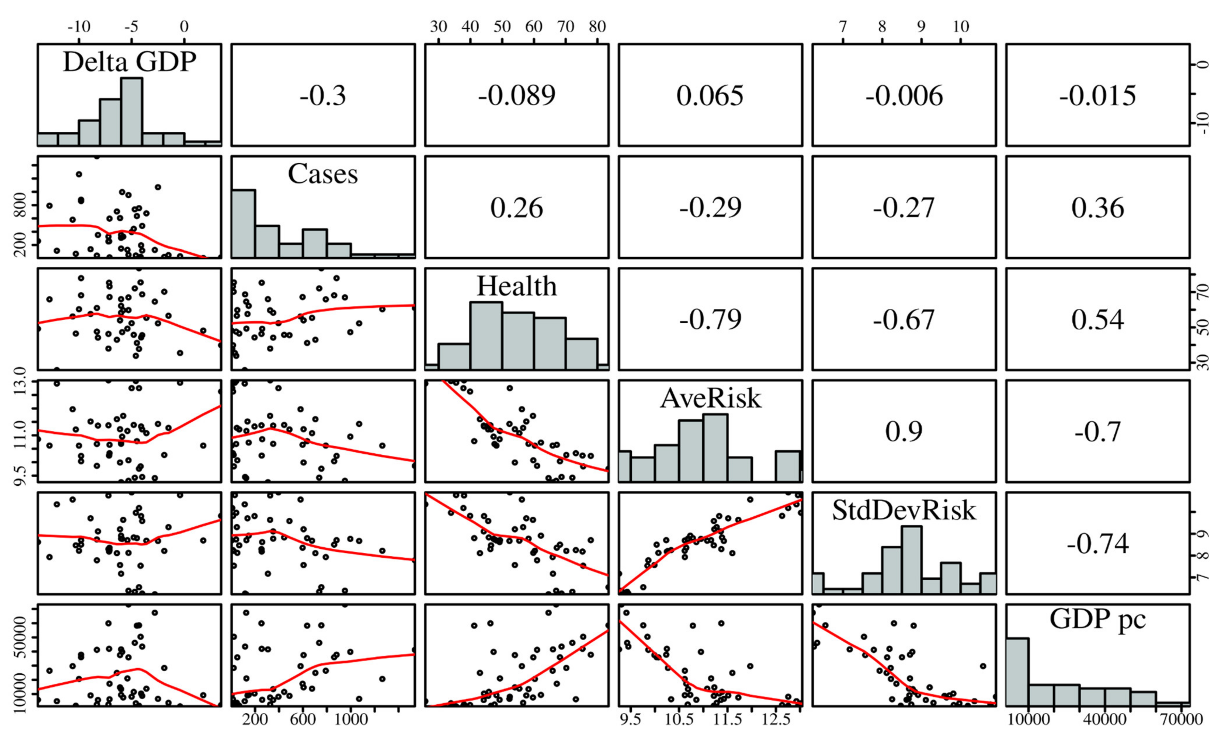
2.2. Specification of Variables and Data Exploratory Analysis
- is the ΔGDP%;
- is the value of related to the disease rate measured by the number of COVID-19 cases at the peak of the pandemic per million inhabitants from its start in March 2020 until 31 December 2020;
- is the value of associated with the GHSI for 2019;
- is the value of , the logarithm of the risk average;
- ) is the value of , the logarithm of the risk StdDev;
- is the value of , a dichotomous variable for OECD belongingness;
- is the value of , which is a control variable linked to the GDPpc;
2.3. The Statistical Models
2.4. Specification of Models
- (i)
- is the GDP variation percentage in the country i;
- (ii)
- is the number of COVID-19 cases per million inhabitants in the country i;
- (iii)
- is the GHSI in the country i;
- (iv)
- is the logarithm of the risk average measured through CDS in the country i;
- (v)
- is the logarithm of the risk standard StdDev through CDS in the country i.
- (i)
- is the GDP variation percentage in the country i;
- (ii)
- is the number of COVID-19 cases per million inhabitants in the country i;
- (iii)
- is the GHSI in the country i;
- (iv)
- is the logarithm of the risk average measured through CDS in the country i;
- (v)
- is the logarithm of the risk StdDev in the country i;
- (vi)
- is an indicator of OECD belongingness in the country i.
- (i)
- is the GDP variation percentage in the country i;
- (ii)
- is the number of COVID-19 cases per million inhabitants in the country i;
- (iii)
- is the GHSI in the country i;
- (iv)
- is the logarithm of the risk average measured through CDS in the country i;
- (v)
- is the logarithm of the risk StdDev in the country i;
- (vi)
- is an indicator of OECD belongingness in the country i;
- (vii)
- is the GDP per capita in the country i.
- (a)
- Normally distributed errors, that is, ;
- (b)
- Independency of the model errors, that is, under normality, we have , for , with as indicated below Equation (1);
- (c)
- Homogeneity or heterogeneity of variances for these errors. The homogeneity of variances assumption indicates that , for all , that is, we are only modeling the mean of because is assumed as constant (homogeneous). However, if is not constant (heterogeneous) by , we must also model it asthat is,where is the covariate associated with the country , with .
3. Results
3.1. Statistical Analysis under Homogeneity
- The COVID-19 cases per million inhabitants are significant statistically, indicating the effect that this variable has on each country’s economy in this study;
- In general, by increasing one case per million inhabitants, under the condition that all the remaining covariates remain fixed, we harm the GDP of 0.0026%, or 2.6%, per 1000 infected per million inhabitants on average;
- The results of the proposed models show an of 12.6% on average, implying a low level of regression adjustment and suggesting that another type of model specification is required for better characterization.
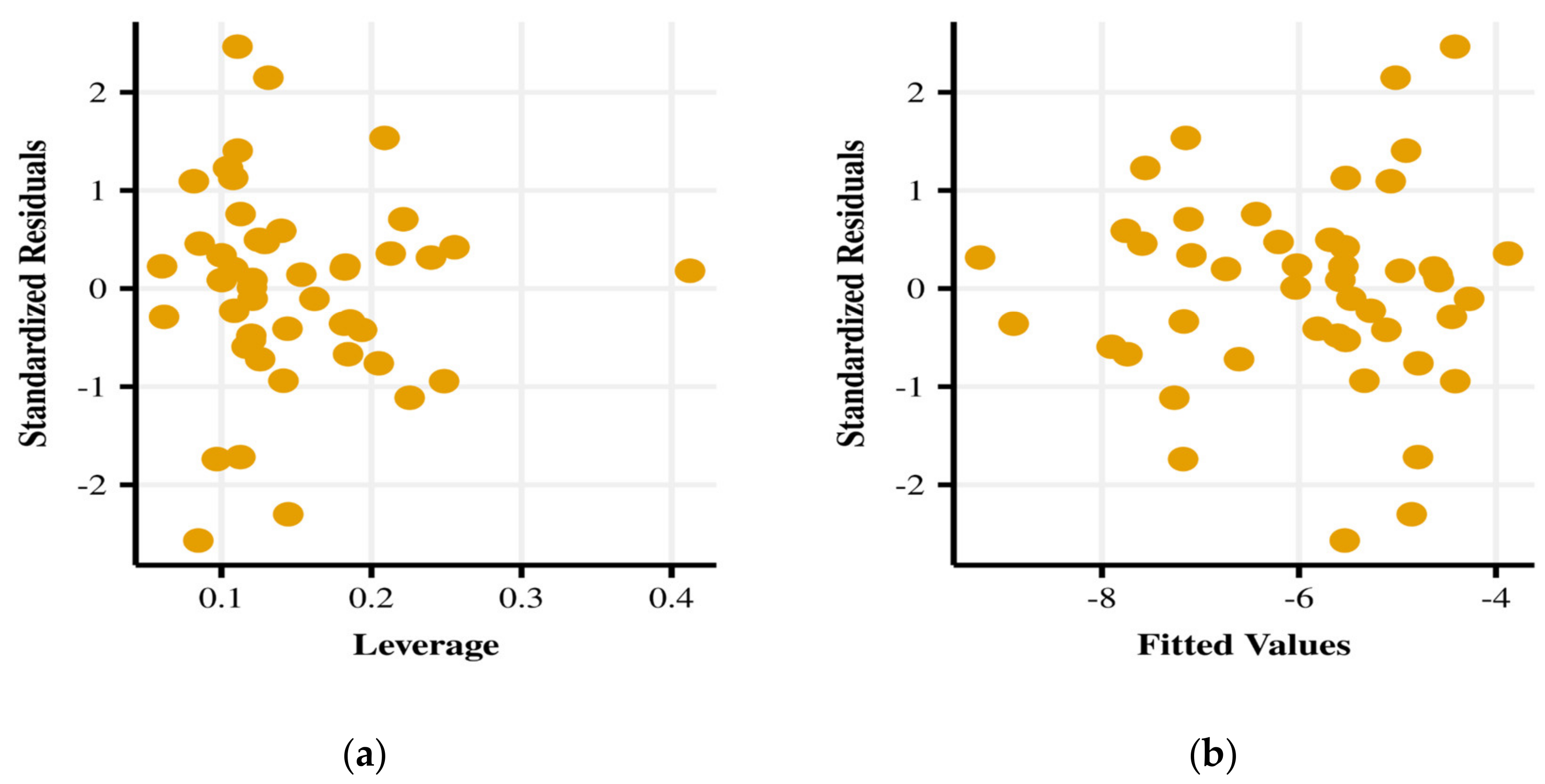
3.2. Statistical Analysis under Heterogeneity
- The null hypothesis of homoscedasticity was rejected for Models 1 and 2 at a 10% significance;
- In the case of Model 3, the homoscedasticity hypothesis was not rejected.
- Models 1 and 2 presented significant parameters for the covariates: COVID-19 cases and log(RiskStdDev);
- All models rejected the null hypothesis that the coefficients defining the variance are equal to zero, suggesting that a model does not need to remove the covariates related to the variance for its adequate specification.
- For Model 1, we detected the GDP variation percentage of the countries decreased by 0.0031 when COVID-19 cases increased by one point, under the condition that all the remaining covariates remain fixed.
- For Model 2, this increase was 0.0029, implying a 3% drop in the GDP variation percentage for each 1000 infected people per million inhabitants at the COVID-19 peak, showing a link between the health impact of the pandemic and the economic impact of the countries under study.
- OECD belongingness showed a negative effect, under the condition that all the remaining covariates remain fixed, implying that the economy of OECD countries was more strongly impacted when facing the pandemic phenomenon. However, it is not significant for our model.
- Nevertheless, countries with a higher logarithm of the risk StdDev were negatively impacted, suggesting the existence of other mechanisms affecting the economy of countries when facing problems due to the global pandemic.
- For both models, the variables that were not significant are log(RiskAve) and Health.
4. Conclusions and Future Research
Author Contributions
Funding
Institutional Review Board Statement
Informed Consent Statement
Data Availability Statement
Acknowledgments
Conflicts of Interest
References
- Huang, C.; Wang, Y.; Li, X.; Ren, L.; Zhao, J.; Hu, Y.; Zhang, L.; Fan, G.; Xu, J.; Cao, B.; et al. Clinical features of patients infected with 2019 novel coronavirus in Wuhan, China. Lancet 2020, 395, 497–506. [Google Scholar] [CrossRef] [Green Version]
- Guan, W.J.; Ni, Z.Y.; Hu, Y.; Liang, W.H.; Ou, C.Q.; He, J.X.; Liu, L.; Shan, H.; Lei, C.L.; Hui, D.S.C.; et al. Clinical Characteristics of Coronavirus Disease 2019 in China. N. Engl. J. Med. 2020, 382, 1708–1720. [Google Scholar] [CrossRef]
- Lu, R.; Zhao, X.; Li, J.; Niu, P.; Yang, B.; Wu, H.; Wang, W.; Song, H.; Huang, B.; Zhu, N.; et al. Genomic characterisation and epidemiology of 2019 novel coronavirus: Implications for virus origins and receptor binding. Lancet 2020, 395, 565–574. [Google Scholar] [CrossRef] [Green Version]
- Chan, J.F.W.; Yuan, S.; Kok, K.H.; To, K.K.W.; Chu, H.; Yang, J.; Xing, F.; Liu, J.; Yip, C.C.Y.; Poon, R.W.S.; et al. A familial cluster of pneumonia associated with the 2019 novel coronavirus indicating person-to-person transmission: A study of a family cluster. Lancet 2020, 395, 514–523. [Google Scholar] [CrossRef] [Green Version]
- WHO. Coronavirus Disease 2019 (COVID-19). Situation Report-67; World Health Organization: Geneva, Switzerland, 2019; Available online: https://www.who.int/docs/default-source/coronaviruse/situation-reports/20200327-sitrep-67-covid-19.pdf?sfvrsn=b65f68eb_4 (accessed on 6 June 2021).
- Dayong, Z.; Min, H.; Qiang, J. Financial markets under the global pandemic of COVID-19. Financ. Res. Lett. 2020, 36, 1544–6123. [Google Scholar]
- Bei, C.; Liu, S.; Liao, Y.; Tian, G.; Tian, Z. Predicting new cases of COVID-19 and the application to population sustainability analysis. Account. Financ. 2021. [Google Scholar] [CrossRef]
- Friedson, A.I.; McNichols, D.; Sabia, J.J.; Dave, D. Shelter-in-place orders and public health: Evidence from California during the COVID-19 pandemic. J. Policy Anal. Manag. 2021, 40, 258–283. [Google Scholar] [CrossRef]
- Keogh-Brown, M.R.; Wren-Lewis, S.; Edmunds, W.J.; Smith, R.D. The macroeconomic impact of pandemic influenza: Estimates from models of the United Kingdom, France, Belgium and the Netherlands. Eur. J. Health Econ. 2010, 11, 543–554. [Google Scholar] [CrossRef]
- Harjoto, M.A.; Rossi, F. Market reaction to the COVID-19 pandemic: Evidence from emerging markets. Int. J. Emerg. Mark. 2021. [Google Scholar] [CrossRef]
- Popkova, E.; DeLo, P.; Sergi, B.S. Corporate Social Responsibility amid Social Distancing During the COVID-19 Crisis: BRICS vs. OECD Countries. Res. Int. Bus. Financ. 2021, 55, 101315. [Google Scholar] [CrossRef] [PubMed]
- Sadeh, A.; Radu, C.F.; Feniser, C.; Borsa, A. Governmental intervention and its impact on crowth, economic development, and technology in OECD countries. Sustainability 2021, 13, 166. [Google Scholar] [CrossRef]
- Salisu, A.A.; Akanni, L.O. Constructing a Global Fear Index for the COVID-19 Pandemic. Emerg. Mark. Financ. Trade 2020, 56, 2310–2331. [Google Scholar] [CrossRef]
- Chahuán-Jiménez, K.; Rubilar, R.; de la Fuente-Mella, H.; Leiva, V. Breakpoint analysis for the COVID-19 pandemic and its effect on the stock markets. Entropy 2021, 23, 100. [Google Scholar] [CrossRef] [PubMed]
- Baig, A.S.; Butt, H.A.; Haroon, O.; Rizvi, S.A.R. Deaths, panic, lockdowns and US equity markets: The case of COVID-19 pandemic. Financ. Res. Lett. 2021, 38, 101701. [Google Scholar] [CrossRef] [PubMed]
- Ngo, V.M.; Nguyen, H.H. Are fear and hope of the COVID-19 pandemic responsible for the V-shaped behaviour of global financial markets? A text-mining approach. Appl. Econ. Lett. 2021, 1–11. [Google Scholar] [CrossRef]
- Costa, C.J.; Garcia-Cintado, A.C.; Marques, K. Macroeconomic policies and the pandemic-driven recession. Int. Rev. Econ. Financ. 2021, 72, 438–465. [Google Scholar] [CrossRef]
- Yousfi, M.; Ben Zaied, Y.; Ben Cheikh, N.; Ben Lahouel, B.; Bouzgarrou, H. Effects of the COVID-19 pandemic on the US stock market and uncertainty: A comparative assessment between the first and second waves. Technol. Forecast. Soc. Chang. 2021, 167, 120710. [Google Scholar] [CrossRef]
- El-Morshedy, M.; Altun, E.; Eliwa, M.S. A new statistical approach to model the counts of novel coronavirus cases. Math. Sci. 2021, 1–14. [Google Scholar] [CrossRef]
- Altig, D.; Baker, S.; Barrero, J.M.; Bloom, N.; Bunn, P.; Chen, S.; Davis, S.J.; Leather, J.; Meyer, B.; Mihaylov, E.; et al. Economic uncertainty before and during the COVID-19 pandemic. J. Public Econ. 2020, 191, 104274. [Google Scholar] [CrossRef]
- Canelli, R.; Fontana, G.; Realfonzo, R.; Passarella, M.V. Are EU Policies Effective to Tackle the Covid-19 Crisis? The Case of Italy. Rev. Political Econ. 2021, 33, 432–461. [Google Scholar] [CrossRef]
- Havrlant, D.; Darandary, A.; Muhsen, A. Early estimates of the impact of the COVID-19 pandemic on GDP: A case study of Saudi Arabia. Appl. Econ. 2021, 53, 1317–1325. [Google Scholar] [CrossRef]
- Hürtgen, P. Fiscal space in the COVID-19 pandemic. Appl. Econ. 2021, 1–16. [Google Scholar] [CrossRef]
- Jena, P.R.; Majhi, R.; Kalli, R.; Managi, S.; Majhi, B. Impact of COVID-19 on GDP of major economies: Application of the artificial neural network forecaster. Econ. Anal. Policy 2021, 69, 324–339. [Google Scholar] [CrossRef]
- Li, W.; Chien, F.; Kamran, H.W.; Aldeehani, T.M.; Sadiq, M.; Nguyen, V.C.; Taghizadeh-Hesary, F. The nexus between COVID-19 fear and stock market volatility. Econ. Res. Ekon. Istraživanja 2021, 1–22. [Google Scholar] [CrossRef]
- Marti, L.; Puertas, R. European countries’ vulnerability to COVID-19: Multicriteria decision-making techniques. Econ. Res. Ekon. Istraživanja 2021, 1–12. [Google Scholar] [CrossRef]
- Shafiullah, M.; Khalid, U.; Chaudhry, S.M. Do stock markets play a role in determining COVID-19 economic stimulus? A cross-country analysis. World Econ. 2021. [Google Scholar] [CrossRef]
- Welfens, P.J.J. Macroeconomic and health care aspects of the coronavirus epidemic: EU, US and global perspectives. Int. Econ. Econ. Policy 2020, 17, 295–362. [Google Scholar] [CrossRef]
- Kinnunen, J.; Akademi, T.A.; Georgescu, I. Bucharest University of Economics Disruptive Pandemic as a Driver towards Digital Coaching in OECD Countries. Rev. Rom. Pentru Educ. Multidimens 2020, 12, 55–61. [Google Scholar] [CrossRef]
- Wei, C.; Lee, C.C.; Hsu, T.C.; Hsu, W.T.; Chan, C.C.; Chen, S.C.; Chen, C.J. Correlation of population mortality of COVID-19 and testing coverage: A comparison among 36 OECD countries. Epidemiol. Infect. 2021, 149, e1. [Google Scholar] [CrossRef] [PubMed]
- Wildman, J. COVID-19 and income inequality in OECD countries. Eur. J. Health Econ. 2021, 22, 455–462. [Google Scholar] [CrossRef] [PubMed]
- König, M.; Winkler, A. Monitoring in real time: Cross-country evidence on the COVID-19 impact on GDP growth in the first half of 2020. COVID Econ. 2020, 57, 132–153. [Google Scholar]
- Kucukefe, B. Clustering macroeconomic impact of COVID-19 in OECD countries and China. Ekonomi Politika Ve Finans Araştırmaları Dergisi 2020, 5, 280–291. [Google Scholar]
- Pan, J.; Singleton, K.J. Default and recovery implicit in the term structure of sovereign CDS spreads. J. Financ. 2008, 63, 2345–2384. [Google Scholar] [CrossRef] [Green Version]
- Fontana, A.; Scheicher, M. An analysis of euro area sovereign CDS and their relation with government bonds. J. Bank. Financ. 2016, 62, 126–140. [Google Scholar] [CrossRef]
- Hair, J.F., Jr.; Black, W.C.; Babin, B.J.; Anderson, R.E. Multivariate Data Analysis; Pearson: Harlow, UK, 2014. [Google Scholar]
- Huerta, M.; Leiva, V.; Liu, S.; Rodriguez, M.; Villegas, D. On a partial least squares regression model for asymmetric data with a chemical application in mining. Chemom. Intell. Lab. Syst. 2019, 190, 55–68. [Google Scholar] [CrossRef]
- Velasco, H.; Laniado, H.; Toro, M.; Leiva, V.; Lio, Y. Robust Three-Step Regression Based on Comedian and Its Performance in Cell-Wise and Case-Wise Outliers. Mathematics 2020, 8, 1259. [Google Scholar] [CrossRef]
- James, G.; Witten, D.; Hastie, T.; Tibshirani, R. An Introduction to Statistical Learning; Springer: Cham, Switzerland, 2013; Volume 112, p. 18. [Google Scholar]
- Kokholm, T. Pricing and hedging of derivatives in contagious markets. J. Bank. Financ. 2016, 66, 19–34. [Google Scholar] [CrossRef]
- Oikonomikou, L.E. Modeling financial market volatility in transition markets: A multivariate case. Res. Int. Bus. Financ. 2018, 45, 307–322. [Google Scholar] [CrossRef] [Green Version]
- Lewis, V.; Roth, M. The financial market effects of the ECB’s asset purchase programs. J. Financ. Stab. 2019, 43, 40–52. [Google Scholar] [CrossRef]
- Ahundjanov, B.B.; Akhundjanov, S.B.; Okhunjanov, B.B. Information Search and Financial Markets under COVID-19. Entropy 2020, 22, 791. [Google Scholar] [CrossRef]
- Umaña-Hermosilla, B.; de la Fuente-Mella, H.; Elórtegui-Gómez, C.; Fonseca-Fuentes, M. Multinomial logistic regression to estimate and predict the perceptions of individuals and companies in the face of the COVID-19 pandemic in the Ñuble Region, Chile. Sustainability 2020, 12, 9553. [Google Scholar] [CrossRef]
- De la Fuente-Mella, H.; Vallina, A.; Solis, R. Stochastic analysis of the economic growth of OECD countries. Econ. Res. Ekon. Istraživanja 2020, 33, 2189–2202. [Google Scholar] [CrossRef] [Green Version]
- Greene, W.H. Econometric Analysis; Pearson: New York, NY, USA, 2018. [Google Scholar]
- Altonji, J.G.; Segal, L.M. Small-Sample Bias in GMM Estimation of Covariance Structures. J. Bus. Econ. Stat. 1996, 14, 353. [Google Scholar] [CrossRef] [Green Version]
- Clark, T.E. Small-sample properties of estimators of nonlinear models of covariance structure. J. Bus. Econ. Stat. 1996, 14, 367–373. [Google Scholar]
- Santos, L.; Barrios, E.B. Small Sample Estimation in Dynamic Panel Data Models: A Simulation Study. Open J. Stat. 2011, 1, 58–73. [Google Scholar] [CrossRef] [Green Version]
- Harvey, A.C. Estimating Regression Models with Multiplicative Heteroscedasticity. Econometrica 1976, 44, 461. [Google Scholar] [CrossRef]
- De la Fuente-Mella, H.; Rojas, J.L.; Leiva, V. Econometric modeling of productivity and technical efficiency in the Chilean manufacturing industry. Comput. Ind. Eng. 2020, 139, 105793. [Google Scholar] [CrossRef]
- Vallina, A.M.; de la Fuente-Mella, H.; Solis, R. International trade and innovation: Delving in Latin American commerce. Acad. ARLA 2020, 33, 535–547. [Google Scholar] [CrossRef]
- Díaz-García, J.A.; Galea, M.; Leiva, V. Influence diagnostics for multivariate elliptic regression linear models. Commun. Stat. Theory Methods 2003, 32, 625–641. [Google Scholar] [CrossRef]
- Leiva, V.; Saulo, H.; Souza, R.; Aykroyd, R.G.; Vila, R. A new BISARMA time series model for forecasting mortality using weather and particulate matter data. J. Forecast. 2021, 40, 346–364. [Google Scholar] [CrossRef]
- Sánchez, L.; Leiva, V.; Galea, M.; Saulo, H. Birnbaum-Saunders Quantile Regression Models with Application to Spatial Data. Mathematics 2020, 8, 1000. [Google Scholar] [CrossRef]
- Saulo, H.; Dasilva, A.; Leiva, V.; Sánchez, L.; de la Fuente-Mella, H. Log-symmetric quantile regression models. Stat. Neerl. 2021. [Google Scholar] [CrossRef]
- Carrasco, J.M.F.; Figueroa-Zuñiga, J.I.; Leiva, V.; Riquelme, M.; Aykroyd, R.G. An errors-in-variables model based on the Birnbaum–Saunders distribution and its diagnostics with an application to earthquake data. Stoch. Environ. Res. Risk Assess. 2020, 34, 369–380. [Google Scholar] [CrossRef]
- Liu, Y.; Mao, C.; Leiva, V.; Liu, S.; Neto, W.A.S. Asymmetric autoregressive models: Statistical aspects and a financial application under COVID-19 pandemic. J. Appl. Stat. 2021, 1–25. [Google Scholar] [CrossRef]
- Elzeki, O.M.; Shams, M.; Sarhan, S.; Elfattah, M.A.; Hassanien, A.E. COVID-19: A new deep learning computer-aided model for classification. PeerJ Comput. Sci. 2021, 7, e358. [Google Scholar] [CrossRef] [PubMed]
- Palacios, C.; Reyes-Suárez, J.; Bearzotti, L.; Leiva, V.; Marchant, C. Knowledge Discovery for Higher Education Student Retention Based on Data Mining: Machine Learning Algorithms and Case Study in Chile. Entropy 2021, 23, 485. [Google Scholar] [CrossRef] [PubMed]
- Bustos, N.; Tello, M.; Droppelmann, G.; Garcia, N.; Feijoo, F.; Leiva, V. Machine learning techniques as an efficient alternative diagnostic tool for COVID-19 cases. Signa Vitae 2021. [Google Scholar] [CrossRef]


| Year; Reference | Author(s) | Variable(s) |
|---|---|---|
| 2020; [1] | Huang, C.; Wang, Y.; Li, X.; et al. | COVID-19 cases |
| 2021; [7] | Bei, C.C.; Liu, S.P.; Liao, Y.; Tian, G.L.; Tian Z.C. | |
| 2021; [8] | Friedson, A.I.; McNichols, D.; Sabia, J.J.; Dave D. | |
| 2021; [19] | El-Morshedy, M.; Altun, E.; Eliwa, M.S. | |
| 2010; [9] | Keogh-Brown, M.R.; Wren-Lewis, S.; Edmunds, W.J.; Smith, R.D. | COVID-19 cases, economic effects |
| 2020; [20] | Altig, D.; Baker, S.; Barrero, J.M.; et al. | |
| 2020; [20] | Altig, D.; Baker, S.; Barrero, J.M.; et al. | COVID-19 cases, GDP |
| 2021; [21] | Canelli, R.; Fontana, G.; Realfonzo, R.; Passarella, M.V. | |
| 2021; [22] | Havrlant, D.; Darandary, A.; Muhsen, A. | |
| 2021; [23] | Hurtgen, P. | |
| 2021; [24] | Jena, P.R.; Majhi, R.; Kalli, R.; Managi, S.; Majhi, B. | |
| 2021; [25] | Li, W.Q.; Chien, F.S.; Kamran, H.W.; Aldeehani, T.M.; Sadiq, M.; Nguyen, V.C.; Taghizadeh-Hesary, F. | |
| 2021; [26] | Marti, L.; Puertas, R. | |
| 2021; [27] | Shafiullah, M.; Khalid, U.; Chaudhry, S.M. | |
| 2020; [28] | Welfens, P.J.J. | |
| 2021; [10] | Harjoto, M.A.; Rossi, F. | COVID-19 cases, belongingness to OECD |
| 2021; [11] | Popkova, E.; DeLo, P.; Sergi, B.S. | |
| 2021; [12] | Sadeh, A.; Radu, C.F.; Feniser, C.; Borsa, A. | |
| 2020; [28] | Welfens, P.J.J. | |
| 2020; [29] | Kinnunen, J.; Georgescu, I. | |
| 2020; [28] | Welfens, P.J.J. | COVID-19 cases, GHSI |
| Country | GDP% | Country | GDP% | Country | GDP% | Country | GDP% |
|---|---|---|---|---|---|---|---|
| Australia | −4.2 | France | −9.8 | Nigeria | −4.3 | Serbia | −2.5 |
| Belgium | −8.3 | Germany | −6.0 | Norway | −2.8 | Slovakia | −7.1 |
| Brazil | −5.8 | Hungary | −6.1 | NZ | −6.1 | SK | −1.9 |
| Bulgaria | −4.0 | Italy | −10.6 | Pakistan | −0.4 | Spain | −12.8 |
| Canada | −7.1 | India | −10.3 | Peru | −13.9 | SL | −4.6 |
| Chile | −6.0 | Indonesia | −1.5 | Philippines | −8.3 | Sweden | −4.7 |
| China | 1.8 | Irak | −12.1 | Poland | −3.6 | Switzerland | −5.3 |
| Colombia | −8.2 | Iceland | −7.2 | Portugal | −10.0 | Thailand | −7.1 |
| Croatia | −9.0 | Israel | −5.9 | Qatar | −4.5 | Turkey | −5.0 |
| Cyprus | −6.4 | Japan | −5.3 | Romania | −4.8 | Ukraine | −7.2 |
| Egypt | 3.5 | Malaysia | −6.0 | Russia | −4.1 | UK | −9.8 |
| Finland | −4.0 | Mexico | −8.9 | SA | −5.4 | US | −4.3 |
| Variable | Mean | StdDev | Minimum | Maximum |
|---|---|---|---|---|
| GDP% | −5.9 | 3.4 | −13.9 | 3.5 |
| COVID-19 cases | 410.9 | 378.4 | 3.2 | 1536.0 |
| Health | 55.4 | 13.0 | 25.8 | 83.5 |
| RiskAve | 10.9 | 1.1 | 9.3 | 13.0 |
| RiskStdDev | 8.7 | 1.2 | 6.2 | 10.9 |
| GDPpc | 23.4 | 20.3 | 1.326 | 7.3 |
| Model 1 | Model 2 | Model 3 | |
|---|---|---|---|
| Variable | GDP% | GDP% | GDP% |
| Cases | −0.00277 | −0.00248 | −0.00263 |
| (−2.29, 0.03) ** | (−2.12, 0.04) ** | (−2.17, 0.04) ** | |
| Health | −0.00916 | 0.00551 | 0.0121 |
| (−0.15, 0.88) n.s. | (0.10, 0.92) n.s. | (0.21, 0.83) n.s. | |
| log(RiskAve) | 0.900 | 0.840 | 0.876 |
| (0.65, 0.52) n.s. | (0.61, 0.54) n.s. | (0.63, 0.53) n.s. | |
| log(RiskStdDev) | −1.037 | −1.036 | −0.691 |
| (−1.24, 0.22) n.s. | (−1.27, 0.21) n.s. | (−0.74, 0.47) n.s. | |
| OECD | −0.906 | −1.430 | |
| (−0.82, 0.42) n.s. | (−1.47, 0.15) n.s. | ||
| GDPpc | 0.0000352 | ||
| (0.99, 0.33) n.s. | |||
| Constant | −5.175 | −4.985 | −9.209 |
| (−0.42, 0.67) n.s. | (−0.40, 0.69) n.s. | (−0.66, 0.51) n.s. | |
| 11.4% | 12.5% | 14.0% | |
| F-statistic | 1.360 | 1.170 | 1.080 |
| Breusch–Pagan/Cook–Weisberg Test for Heteroscedasticity | |||
| (1) | 3.46 | 5.15 | 2.08 |
| (0.063) * | (0.023) ** | (0.149) n.s. | |
| Model 1 | Model 2 | |
|---|---|---|
| Variable | GDP% | GDP% |
| Cases | −0.00312 | −0.00285 |
| (−3.56, 0.00) *** | (−3.05, 0.00) *** | |
| Health | −0.0672 | −0.0574 |
| (−1.40, 0.16) n.s. | (−1.07, 0.283) n.s. | |
| log(RiskAve) | 1.370 | 0.874 |
| (1.24, 0.22) n.s. | (0.76, 0.45) n.s. | |
| log(RiskStdDev) | −2.036 | −1.750 |
| (−2.78, 0.01) *** | (−2.23, 0.03) ** | |
| OECD | −0.827 | |
| (−0.76, 0.45) n.s. | ||
| Constant | 1.897 | 4.546 |
| (0.20, 0.84) n.s. | (0.48, 0.63) n.s. | |
| ) | ||
| Cases | −0.000828 | −0.000659 |
| (−1.14, 0.25) n.s. | (−0.69, 0.49) n.s. | |
| Health | −0.0491 | −0.00990 |
| (−1.54, 0.12) n.s. | (−0.22, 0.82) n.s. | |
| log (RiskAve) | 0.974 | 1.124 |
| (1.30, 0.19) n.s. | (1.40, 0.16) n.s. | |
| log (RiskStdDev) | −0.863 | −0.759 |
| (−1.34, 0.18) n.s. | (−0.99, 0.32) n.s. | |
| OECD | −0.814 | |
| (−1.11, 0.27) n.s. | ||
| Constant | 1.889 | −2.500 |
| (0.30, 0.76) n.s. | (−0.36, 0.72) n.s. | |
| Likelihood ratio test for | ||
| (4), (5) | 13.06 | 14.34 |
| (<0.001) *** | (<0.001) *** | |
Publisher’s Note: MDPI stays neutral with regard to jurisdictional claims in published maps and institutional affiliations. |
© 2021 by the authors. Licensee MDPI, Basel, Switzerland. This article is an open access article distributed under the terms and conditions of the Creative Commons Attribution (CC BY) license (https://creativecommons.org/licenses/by/4.0/).
Share and Cite
de la Fuente-Mella, H.; Rubilar, R.; Chahuán-Jiménez, K.; Leiva, V. Modeling COVID-19 Cases Statistically and Evaluating Their Effect on the Economy of Countries. Mathematics 2021, 9, 1558. https://doi.org/10.3390/math9131558
de la Fuente-Mella H, Rubilar R, Chahuán-Jiménez K, Leiva V. Modeling COVID-19 Cases Statistically and Evaluating Their Effect on the Economy of Countries. Mathematics. 2021; 9(13):1558. https://doi.org/10.3390/math9131558
Chicago/Turabian Stylede la Fuente-Mella, Hanns, Rolando Rubilar, Karime Chahuán-Jiménez, and Víctor Leiva. 2021. "Modeling COVID-19 Cases Statistically and Evaluating Their Effect on the Economy of Countries" Mathematics 9, no. 13: 1558. https://doi.org/10.3390/math9131558
APA Stylede la Fuente-Mella, H., Rubilar, R., Chahuán-Jiménez, K., & Leiva, V. (2021). Modeling COVID-19 Cases Statistically and Evaluating Their Effect on the Economy of Countries. Mathematics, 9(13), 1558. https://doi.org/10.3390/math9131558