Relocation Scheduling in a Two-Machine Flow Shop with Resource Recycling Operations

Abstract

This paper considers a variant of the relocation problem, which is formulated from an urban renewal project. There is a set of jobs to be processed in a two-machine flow shop subject to a given initial resource level. Each job consumes some units of the resource to start its processing on machine 1 and will return some amount of the resource when it is completed on machine 2. The amount of resource released by a job is not necessarily equal to the amount of resource acquired by the job for starting the process. Subject to the resource constraint, the problem is to find a feasible schedule whose makespan is minimum. In this paper, we first prove the NP-hardness of two special cases. Two heuristic algorithms with different processing characteristics, permutation and non-permutation, are designed to construct feasible schedules. Ant colony optimization (ACO) algorithms are also proposed to produce approximate solutions. We design and conduct computational experiments to appraise the performances of the proposed algorithms.

1. Introduction

Scheduling is a decision-making process that allocates limited resources to tasks in a given time period to optimize certain objectives in manufacturing as well as service industries [1]. Usually, resources are considered as machines that process the assigned tasks in manufacturing industries. In some scheduling contexts, there could be different extra resources, like capital, crews and technicians, storage space, energy, computer memory, and so on, that are required to support the execution of the tasks. Such scheduling problems are known as resource-constrained scheduling. Resource-constrained project scheduling problems (RCPSP) have received considerable attention for decades. Please refer to Brucker, Drexl, Möhring, Neumann, and Pesch [2], Habibi, Barzinpour, and Sadjadi [3] Herroelen, De Reyck, and Demeulemeester [4], Issa and Tu [5] for comprehensive reviews on RCPSP. The resource constraint featured in the relocation problem is different traditional ones in the sense that the amount of resource released by an activity is not necessarily the same as that acquired for commencing the activity. This study investigates the relocation problem in a two-machine flow shop with the specific feature of a resource recycling mechanism.

The construction industry have various optimization decisions to address in the project course [6,7]. The relocation problem originated from the public house redevelopment project in Boston [8,9]. The project had a set of buildings to be torn down and erected for redevelopment. During the redevelopment process, current tenants of the buildings under reconstruction needed to be relocated to temporary housing units. They could be assigned to new housing units. It was not mandatory for tenants to reside at the same place they lived before. Therefore, the authority had to determine a minimum budget of temporary housing units such that all tenants could be successfully relocated. Kaplan [8] first formulated the relocation problem of determining a feasible redevelopment sequence of the buildings with the initial budget. In the view of optimization, this problem can also be described as finding a feasible sequence of the redevelopment buildings that reflects the minimum initial budget. Kaplan and Amir [10] showed that the relocation problem is mathematically equivalent to the two-machine flow shop scheduling problem for minimizing makespan, implying that the basic relocation problem can be solved by the classical Johnson’s algorithm [11].

Lin and Huang [12] first introduced the recycling operations for yielding the resource into the study on the relocation problem. In previous studies on the relocation problem, the resource is consumed when a job starts to process and returns immediately when it is completed. However, the concept of the resource recycling is assumed that we need to have a mechanism or procedure to recycle the resource before the resource can be used for later jobs. Therefore, a job is divided into two separate parts on two dedicated machines: one processed on machine 1 and the other for recycling the resource on machine 2. The operations on machine 1 should have sufficient resource so that they can commence the processing, and the operations on machine 2 should wait for the completion of its corresponding counterpart operations jobs on machine 1. However, the job sequences on the two machines are not necessarily the same. Cheng, Lin and Huang [13] presented an integer linear program formulation for the permutation case, in which the job sequences on all machines are the same. They also investigated the non-permutation case. We continue to study this relocation problem and discuss more theoretical proofs. Then, we present heuristic algorithms and ant colony optimization (ACO) algorithms for both permutation and non-permutation sequences to find feasible schedules with resource constraints for minimum makespan.

The rest of this paper is organised as follows. In Section 2, we present problem statements and give a numerical example followed by a literature review. The complexity results of two special cases are discussed in Section 3. In Section 4 and Section 5, we present heuristic algorithms and ant colony optimization algorithms for constructing approximate schedules. Computational experiments and performance statics of the algorithms are given in Section 6. We conclude this search and suggest research directions for future study in Section 7.

2. Problem Definition

In this section, we first introduce the notation that will be used throughout our research. Then, a formal problem formulation follows. An integer programming model is also proposed. The notations are listed below:

Notation:
$\mathcal{N}=\{1,2,\dots n\}$	set of jobs to be processed;
p1,j	processing time of job j on machine 1;
p2,j	processing time of job j on machine 2;
αj	resource requirement of job j;
𝛽j	amount of the resource returned by job j;
$\sigma =({\sigma }_1,{\sigma }_2,\dots {\sigma }_n)$	a particular sequence of the jobs
	(assumed for the case of permutation schedules);
v0	initial resource level;
vt	resource level at time t ≥ 0;
Cm,j	completion time of job j on machine m, m = 1, 2.

We formally state the problem as follows: From time zero onwards, a set of jobs $\mathcal{N}=\{1,2,\dots ,n\}$ is available to be processed in a two-stage flow shop consisting of machine 1 and machine 2. Initially, the common resource pool contains $v_0$ units of a single type of resource. Job $j\in \mathcal{N}$ can start processing only if machine 1 is not occupied and the resource level is larger than or equal to ${\alpha }_j$. When job j starts processing, it immediately consumes ${\alpha }_j$ units of the resource and takes $p_{1j}$ units of time on machine 1. After the operation on machine 1 is completed, $p_{2j}$ units of time are required to complete its resource recycling operation on machine 2. When job j completes on machine 2, it produces and returns ${\beta }_j$ units of the resource back to the resource pool. No preemption on either machine is permitted. Note that there is no strict relation between ${\alpha }_j$ and ${\beta }_j$. That is, ${\beta }_j$ could be smaller than, equal to, or larger than ${\alpha }_j$. The goal is to minimize the makespan. In other words, we want to find a feasible schedule that completes all jobs in the shortest time.

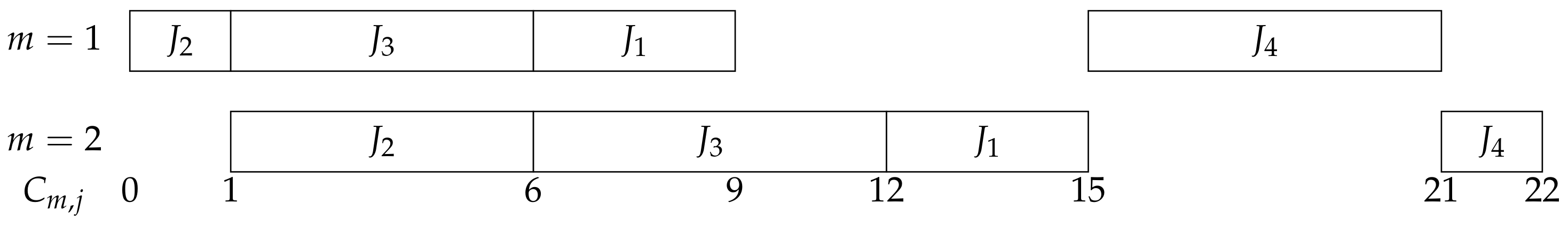
To illustrate the problem definition, we consider an instance of four jobs with an initial resource level $v_0=6$. The parameters are shown below in Table 1. We construct two example schedules.

Table 1. An example of four jobs.

	${\mathit{p}}_{1,\mathit{j}}$	${\mathit{p}}_{2,\mathit{j}}$	${\mathit{\alpha }}_{\mathit{j}}$	${\mathit{\beta }}_{\mathit{j}}$
job 1	3	3	8	9
job 2	1	5	3	10
job 3	5	6	3	8
job 4	6	1	11	4

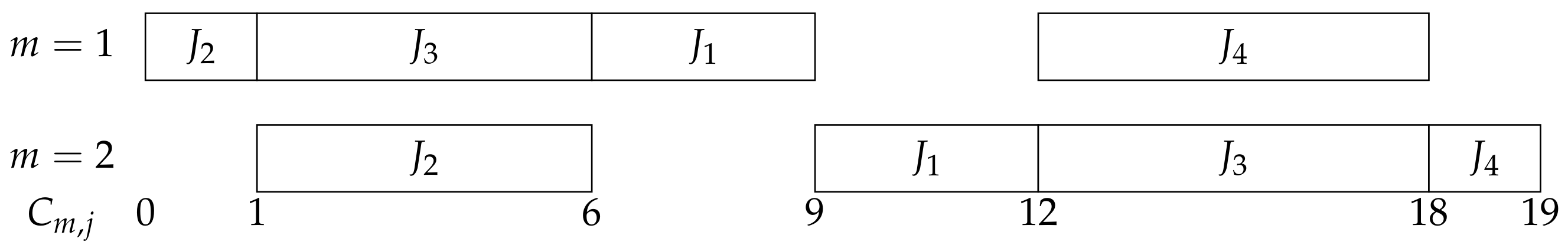
Figure 1 shows an optimal permutation solution with $C_{max}$ = 22, and Figure 2 shows an optimal non-permutation solution with $C_{max}$ = 19. Both of them are feasible. In this example, it is clear that the non-permutation solution can attain a better makespan than the permutation one.

Figure 1. Permutation solution.

Figure 2. Non-permutation solution.

Literature Review

To describe our problem, we denote use the standard three-field notation $F2\left|rp\right|C_{max}$, proposed by Graham et al. [14]. The first field indicates the machine environment of a two-machine flow shop, where the first machine is the operation of the building being torn down and the second machine is about re-constructing buildings corresponding to resource recycling operations. The second field indicates that the specific conditions for the job characteristics, i.e., the relocation problem. The last field specifies the objective function of makespan.

The study on the relocation problem was inaugurated by Kaplan [8] in 1986. The fundamental purpose of the basic relocation problem is to minimize the initial budget required for guaranteeing project feasibility. In Kaplan’s study, multiple working crews were considered that if resources were sufficient, i.e., a number of buildings could be simultaneously developed. Kaplan and Amir [10] formulated the application of relocation problem as an integer program. They also noted the relationship between the minimum budget in relocation feasibility and the minimum makespan of two-machine flow shop scheduling, which is solvable in $O(nlogn)$ time [11]. To reflect real situations of the housing redevelopment project in East Boston, Kaplan, and Berman [15] refined the integer programming model and scheduling heuristics. Applications like the financial constraints on single machine scheduling problems [16] which can be reduced to the two-machine flow shop scheduling problem as a special case of the relocation problem. The relocation problem is also related to the memory management issue in database system in practical term [17]. Amir and Kaplan [17] showed that minimizing the makespan on parallel machines is NP-hard. Kononov and Lin [18] proved that parallel-machine setting is strongly NP-hard even if there are only two working crews and all jobs have the same processing time. They also designed approximation algorithms with performance ratio analysis for two special cases.

Cheng and Lin [19] presented more proofs and proposed the concept of composite jobs that can reduce the computational time for handling the relocation problem. Cheng and Lin [20] also demonstrated the concept of relocation scheduling to give an economic interpretation of Johnson’s algorithm. The concept can also simplify proofs and reduce time complexity in some two-machine flow shop scheduling problems. There are other extensions from the relocation problem. Lin and Tseng [21] considered the problem with processing times and deadline constraints. Furthermore, they provided a complexity result and two polynomial algorithms to solve the restricted problems. Lin and Tseng [22] proposed a branch-and-bound algorithm to maximize the resource level under a specified due date and considered the precedence constraints [23] that is NP-hard even if the precedence constraints are specified by a bi-partite graph. Lin and Cheng [24] showed two relocation problems of minimizing the maximum tardiness is strongly NP-hard and of minimizing the number of tardy jobs under a due date is NP-hard even when all the jobs have an equal tardy weight and resource requirement. Based on the generalized due dates proposed by Hall [25], Lin and Liu [26] extended the scheduling problem and designed a branch-and-bound algorithm to reduce the computational time required. Sevastyanov, Lin and Huang [27] considered the relocation problem with arbitrary release dates. They developed a multi-parametric dynamic programming algorithm to solve the case with a fixed number if distinct due release dates and analyzed complexity of different problem settings. Kononov and Lin [28] considered minimizing the total weighted completion time and proved four special cases are strong NP-hardness. They established the equivalence between the UET (unit-execution-time) case and the unit-weighted case and presented a 2-approximation algorithm for the restricted special cases.

As per the feature of resource recycling in the relocation problem, there are some existing works. Lin and Huang [12] first introduced the concept of resource recycling. This operation can be processed on a secondary recycling machine that the whole procession can be described as a two-machine flow shop scheduling problem. In this paper, they showed that it is NP-hard and designed three heuristic algorithms to compose approximate schedules. Problem formulation and some complexity results were discussed in Cheng, Lin and Huang [13]. They presented integer linear programming models for finding the feasible permutation sequence and non-permutation sequence with minimum makespan. Lin [29] considered the setting where processing and recycling are carried out on the same single machine. The problem is a generalization of the knapsack problem. He designed a pseudo-polynomial time dynamic programming algorithm and formulated an integer program to solve this recycling problem that operations are processed on the same single machine.

3. Complexity Analysis

This section is dedicated to discussion of the complexity results of the problem of several special cases. First, let instance $\mathcal{I}$ contain n jobs with $p_{1,j}$, $p_{2,j}$, ${\alpha }_j$, and ${\beta }_j$ given for each job j and an initial resource level $v_0$. We create another instance $\overline{\mathcal{I}}$ having n jobs with ${\overline{p}}_{1,j}=p_{2,j},{\overline{p}}_{2,j}=p_{1,j},{\overline{\alpha }}_j={\beta }_j,and{\overline{\beta }}_j={\alpha }_j$ that is symmetric to the instance $\mathcal{I}$. Set the initial resource level ${\overline{v}}_0=v_0-{\sum }_{j=1}^{4q+1}({\beta }_j-{\alpha }_j)$. We claim that the two instances have the optimal makespan. The concept follows the results of Kononov and Lin [28].

Theorem 1.

(Mirror Property) Instance $\mathcal{I}$ and instance $\overline{\mathcal{I}}$ have the optimal makespan.

Proof. 

Let $\sigma =\left(\sigma \right(1),\sigma (2),\dots ,\sigma (n\left)\right)$ be a feasible permutation of jobs in the given instance $\mathcal{I}$ case. We show that $\overline{\sigma }=(\sigma \left(n\right),\sigma (n-1),\dots ,\sigma \left(1\right))$ is feasible for $\overline{\mathcal{I}}$ we created in the above. Assume ${\overline{V}}_k$ is the resource level after the jobs $\sigma \left(n\right),\dots ,\sigma (k+1)$ in $\overline{\sigma }$ complete. We have ${\overline{V}}_k-{\overline{\alpha }}_{\sigma \left(k\right)}={\overline{v}}_0+{\sum }_{j=k+1}^n({\overline{\beta }}_{\sigma \left(j\right)}-{\overline{\alpha }}_{\sigma \left(j\right)})-{\overline{\alpha }}_{\sigma \left(k\right)}=v_0+{\sum }_{j=1}^k({\beta }_{\sigma \left(j\right)}-{\alpha }_{\sigma \left(j\right)})-{\beta }_{\sigma \left(k\right)}=v_0+{\sum }_{j=1}^{k-1}({\beta }_{\sigma \left(j\right)}-{\alpha }_{\sigma \left(j\right)})-{\alpha }_{\sigma \left(k\right)}\ge 0$. The last inequality is feasible with the schedule $\sigma$. Therefore, we can get ${\overline{V}}_k\ge {\overline{\alpha }}_{\sigma \left(k\right)}$, which shows the schedule $\overline{\sigma }$ is feasible. As we know the schedule $\overline{\sigma }$ and $\sigma$ are two-stage flow shop, if their sequences are reversed, they have same processing time. Therefore, we can construct another optimal schedule if we get an optimal one.    □

For n jobs, there are $(n!)$ possible sequences when the permutation schedules are considered. If we consider the non-permutation variant, the number of schedules will become $O(n!\times n!)$ because the permutations on the two machines could be different. For technical constraints or dispatching fairness, say first comes first served, the processing sequence could be given and fixed [30,31]. In view of implementations, if an optimal schedule can be efficiently obtained from a given job sequence on either machine, we can then reduce the decision tree size from $O(n!\times n!)$ to $O(n!)$. This section will explore the complexity status of the setting with a fixed job sequence.

First, we prove the problems that when the sequence of the jobs on machine 2 is given and fixed, finding the optimal schedule is strongly NP-hard, even if all jobs have the same processing time on machine 2. On the other hand, if the given and fixed sequence of the jobs is on machine 1, we can get the same result that finding optimal schedules is also strongly NP-hard. The proof is given in the following:

3-Partition: Given an integer B and a set A of $3q$ elements $\{1,2,\dots ,3q\}$, each $j\in A$ has a size $x_j$, $B/4<x_j<B/2$, such that ${\sum }_{j=1}^{3q}{x}_j=qB$, is there a partition $A_1,A_2,\dots ,A_q$ of the set A such that ${\sum }_{x_j\in A_l}{x}_j=B$, $1\le l\le q$?

Theorem 2.

If a sequence of the jobs on machine 2 is given and fixed, then finding an optimal schedule is strongly NP-hard, even if all jobs have the same processing time on machine 2.

Proof. 

Given an instance of 3-Partition, we create a corresponding set of $4q+1$ jobs as follows:

• Enforcer jobs: $p_{1,j}=0,p_{2,j}=B,{\alpha }_j=2B,and{\beta }_j=3B,1\le j\le q;$
• Ordinary jobs: $p_{1,j}=x_i,p_{2,j}=B,{\alpha }_j=x_i,and{\beta }_j=0,q+1\le j\le 4q;$
• Final job: $p_{1,j}=3qB,p_{2,j}=B,{\alpha }_j=0,and{\beta }_j=0,j=4q+1$.

The the initial resource level $v_0=3B$. The jobs on machine 2 are sequenced in increasing order of their indices. We claim that there is a 3-Partition if there is a feasible schedule whose makespan is no greater than $(4q+1)B$.

Assume that there exists a desired partition $A_1,A_2,\dots ,A_q$ of 3-Partition. Because the total actual processing length on machine 2 is $(4q+1)B$, we know that no idle time on machine 2 is permitted. Then, we schedule the enforcer job 1 on machine one first followed by the the ordinary jobs corresponding to the three elements of $A_1$ and the resource level is brought back to $3B$. Repeat the dispatching pattern and then schedule the last job. It is to see that the schedule is feasible and the makespan is exactly $(4q+1)B$.

Assume that there is a feasible schedule whose makespan is no larger than $(4q+1)B$. The total actual processing length on machine 2 of all jobs is $(4q+1)B$. There is no idle time on machine 2. On the other hand, the total actual processing length on machine 1 is $4qB$. Considering the subsequent operations on machine 2, no idle time is allowed on machine 1. In other words, machine 1 and machine 2 cannot have any idle time in order to attain the makespan $(4q+1)B$. As given, machine 2 processes the enforcer jobs $1,2,\dots ,q$ as in their indices. Since all enforcer jobs have the same parameter values, without loss of generality we assume that the enforcer jobs also follow the same processing order on machine 1.

We first note that job 1 should start first on machine 1 for otherwise non-zero idle time will be incurred on machine 2. After completing job 1 on machine 1, the resource level drops from $3B$ to B. To start the next enforcer job 2, machine 1 wait for the previous enforcer job 1 to be completed to accumulate sufficient resources. To avoid the idle time between the first and second enforcer jobs on machine 1, we assign ordinary jobs to fill up the idle period. Let $A_1$ be the set of elements defining these ordinary jobs. If ${\sum }_{x_j\in A_1}{x}_j<B$, then there is an idle time before job 2 on machine 1. On the other hand, if ${\sum }_{x_j\in A_1}{x}_j>B$, then the resource is insufficient and the completion time of some ordinary jobs are later than the second enforcer job, leading to the idle time on machine two. As the result, ${\sum }_{x_j\in A_1}{x}_j=B$ must hold. Continuing this process, we can find subsets $A_2,\dots ,A_n$ with ${\sum }_{x_j\in A_l}{x}_j=B$, $2\le l\le q$, satisfied for the 3-Partition problem. 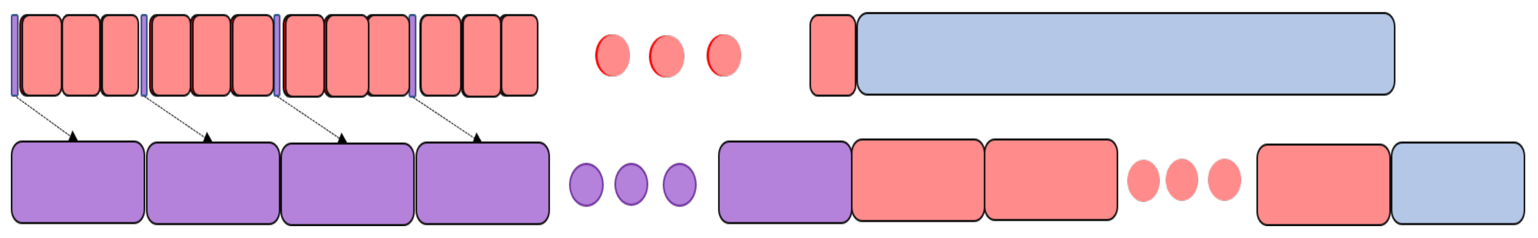Figure 3 shows the sequence of the optimal schedule: the purple blocks are enforcer jobs, the red ones are ordinary jobs, and the blue ones are final job.    □

Figure 3. Given and fixed sequence on machine 2.

Theorems 1 and 2 together imply the following result.

Theorem 3.

If a sequence of the jobs on machine 1 is given and fixed, then finding an optimal schedule is strongly NP-hard, even if all jobs have the same processing time on machine 2.

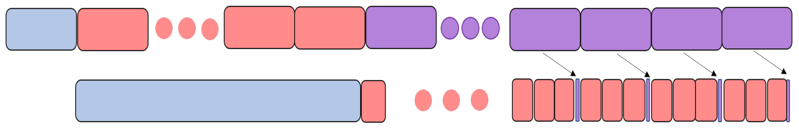
Proof. 

Owing to Theorems 1 and 2, we can get the feasibility of a given and fixed sequence of the jobs on machine 1 whose optimal schedule is strongly NP-hard. On the other hand, the idle time before job 1 on machine 2 is inevitable and the total actual processing length is $(4q+1)B$. Furthermore, the sequence of Theorem 2 whose jobs on machine 2 is given and fixed, if we reverse this two-stage flow shop sequence, we can get the given and fixed sequence of the jobs on machine 1 which is equivalent to Theorem 3. It can seen that Figure 4 is derived form Figure 3 by reversing the Gantt chart from the right. As a result, the sequences of Theorem 2 and Theorem 3 have same total processing time. Then, we get the optimal schedule.    □

Figure 4. Given and fixed sequence on machine 1.

Theorem 4.

If sequences of the jobs on machine 1 and machine 2 are given and fixed, then the optimal schedule can be found in polynomial time.

Proof. 

Assume that there is a feasible schedule whose sequences of the jobs on machine 1 and machine 2 are given and fixed. We schedule the first job on machine 1 followed by the first job on machine 2. If the resource of second job on machine 1 is insufficient, it should wait for previous job which on machine 2 to return the resource. Otherwise, it can be processed immediately when the previous job finished. Then, the job on machine 2 starts when the job on machine 1 completed. Continuing this process, we can schedule all the jobs and the makespan is minimum. On the other hand, if the job on machine 2 return resource is not enough for the next job to be processed, we can know that this sequence is not feasible. As a result, we can get an optimal schedule if sequences of the jobs on machine 1 and machine 2 are given and fixed.    □

To simplify the problem, we consider the special case where processing sequences on both machines are given. By problem definition, the two sequences are not necessarily the same. For simplicity in presentation, we re-index the jobs to follow the natural sequence ${\pi }_1=({\pi }_{1,1},{\pi }_{1,2},\dots ,{\pi }_{1,n})$ on machine 1. Let ${\pi }_2=({\pi }_{2,1},{\pi }_{2,2},\dots ,{\pi }_{2,n})$ denote the sequence on machine 2 and $v\left(t\right)$ the resource level at a specific time point t. Notations $t_1$ and $t_2$ represent the current time points on machines 1 and 2. Note that if an operation whichever finished on machine 1 or machine 2 and another operation starts on next machine simultaneously at time t, we define $v\left(t\right)$ as the resource level after the finished operation on one machine and before the starting operation on the other machine. We will use this method, outlined in Algorithm 1, to calculate makespan for the problem.

Algorithm 1: Two Sequences

In Algorithm 1, the first job of the sequence on machine 1 is processed first and there should be sufficient resource for it to start. Therefore, the first time point $t_{1,1}$ is the processing time of job 1 on machine 1, which is also $t_1$, and $v\left(t_1\right)$ is the resource level when job 1 finishes. In Line 6 we check the resource if we can process the job i on machine 1 or not. If resource is insufficient for job i on machine 1, we execute Line 11 to Line 19 for processing some job j on machine 2 to collect more resource. In Line 12, we need to check if job ${\pi }_{1,j}$ is scheduled first on machine 1 or not. Because we start to process jobs on machine 2 when the resource is not enough for machine 1, there may be several candidate jobs that can be processed on machine 2. Therefore, sometimes, $t_2$ is less than $t_1$ when the resource level is sufficient for the next job. In Lines 16 to 17, if $t_2$ is larger than $t_1$, we need to set $t_1$ equal to $t_2$, i.e., the next job on machine 1 should wait for the job on machine 2 to recycle its resource. When all the jobs on machine 1 finish, there are still some jobs on machine 2 not yet processed. As a result, we process the remaining jobs on machine 2 in the While loop of Line 20 to Line 22.

4. Heuristic Algorithms

Since the $F2\left|rp\right|C_{max}$ problem is computationally hard, it is hard to find optimal solutions when the problem size is large. We therefore design heuristic algorithms to produce approximate solutions in an acceptable time.

4.1. Permutation

We design two heuristic algorithms, using different sequences to construct feasible schedules for $F2\left|rp\right|C_{max}$ problem. If the job of the sequence does not violate the resource constraint, it must satisfy two conditions that the current resource level is sufficient for it, and that after its processing the resource level is sufficient for all remaining jobs. We denote the job sequence as $\sigma$ and the remaining jobs sequenced by Johnson’s rule using resource parameters $\alpha$ and $\beta$ as ${\sigma }_{JR}$. Recall that $v_0$ is the initial resource requirement using Johnson’s rule, and $V_{needed}$ denotes the minimum resource requirement for the remaining jobs that the sequence is the same as ${\sigma }_{JR}$ excluding job j. If the job violates the constraints, we will remove it. Then, we can get a set of feasible jobs which are the candidates to be processed next. Algorithm 2 examines each of the remaining jobs to determine if they are feasible candidates for the next position.

Algorithm 2: Check Resource

The first heuristic algorithm, JR-time Permutation Heuristic, is outlined in Algorithm 3. We define ${\sigma }_{time}$ as the remaining jobs sequenced by Johnson’s rule using $p_{1,i}$ and $p_{2,i}$ and ${\sigma }_{JR}$ using ${\alpha }_i$ and ${\beta }_i$. Before a job is processed, we need to run CheckResource function for checking whether the job can be processed or not. Then, we append the job to the partial schedule $\sigma$. Repeat the same step until all the jobs are processed.

Algorithm 3: JR-time Permutation Heuristic

The second heuristic, JR-resource Permutation Heuristic, is the same as the previous one except that the job sequence is ordered by Johnson’s rule using ${\alpha }_i$ and ${\beta }_i$.

4.2. Non-Permutation

We design two heuristic algorithms that construct non-permutation schedules for $F2\left|rp\right|C_{max}$. Let ${\sigma }_1$ be the sequence of the jobs processed on machine 1, and ${\sigma }_2$ the job sequence on machine 2. Let $\widehat{{\sigma }_2}$ contain the jobs eligible for processing on machine 2. Algorithm 4 processes the jobs on machine 1 first. If a job satisfies the two constraints, it will be appended to the schedule. Since we want to construct a non-permutation schedule, we create $\widehat{{\sigma }_2}$ to collect the jobs which are finished on machine 1 but not yet on machine 2. When the resource level is insufficient for the candidate job, we need to process the jobs on machine 2 for acquiring more resource. Therefore, we choose the job that has the largest $\beta$ in $\widehat{{\sigma }_2}$ to be processed first. However, this strategy may lead to an idle time when we only process the selected job. To avoid this situation, we first find the arrival time of the selected job that can be processed and we call it $LargeBetaArrivalTime$ here. Then, check if the completion time of any other job is earlier than $LargeBetaArrivalTime$. Furthermore, we change the $fraction$ such that $1-fraction$ is the acceptable time range that exceeds $LargeBetaArrivalTime$.

In Line 14, if the acceptable completion time is earlier than $LargeBetaArrivalTime$, then it is appended to ${\sigma }_2$ and removed form $\widehat{{\sigma }_2}$. This process iterates until all the jobs of $\widehat{{\sigma }_2}$ are checked. After that, the job having the largest $\beta$ is appended to ${\sigma }_2$ and removed form $\widehat{{\sigma }_2}$. We repeat the above steps until all the jobs be processed and then we get a feasible non-permutation schedule.

The second heuristic, JR-time Non-Permutation Heuristic, is similar to the first one except for using $p_{1,i}$ and $p_{2,i}$ to arrange the job sequence.

Algorithm 4: JR-resource Non-Permutation Heuristic

5. Ant Colony Optimization

In this section, we design an ACO algorithm to solve our problem. We will explain the framework and strategies of the algorithm for producing the approximate sequence.

State transition rule: In the ACO search process, each ant selects the next node to visit by calculating the preference for each path according to the pheromone intensity and heuristic visibility. In the proposed ACO algorithm, the preference $P_{ij}$ of an ant, positioned at node i, for selecting node j is defined as:

$$P_{ij}=\left\{\begin{array}{cc}\frac{{\tau }_{ij}^{w_{\tau }}{\eta }_{ij}^{w_{\eta }}}{{\sum }_{j\in I}{\tau }_{ij}^{w_{\tau }}{\eta }_{ij}^{w_{\eta }}},\hfill & \mathrm{if}\mathrm{j}\in \mathit{I};\hfill \\ 0,\hfill & \mathrm{otherwise},\hfill \end{array}\right.$$

(1)

where ${\tau }_{ij}$ is the pheromone intensity on the link from node i to node j, and ${\eta }_{ij}$ the visibility value from node i to node j, and I the set of remaining admissible jobs to be processed. Parameters $w_{\tau }$ and $w_{\eta }$ control the relative importance of ${\tau }_{ij}$ and ${\eta }_{ij}$. The greater a parameter is, the more influence of it to the preference value. In our design, the visibility value ${\eta }_{ij}$ is based on a greedy strategy. We prefer less processing times on both machines, less resource requirement, and larger amount of the resource returned by job for priority selection. Visibility value is defined as:

$${\eta }_{ij}=\frac{{\beta }_j}{{\alpha }_j+p_{1j}+p_{2j}}.$$

(2)

We use preference values $P_{ij}$ for our exploration strategy. This method is just like the roulette wheel that every node, i.e., every job has their transition probability, based on which we select the next job randomly. Every node has a chance to be selected, even the probability is low.

Pheromone updating rule: After all the jobs are processed, we update the pheromone tails so that the ants can select their future paths according to previous experience. The trail intensity on link $(i,j)$ is updated as below:

$${\tau }_{ij}=(1-\rho )\times {\tau }_{ij}+\Delta {\tau }_{ij},$$

(3)

where $\rho$ represents the pheromone evaporation rate, and $\Delta {\tau }_{ij}$ the incremental pheromone between nodes i and j given as:

$$\Delta {\tau }_{ij}=\left\{\begin{array}{cc}\frac{Q}{C_k},\hfill & \mathrm{if}\mathrm{j}\in \mathrm{I};\hfill \\ 0,\hfill & \mathrm{otherwise}.\hfill \end{array}\right.$$

(4)

In the above definition, Q is an adjustable parameter and $C_k$ the completion time of the last job on machine 2. This strategy is based on policy that the less $C_k$ is, the more pheromone on the path enhanced.

Stopping criterion: The proposed ACO algorithm assigns a colony of ants to probe their own sequences and set a maximum number of iterations. When all the ants complete their routes in one iteration, we select the minimum makespan, i.e., the elite, to be our current best solution. Then, we iterate the process until reaching the maximum number of iterations. If there is a better solution in iterations, this new solution will replace the current best one.

Permutation: To take into account the resource constraints on two machines, we only choose the job that would return the sufficient resource for the remaining jobs to be successfully processed. Therefore, we use the function CheckResource before ants select the next job and then enter the ACO algorithm to get the permutation sequence. This method is similar to JR Permutation Heuristic except that we use ACO to choose the job sequence.

Non-Permutation: For non-permutation sequences, we divide the algorithm into two parts. In the first part, we use the ACO algorithm to obtain the sequence on machine 1, similar as in Permutation. In second part, the difference form Permutation is when the resource is insufficient for the next job, we use the same method $LargeBetaArrivalTime$ in JR-resource Non-Permutation Heuristic to select jobs to process on machine 2. Then, we can get a complete sequence and we use it to update the ACO algorithm. As a result, we can get the non-permutation sequence by ACO combined with the heuristic method on machine 2.

6. Computational Experiments

In this section, we present computational experiments on the proposed methods through test data to compare and analyze the performance of these algorithms. The programs were coded in Python and executed on a personal computer with an Intel(R) Core(TM) i7-8700K CPU running at 3.70 GHz with 32.0 GB RAM. The operating system is Windows 10. We will describe how the test data sets were generated. Then, we present the related parameter settings and discuss the experimental results.

Data generation schemes: In our experiments, all parameters are integer. Processing times $p_{1,j}$ and $p_{2,j}$ of jobs on different machines were generated from the uniform distribution, $[1,10]$. Resource parameters ${\alpha }_j$ and ${\beta }_j$ were generated from the uniform distribution $[1,20]$. The initial resource level was considered based on 1.1 and 1.4 times the minimum resource requirement that is at least how much the resource is needed for all the jobs of each data set. Test data sets are categorized into 8 different job numbers $n\in \{10,20,30,\dots ,80\}$. For each job number, 5 independent sets were generated. Each set also has different uniform distributions for processing times $p_{1,j}$ and $p_{2,j}$, the resource parameters ${\alpha }_j$ and ${\beta }_j$, and the initial resource requirement. That means that we have 40 different data sets in all. On each data set, say 10 jobs, heuristic algorithms were run only once since they are deterministic. For a specific setting, the values were averaged over 5 independent sets of the same setting. The ACO algorithm, due to its randomness nature, was exercised 5 runs on each data set to get its average performance.

6.1. Results of Heuristic Algorithms

In this experiment, we apply the four heuristic algorithms on different data sets. We compare permutation solutions with non-permutation ones in two different methods, namely JR-resource and JR-time. The initial resource level in all experiment results set by multiplying the minimum resource requirement by 1.1. For each problem size, the average objective value of derived solution (minimum makespan) are reported. Since the elapsed execution times of four heuristic algorithms are almost negligible, we do not show the execution time in the following tables. All detail experiment results of different data sets are shown in Appendix A.

In Table 2, the makespan of permutation sequence of perm and non-permutation is max$\beta$. It can be seen that the JR-resource algorithm can get better makespan than the JR-time algorithm. Since the constraint is considered by resource, it is obviously that when the jobs sequenced by processing time, the resource would insufficient and the jobs should wait for the resource returned which lead to idle time. In most of the data sets, the makespans of permutation heuristics are less than non-permutation ones (max$\beta$ in Table 2). However, sometimes, non-permutation can get a better solution that reported in JR-resource with 10 jobs. We speculate that some jobs on machine 2 can fill up the idle time and thus decrease the waiting time on machine 1.

Table 2. JR-resource and JR-time heuristics.

	JR-Resource		JR-Time
#	perm	max$\mathit{\beta }$	perm	max$\mathit{\beta }$
	${\mathit{C}}_{max}$
10	80	78	87	92
20	137	142	166	177
30	199	202	251	256
40	258	262	332	345
50	307	308	425	439
60	351	357	474	494
70	426	431	596	605
80	467	472	636	642

In the experiment, there are different fractions of the bearable exceeding time, which is the acceptable time length that exceeds $LargeBetaArrivalTime$, used in JR-resource and JR-time Non-Permutation Heuristics. The fraction ranges from $5/10$ to $10/10$. Table 3 is for JR-time Non-Permutation Heuristics focused on processing times, and Table 4 for the heuristics focused on ${\alpha }_i$ and ${\beta }_i$. If we do not consider the bearable exceeding time, the makespan would be more than others that bear the exceed time because there is longer idle time in the sequences. It is clear that with the 10/10 fraction we get a longer makespan. In most cases, the makespan is the same regardless of the fraction. However, sometimes it is shown that if we bear too much exceeded time, we may get worse makespan with a 5/10 fraction of 20 jobs in JR-time and 5/10 to 6/10 fractions of 10 jobs in JR-resource. The results of fractions are not better than permutation ones, so we do not have further test for different fractions with 1.4 times the initial resource level.

Table 3. Different fractions in JR-time Non-Permutation Heuristics.

	Fraction of Exceeding Time
#	10/10	9/10	8/10	7/10	6/10	5/10
	${\mathit{C}}_{max}$
10	92	88	87	87	86	86
20	177	169	166	166	166	167
30	256	252	252	252	252	252
40	345	332	332	333	333	332
50	439	424	424	425	425	425
60	494	475	475	475	475	475
70	605	595	597	597	597	597
80	642	638	638	637	637	637

Table 4. Different fraction in JR-resource Non-Permutation Heuristics.

	Fraction of Exceeding Time
#	10/10	9/10	8/10	7/10	6/10	5/10
	${\mathit{C}}_{max}$
10	78	78	78	79	80	80
20	142	138	137	137	137	137
30	202	199	199	199	199	199
40	262	258	258	258	258	258
50	308	307	307	307	307	307
60	357	351	351	351	351	351
70	431	428	426	426	426	426
80	472	467	467	467	467	467

6.2. Results of ACO Algorithms

We discuss the results of ACO algorithms with permutation and non-permutation options. We tuned several parameter values in preliminary tests to determine the setting for further experiments. We observed differences in the results, although not significant. The parameter values leading to better results were adopted as the base setting for the final computational tests. We set the two parameters $w_{\tau }=2$ and $w_{\eta }=3$ that could get better makespan in the experiment we tested before. The pheromone evaporation $\rho$ is 0.95 to avoid early convergence. Parameter Q is defined as the number of jobs divided by 10 and multiplied by 50. Setting 100 epochs for a solution with the colony size the same as the number of jobs. Then, we have each data set run this process 5 times to get an average makespan and an average elapsed execution time. The time unit here is second and “-” means that no feasible solution was found. All complete experiment results are shown in Appendix A.

In Table 5, perm indicates the permutation method, and max$\beta$ the non-permutation method presented in Section 5. M2-enum is also non-permutation sequence that is different from the method we used in max$\beta$. The difference between them is that when the resource is insufficient on machine 1, M2-enum will enumerate all the possible sequences of candidate jobs on machine 2 to find the minimum makespan and return resource. This procedure is time-consuming because the number of possible sequences we need to compare is a factorial of the number of candidate jobs on machine 2. Therefore, when the job number is larger than 30, we cannot get a solution in 3600 s. We also experiment on the integer programming method (IP) proposed by Cheng et al. [13] to solve the problem. The IP can get the optimal solutions for data sets. However, when the number of jobs is over 10, it cannot find any feasible solution in 3600 s for most data sets. Therefore, it is regarded as no solution found. With the initial resource is multiplied by 1.1, it is clear that perm can obtain a better makespan and the required run time of perm is also less than max$\beta$.

Table 5. Results of ACO algorithms and IP with 1.1 × initial resource levels.

#	perm		max$\mathit{\beta }$		M2-enum		IP
	${\mathit{C}}_{max}$	Time	${\mathit{C}}_{max}$	Time	${\mathit{C}}_{max}$	Time	${\mathit{C}}_{max}$	Time
10	69	0.41	70	0.80	69	0.84	68	446.81
20	125	2.33	128	4.54	123	27.47	-	-
30	184	8.24	187	13.46	184	3396.50	-	-
40	239	22.09	242	36.99	-	-	-	-
50	299	50.15	300	73.62	-	-	-	-
60	339	97.24	344	139.03	-	-	-	-
70	416	172.08	418	236.40	-	-	-	-
80	456	279.78	459	352.56	-	-	-	-

Table 6 indicates that with more initial resource a better makespan can be achieved, as comapred with those in Table 5. Similarly, M2-enum and IP cannot get any solution when job numbers are over 30 and 10, respectively, in 3600 s. It is also shown that when the initial resource level is larger, for like 30 jobs, M2-enum will waste more time so that it cannot find better solutions in 3600 s (Displayed in Table A18). Then, the permutation method can find an approximate solution with less time. However, results of 1.1 and 1.4 times are within spitting distance when the quantity of jobs increases. It is reckoned that the processing times of the subsequent jobs on machine 2 are larger and the resource is sufficient for them, so their starting times are later than their completion times on machine 1 and they keep processing continuous without idle time. Therefore, the makespan of larger data sets are not quite different when the initial resource increases.

Table 6. Results of ACO algorithms and IP with 1.4 × initial resource levels.

#	perm		max$\mathit{\beta }$		M2-enum		IP
	${\mathit{C}}_{max}$	Time	${\mathit{C}}_{max}$	Time	${\mathit{C}}_{max}$	Time	${\mathit{C}}_{max}$	Time
10	66	0.42	67	0.79	69	0.84	65	187.72
20	125	2.44	127	4.44	124	470.49	-	-
30	183	8.31	185	13.95	184	2967.66	-	-
40	239	21.59	241	34.04	-	-	-	-
50	299	49.88	300	69.53	-	-	-	-
60	339	95.94	343	129.10	-	-	-	-
70	416	160.34	418	226.25	-	-	-	-
80	456	263.11	458	364.20	-	-	-	-

Table 7 shows that different fractions of the bearable exceeding time used in ACO Non-Permutation algorithms with different times of the initial resource. In most cases, it would get less makespan with considering the bearable exceeding time. The makespan resulted from fractions between 5/10 and 9/10 are not quite different. It is clearly shown that the makespan of 10/10 fraction is longer than others. As a result, setting the bearable exceeding time can achieve a better performance.

Table 7. Results of different fraction in max$\beta$ of ACO with different initial resource levels.

	Fraction of Exceeding Time with 1.1 × Initial Resource Levels
#	5/10		6/10		7/10		8/10		9/10		10/10
	${\mathit{C}}_{max}$	Time	${\mathit{C}}_{max}$	Time	${\mathit{C}}_{max}$	Time	${\mathit{C}}_{max}$	Time	${\mathit{C}}_{max}$	Time	${\mathit{C}}_{max}$	Time
10	69	0.84	69	0.82	69	0.79	69	0.78	70	0.87	70	0.80
20	125	4.65	125	4.61	125	4.81	125	4.35	125	4.71	128	4.54
30	184	14.50	184	15.61	184	15.32	184	13.70	184	14.42	187	13.46
40	239	35.49	239	41.70	239	40.46	239	33.73	239	36.92	242	36.99
50	299	71.12	299	76.58	299	78.63	299	72.06	299	77.92	300	73.62
60	339	128.90	339	141.33	339	144.98	339	133.39	340	139.73	344	139.03
70	416	262.69	417	255.90	417	243.21	416	235.66	416	218.79	418	236.40
80	456	347.84	456	368.73	456	354.50	456	395.34	456	358.64	459	352.56
	Fraction of Exceeding Time with 1.4 × Initial Resource Levels
#	5/10		6/10		7/10		8/10		9/10		10/10
	${\mathit{C}}_{max}$	Time	${\mathit{C}}_{max}$	Time	${\mathit{C}}_{max}$	Time	${\mathit{C}}_{max}$	Time	${\mathit{C}}_{max}$	Time	${\mathit{C}}_{max}$	Time
10	66	0.77	66	0.78	66	0.79	66	0.82	66	0.79	67	0.79
20	125	4.52	124	4.51	124	4.56	125	4.49	124	4.54	127	4.44
30	183	13.99	183	13.85	183	13.80	183	13.98	183	13.94	185	13.95
40	239	33.55	239	33.85	239	33.83	239	34.28	239	34.18	241	34.04
50	299	70.50	298	75.06	299	71.54	299	69.69	299	70.03	300	69.53
60	339	132.19	339	130.84	339	130.32	339	130.71	340	129.45	343	129.10
70	417	214.20	416	209.34	417	242.51	416	230.94	417	224.80	418	226.25
80	456	359.57	456	359.48	456	369.24	456	379.99	456	359.53	458	364.20

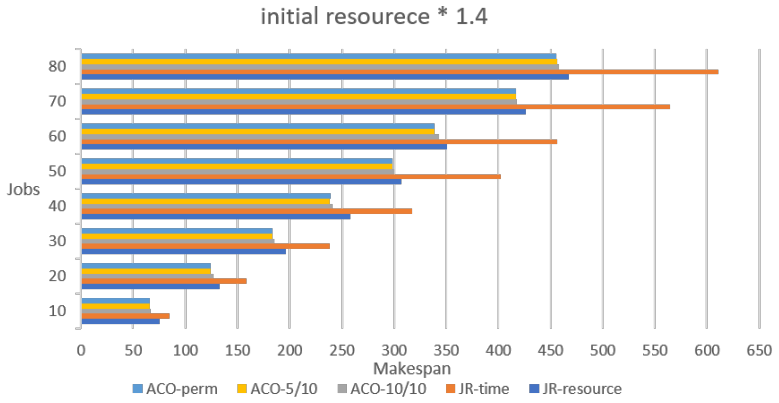
6.3. Comparison between Heuristics and ACO Algorithms

We discuss the experiment results of the heuristic and the ACO algorithms with special focus on permutation results of JR-time and JR-resource because the makespan of permutation cases are less than other non-permutation heuristic algorithms. ACO-10/10 is the 10/10 fraction of exceeding time bearable in the non-permutation ACO algorithm. We also choose the 5/10 fraction (ACO-5/10) and the permutaion of ACO (ACO-perm) as the control groups.

In Figure 5 and Figure 6, both heuristic algorithms produced larger makespan no matter if the initial resource is multiplied by 1.1 or 1.4, especially for the JR-time. However, there is still some deviations in the ACO algorithms owing to the randomness nature. Except for the above situation, 1.4 times are still better than 1.1 times in most cases with permutation and non-permutation methods, especially JR-time. We reckon that with a higher initial resource level, more jobs on machine 1 can keep continuous processing, thus reducing the idle time waiting for resource return. Concerning the ACO algorithm, it is clear that that the 5/10 fraction is better than the 10/10 case.

Figure 5. Bar chart of comparison with 1.1 × initial resource levels.

Figure 6. Bar chart of comparison with 1.4 × initial resource levels.

7. Conclusions and Future Works

In this paper, we considered the relocation problem in a two-machine flow shop scheduling problem with the second machine introduced for recycling the resource returned by jobs completed on the first machine. For this problem, we proved that given a sequence of jobs on whichever machine, the problem is still strongly NP-hard. The case with two fixed sequences of jobs on both machines can be solved in polynomial time. For the computationally hard problem, we proposed two heuristic algorithms to construct feasible schedules with permutation and non-permutation sequences. ACO algorithms were designed to find processing sequences on the two machines. Computational experiments indicates that JR-resource produced better makespan than JR-time, and both of their permutation algorithms are better than the non-permutation ones. This result is similar as in ACO algorithm that the makespan of permutation solutions are better. However, when we considered the bearable exceeding time, non-permutation sequences can get better solutions. Between heuristics and ACO algorithms, it is shown that ACO algorithms yielded schedules with less makespan.

For further studies, there is room for further improvements of our proposed solution methods by developing effective methods to arrange the job sequence on machine 2 to mitigate the incurred idle time. Furthermore, we can also combine processing time and resources as a control factor in the heuristic algorithms. It would be also interesting to deploy machine learning and reinforcement learning approaches for finding better parameter settings and updating strategies. We also note that to optimally solve the problem is still limited to small-scale instances. For larger instances, we need tighter lower bounds to facilitate the development of exact methods and provide a tight comparison base for approximation methods. Another direction is identifying application contexts in which the unique type of resource constraints, the amount of consumed resource and the amount of returned resource could be different, is applicable.

References

1. Pinedo, M. Scheduling; Springer: New York, NY, USA, 2016; Volume 29. [Google Scholar]
2. Brucker, P.; Drexl, A.; Möhring, R.; Neumann, K.; Pesch, E. Resource-constrained project scheduling: Notation, classification, models, and methods. Eur. J. Oper. Res. 1999, 112, 3–41. [Google Scholar] [CrossRef]
3. Habibi, F.; Barzinpour, F.; Sadjadi, S. Resource-constrained project scheduling problem: Review of past and recent developments. J. Proj. Manag. 2018, 3, 55–88. [Google Scholar] [CrossRef]
4. Herroelen, W.; Reyck, B.D.; Demeulemeester, E. Resource-constrained project scheduling: A survey of recent developments. Comput. Oper. Res. 1998, 25, 279–302. [Google Scholar] [CrossRef]
5. Issa, S.; Tu, Y. A survey in the resource-constrained project and multi-project scheduling problems. J. Proj. Manag. 2020, 5, 117–138. [Google Scholar] [CrossRef]
6. Ibadov, N.; Kulejewski, J.; Krzemiński, M. Fuzzy ordering of the factors affecting the implementation of construction projects in Poland. AIP Conf. Proc. 2013, 1558, 1298–1301. [Google Scholar]
7. Krzemiński, M. KASS v. 2.2. scheduling software for construction with optimization criteria description. Acta Phys. Pol. A 2016, 130, 1439–1442. [Google Scholar] [CrossRef]
8. Kaplan, E.H. Relocation models for public housing redevelopment programs. Environ. Plan. B Plan. Des. 1986, 13, 5–19. [Google Scholar] [CrossRef]
9. PHRG. New Lives for Old Buildings: Revitalizing Public Housing Project; Public Housing Group, Department of Urban Studies and Planning, MIT: Cambridge, MA, USA, 1986. [Google Scholar]
10. Kaplan, E.H.; Amir, A. A fast feasibility test for relocation problems. Eur. J. Oper. Res. 1988, 35, 201–206. [Google Scholar] [CrossRef]
11. Johnson, S.M. Optimal two- and three-stage production schedules with setup times included. Nav. Res. Logist. Q. 1954, 1, 61–68. [Google Scholar] [CrossRef]
12. Lin, B.M.T.; Huang, H.L. On the relocation problem with a second working crew for resource recycling. Int. J. Syst. Sci. 2006, 37, 27–34. [Google Scholar] [CrossRef]
13. Cheng, T.C.E.; Lin, B.M.T.; Huang, H.L. Resource-constrained flowshop scheduling with separate resource recycling operations. Comput. Oper. Res. 2012, 39, 1206–1212. [Google Scholar] [CrossRef]
14. Graham, R.L.; Lawler, E.L.; Lenstra, J.K.; Kan, A.R. Optimization and approximation in deterministic sequencing and scheduling: A survey. Ann. Discret. Math. 1979, 5, 287–326. [Google Scholar]
15. Kaplan, E.H.; Berman, O. OR hits the heights: Relocation planning at the orient heights housing project. Interfaces 1988, 18, 14–22. [Google Scholar] [CrossRef]
16. Xie, J. Polynomial algorithms for single machine scheduling problems with financial constraints. Oper. Res. Lett. 1997, 21, 39–42. [Google Scholar] [CrossRef]
17. Amir, A.; Kaplan, E.H. Relocation problems are hard. Int. J. Comput. Math. 1988, 25, 101–110. [Google Scholar] [CrossRef]
18. Kononov, A.V.; Lin, B.M.T. On relocation problems with multiple identical working crews. Discret. Optim. 2006, 3, 366–381. [Google Scholar] [CrossRef] [Green Version]
19. Cheng, T.C.E.; Lin, B.M.T. Johnson’s rule, composite jobs and the relocation problem. Eur. J. Oper. Res. 2009, 192, 1008–1013. [Google Scholar] [CrossRef] [Green Version]
20. Cheng, T.C.E.; Lin, B.M.T. Demonstrating Johnson’s algorithm via resource-constrained scheduling. Int. J. Prod. Res. 2017, 55, 3326–3330. [Google Scholar] [CrossRef]
21. Lin, B.M.T.; Tseng, S.S. Some results of the relocation problems with processing times and deadlines. Int. J. Comput. Math. 1991, 40, 1–15. [Google Scholar] [CrossRef]
22. Lin, B.M.T.; Tseng, S.S. Relocation problems of maximizing new capacities under a common due date. Int. J. Syst. Sci. 1992, 23, 1433–1448. [Google Scholar] [CrossRef]
23. Lin, B.M.T.; Tseng, S.S. Resource-requirement minimization in relocation problems with precedence constraints. In Proceedings of the ICCI `92: Fourth International Conference on Computing and Information, Toronto, ON, Canada, 28–30 May 1992; pp. 26–29. [Google Scholar]
24. Lin, B.M.T.; Cheng, T.C.E. Minimizing the weighted number of tardy jobs and maximum tardiness in relocation problem. Eur. J. Oper. Res. 1999, 116, 183–193. [Google Scholar] [CrossRef]
25. Hall, N.G. Scheduling problems with generalized due dates. IIE Trans. 1986, 18, 220–222. [Google Scholar] [CrossRef]
26. Lin, B.M.T.; Liu, S.T. Maximizing the reward in relocation problems with generalized due dates. Int. J. Prod. Econ. 2008, 115, 55–63. [Google Scholar] [CrossRef]
27. Sevastyanov, S.V.; Lin, B.M.T.; Huang, H.-L. Tight complexity analysis of the relocation problem with arbitrary release dates. Theor. Comput. Sci. 2011, 412, 4536–4544. [Google Scholar] [CrossRef] [Green Version]
28. Kononov, A.V.; Lin, B.M.T. Minimizing the total weighted completion time in the relocation problem. J. Sched. 2010, 13, 123–129. [Google Scholar] [CrossRef]
29. Lin, B.M.T. Resource-constrained scheduling with optional recycling operations. Comput. Ind. Eng. 2015, 90, 39–45. [Google Scholar] [CrossRef]
30. Shafransky, Y.M.; Strusevich, V.A. The open shop scheduling problem with a given sequence of jobs on one machine. Nav. Res. Logist. 1998, 45, 705–773. [Google Scholar] [CrossRef]
31. Lin, B.M.T.; Hwang, F.J.; Kononov, A.V. Relocation scheduling subject to fixed processing sequences. J. Sched. 2016, 19, 153–163. [Google Scholar] [CrossRef]