Computing Open Locating-Dominating Number of Some Rotationally-Symmetric Graphs

Abstract

Location detection is studied for many scenarios, such as pointing out the flaws in multiprocessors, invaders in buildings and facilities, and utilizing wireless sensor networks for monitoring environmental processes. The system or structure can be illustrated as a graph in each of these applications. Sensors strategically placed at a subset of vertices can determine and identify irregularities within the network. The open locating-dominating set S of a graph $G=(V,E)$ is the set of vertices that dominates G, and for any $i,j\in$ V(G) $N\left(i\right)\cap S\ne N\left(j\right)\cap S$ is satisfied. The set S is called the OLD-set of G. The cardinality of the set S is called open locating-dominating number and denoted by ${\gamma }^{old}\left(G\right)$. In this paper, we computed exact values of the prism and prism-related graphs, and also the exact values of convex polytopes of ${\mathcal{R}}_n$ and ${\mathcal{H}}_n$. The upper bound is determined for other classes of convex polytopes. The graphs considered here are well-known from the literature.

1. Introduction and Preliminaries

For an undirected graph $G=(V_G,E_G)$, and for any vertex $u\in V_G$, the open and closed neighborhoods are written as $N\left(u\right)$ and $N\left[u\right]$. The open locating-dominating set S of G is the set of vertices that dominates G, and for any vertices, say $w,x\in V_G$ such that $N\left(w\right)\cap S\ne N\left(x\right)\cap S$ is satisfied. The set S will be denoted as an OLD-set and the least number of elements in such a set will be denoted as ${\gamma }^{old}\left(G\right)$.

Location detection problems have been considered for several applications, including detecting faults in multiprocessors, contaminants in standard utilities, invaders in buildings and amenities, and environmental monitoring employing wireless sensor networks. The system or framework can be modeled as a graph in each of these applications. Sensors strategically placed at a subset of vertices can determine and identify irregularities in the network. Such sensors can be expensive, and therefore, it is vital to reduce the size of the OLD-set. If the detector can distinguish an invader at $N\left(u\right)$, without the ability of detecting at u, then we consider an open locating-dominating set, as studied in [1,2,3,4,5]. If a detection device can resolve an intruder in the closed neighborhood of N[u] but cannot locate the location, then we are interested in the identifying code, as studied in [6]. The identifying code I is a vertex subset of $V_G$ which dominates G, and for any $u,v\in V_G$, the relation $N\left[u\right]\cup S\ne N\left[v\right]\cup S$ holds.

The following result obtained by [7,8] presents the lower bound for the open locating-dominating number.

Theorem 1

([7,8]). Let G be a graph of order n and maximum degree $\Delta \left(G\right)$. If G has an OLD-set, then ${\gamma }^{old}\left(G\right)$ obeys

$${\gamma }^{old}\left(G\right)\ge \frac{2n}{\Delta +1}.$$

This paper continues the study of domination parameters in different rotationally-symmetric graphs. The binary locating-dominating number denoted as ${\gamma }_{l-d}^t\left(G\right)$, which is also known as the locating-dominating number, was studied in [9,10] among different classes of convex polytopes. The open locating-dominating number ${\gamma }^{old}\left(G\right)$ was studied in [11]. In this paper, motivated by these results, we study the OLD-set with minimum cardinality and ${\gamma }^{old}\left(G\right)$ values. The graphs considered in this paper are already known from the literature, and they are rotationally-symmetric. The paper is organized as follows. In Section 2, we give an improved result for the OLD-set with minimum cardinality and ${\gamma }^{old}\left(G\right)$ values for cycle graphs. The result is later employed to determine the upper bounds. In Section 3, the exact values are calculated for the prism graph ${\mathcal{D}}_n$ and the prism-related graph ${\mathcal{D}}_n^{*}$. Moreover, in Section 4, the exact values are presented for the graphs of convex polytopes ${\mathcal{R}}_n$, and ${\mathcal{H}}_n$. Section 5 comprises the upper bounds for the classes of convex polytopes ${\mathcal{S}}_n$, ${\mathcal{R}}_n^{\prime }$, ${\mathcal{A}}_n$, ${\mathcal{Q}}_n$, ${\mathcal{U}}_n$, and the web graph ${\mathbb{W}}_n$, respectively. Section 6 provides the conclusions.

2. Main Results

Cycle Graphs

The graphs considered in this paper are generated from cycle graphs. So, we provide an improved result for the open locating-dominating number of cycle graphs. The cycle graphs are 2-regular graphs. Mathematically, the vertex set is

$$\begin{array}{c}\hfill V\left(C_n\right)=\{e_p\mid p=0,\dots ,n-1\}.\end{array}$$

The edge set is

$$\begin{array}{c}\hfill E\left(C_n\right)=\{(e_p,e_{p+1})\mid p=0,\dots ,n-2\}\bigcup \{e_{n-1},e_0\}.\end{array}$$

Lemma 1.

For $n\ge 6$, we have

$${\gamma }^{old}(C_n\le \left\{\begin{array}{cc}⌈\frac{2n}{3}⌉,\hfill & n\equiv 0,2(mod3);\hfill \\ ⌈\frac{2n}{3}⌉+1\hfill & n\equiv 1(mod3).\hfill \end{array}\right.$$

Proof. 

To show the upper bound, we define the set S.

The following three cases are presented.

Case 1: When $n=3q$, and $q\ge 2$; let $S=\{e_{3p+1},e_{3p+2}\mid p=0,\dots ,q-1\}$.

Case 2: When $n=3q+1$, and $q\ge 2$; let $S=\{e_{3p},e_{3p+1}\mid p=0,\dots ,q-1\}\cup \{e_{3q-1},e_{3q}\}$.

Case 3: When $n=3q+2$, and $q\ge 2$; let $S=\{e_{3p},e_{3p+1}\mid p=0,\dots ,q-1\}\cup \{e_{3q},e_{3q+1}\}$.

Table 1. Open locating-dominating vertices in $C_n$.

n	v	$\mathit{S}\cap \mathit{N}\left(\mathit{v}\right)$	v	$\mathit{S}\cap \mathit{N}\left(\mathit{v}\right)$
$3q$	$e_{3p+1}$	$\left\{e_{3p+2}\right\}$	$e_{3p+2}$	$\left\{e_{3p+1}\right\}$
	$e_{3p+3}(p=0,\dots ,q-2)$	$\{e_{3p+2},e_{3p+4}\}(p=0,\dots ,q-2)$	$e_0$	$\{e_1,e_{3q-1}\}$
$3q+1$	$e_{3p+1}(p=0,\dots ,q-2)$	$\left\{e_{3p}\right\}(p=0,\dots ,q-2)$	$e_{3p+2}$	$\{e_{3p+1},e_{3p+3}\}$
	$e_{3p+3}$	$\left\{e_{3p+4}\right\}$	$e_{3q-2}$	$\{e_{3q-3},e_{3q-1}\}$
	$e_{3q}$	$\{e_{3q-1},e_0\}$	$e_0$	$\{e_1,e_{3q}\}$
$3q+2$	$e_{3p+1}$	$\left\{e_{3p}\right\}$	$e_{3p+2}$	$\{e_{3p+1},e_{3p+3}\}$
	$e_{3p+3}(p=0,\dots ,q-2)$	$\left\{e_{3p+4}\right\}(p=0,\dots ,q-2)$	$e_0$	$\{e_1,e_{3q+1}\}$
	$e_{3q+1}$	$\{e_{3q},e_0\}$

shows that for any vertex $v\in V_G$ the corresponding $S\cap N\left(v\right)$ are non-empty and mutually distinct. Thus, we have

$$\left|S\right|=\left\{\begin{array}{cc}⌈\frac{2n}{3}⌉,\hfill & n\equiv 0,2(mod3);\hfill \\ ⌈\frac{2n}{3}⌉+1\hfill & n\equiv 1(mod3).\hfill \end{array}\right.$$

We obtain that

$${\gamma }^{old}\left(C_n\right)\le \left\{\begin{array}{cc}⌈\frac{2n}{3}⌉,\hfill & n\equiv 0,2(mod3);\hfill \\ ⌈\frac{2n}{3}⌉+1\hfill & n\equiv 1(mod3).\hfill \end{array}\right.$$

The authors of [12] have shown the OLD-set for the cycle graph $C_n$ and the OLD-values, ${\gamma }^{old}\left(C_n\right)=⌈\frac{2n}{3}⌉$. For $n\equiv 1\left(\mathrm{mod}3\right)$, they proved that the set $S=\{3i-2,3i-1:1\le i\le k\}\cup \{n-1\}$. Now, let us consider the cycle graph $C_{13}$. Let the set $S=\{e_1,e_2,e_4,e_5,e_7,e_8,e_{10},e_{11},e_{12}\}$.

Table 2. Open locating-dominating vertices in $C_{13}$.

n	$\mathit{v}\in \mathit{V}$	$\mathit{S}\cap \mathit{N}\left(\mathit{v}\right)$	$\mathit{v}\in \mathit{V}$	$\mathit{S}\cap \mathit{N}\left(\mathit{v}\right)$
$C_{13}$	$e_1$	$\left\{e_2\right\}$	$e_2$	$\left\{e_1\right\}$
	$e_3$	$\{e_2,e_4\}$	$e_4$	$\left\{e_5\right\}$
	$e_5$	$\left\{e_4\right\}$	$e_6$	$\{e_5,e_7\}$
	$e_7$	$\left\{e_8\right\}$	$e_8$	$\left\{e_7\right\}$
	$e_9$	$\{e_8,e_{10}\}$	$e_{10}$	$\left\{e_{11}\right\}$
	$e_{11}$	$\{e_{10},e_{12}\}$	$e_{12}$	$\left\{e_{11}\right\}$
	$e_{13}$	$\{e_{12},e_1\}$

clearly shows that $S\cap N\left(10\right)=S\cap N\left(12\right)=\left\{e_{11}\right\}$. In general, it can be written as $S\cap N\left(e_{3k-2}\right)=S\cap N\left(e_{3k}\right)=\left\{e_{3k-1}\right\}$, thus proving that the cardinality of open locating-dominating values for $n\equiv 1\left(\mathrm{mod}3\right)\ne \lceil \frac{2n}{3}\rceil$.

□

The following conjecture is presented.

Conjecture 1.

$${\gamma }^{old}\left(C_n\right)=\left\{\begin{array}{cc}⌈\frac{2n}{3}⌉,\hfill & n\equiv 0,2(mod3);\hfill \\ ⌈\frac{2n}{3}⌉+1\hfill & n\equiv 1(mod3).\hfill \end{array}\right.$$

3. Exact Values

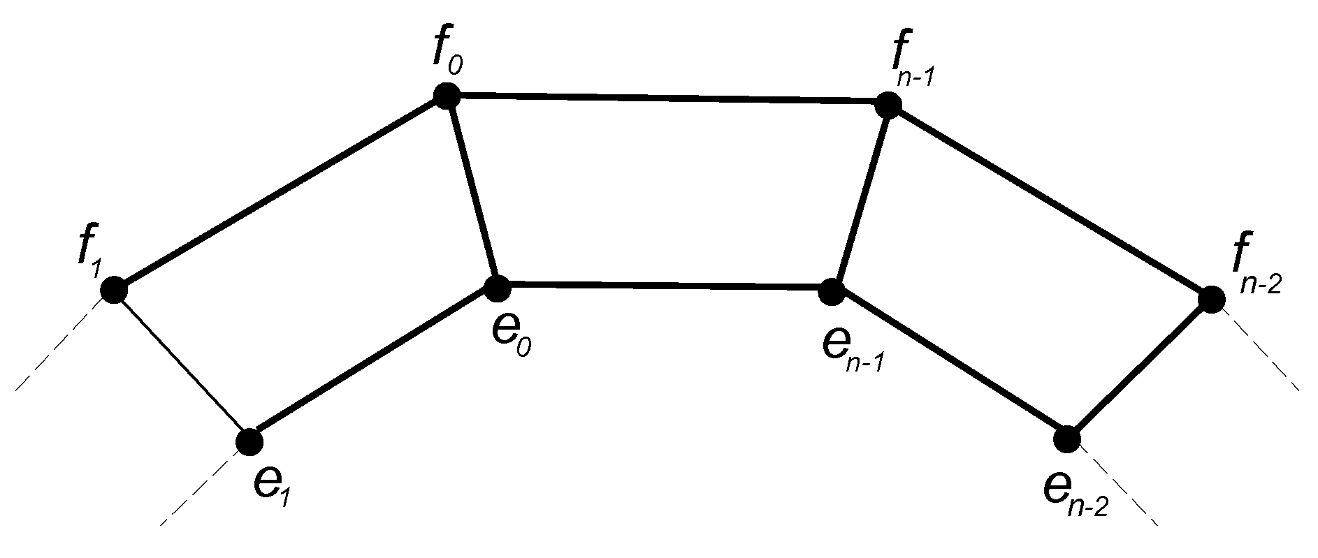
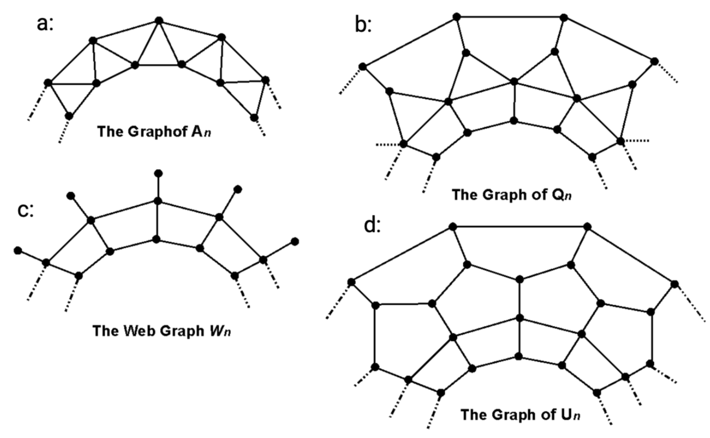
3.1. The Graph of Prism ${\mathcal{D}}_N$

The prism ${\mathcal{D}}_n$ is a 3-regular graph, as seen in Figure 1. It was studied in [13], and recently, this graph has been studied for the mixed metric dimension in [14]. The prism graph is generated by the Cartesian product of a cycle graph $C_n$ and a path graph $P_2$. The outer cycle comprises $f_0,f_1,\dots ,f_{n-1}$ vertices and an inner cycle $e_0,e_1,\dots ,e_{n-1}$.

The vertex set of $\mathcal{D}{}_n$ is

$$\begin{array}{c}\hfill V\left({\mathcal{D}}_n\right)=\{e_p,f_p\mid p=0,\dots ,n-1\}.\end{array}$$

The edge set of $\mathcal{D}{}_n$ is

$$\begin{array}{c}\hfill E\left({\mathcal{D}}_n\right)=\{(e_p,e_{p+1}),(e_p,e_{p-1}),,(e_p,f_p),(f_p,f_{p+1}),(f_p,f_{p-1})\mid p=0,\dots ,n-1\}.\end{array}$$

Theorem 2.

For $n\ge 6$, the ${\gamma }^{old}\left({\mathcal{D}}_n\right)$ is

$${\gamma }^{old}\left({\mathcal{D}}_n\right)=n$$

Proof. 

The prism graph ${\mathcal{D}}_n$ is a 3-regular graph. So, by Theorem 1, we have

$${\gamma }^{old}\left({\mathcal{D}}_n\right)\ge ⌈\frac{2\left(2n\right)}{4}⌉=n.$$

Let $S=\left\{f_p\right|p=0,1,\dots ,n-1\}$. It can be seen that all the intersections $S\cap N\left(e_p\right)=\left\{f_p\right\}$; $S\cap N\left(f_p\right)=\{f_{p-1},f_{p+1}\}$ are non-empty and distinct. Since the set S is an open locating-dominating set of the prism graph ${\mathcal{D}}_n$, we have $S=\left|n\right|$. Therefore, it can be deduced that ${\gamma }^{old}\left({\mathcal{D}}_n\right)\le n$. Keeping in mind the fact that we have ${\gamma }^{old}\left({\mathcal{D}}_n\right)\ge n$, it is proven that ${\gamma }^{old}\left({\mathcal{D}}_n\right)=n$. □

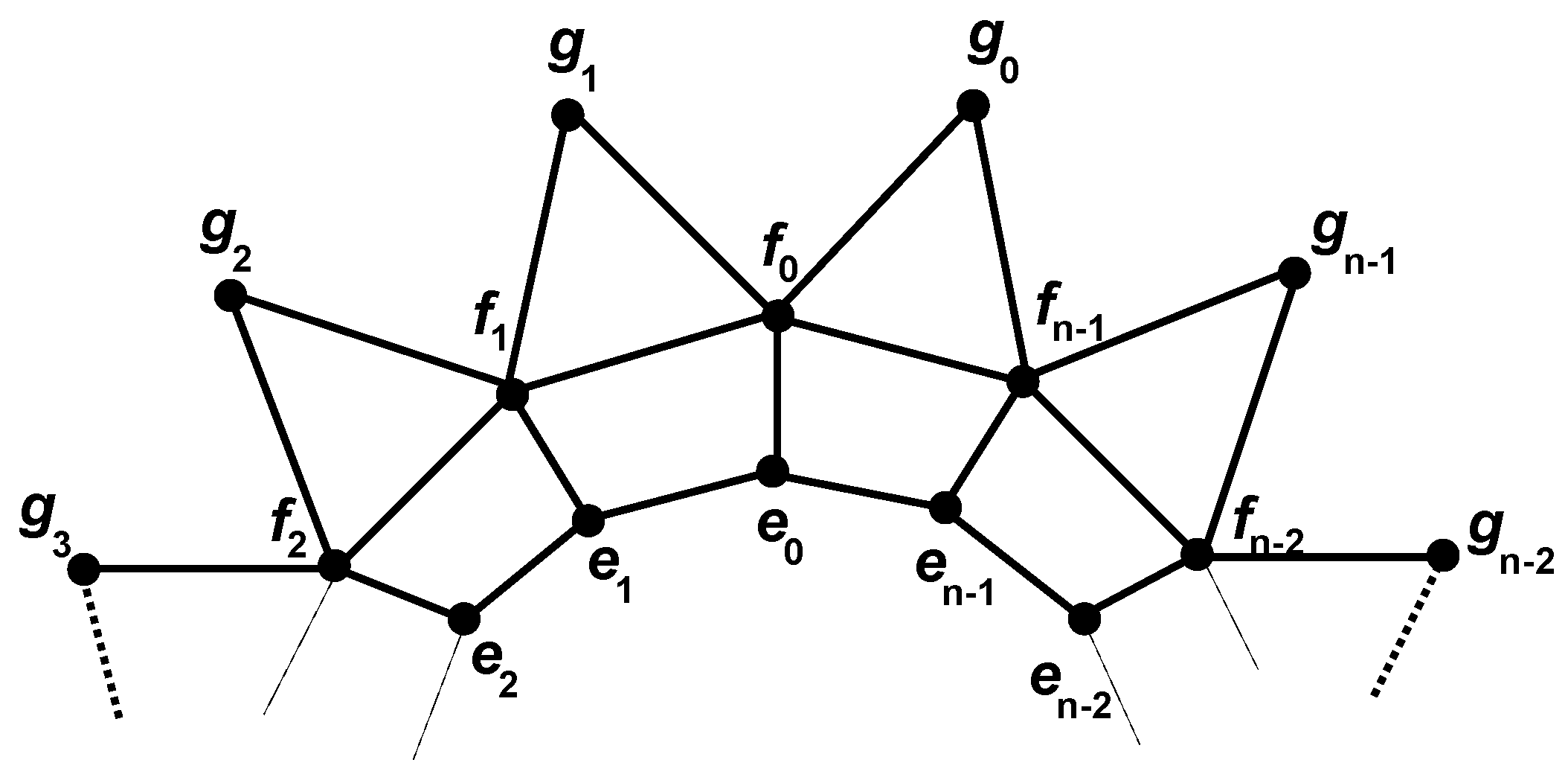
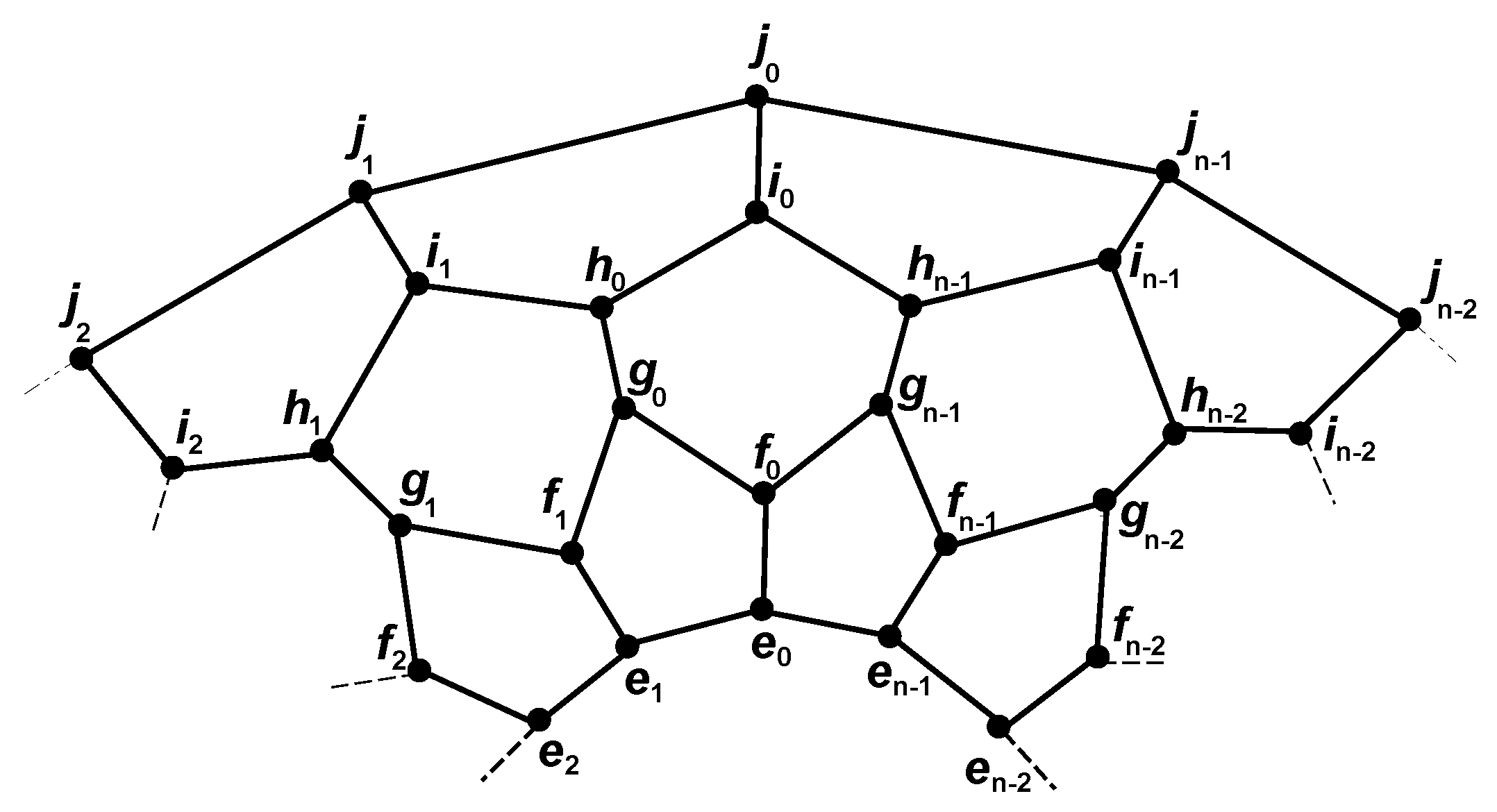
3.2. The Prism Related Graph ${\mathcal{D}}_N^{*}$

The plane graph ${\mathcal{D}}_n^{*}$, as seen in Figure 2, has been recently studied in [15]. It is an extension of the prism graph ${\mathcal{D}}_n$. The ${\mathcal{D}}_n^{*}$ is constructed. It is obtained by inserting a new vertex $g_p$ in the central vertices $f_{p-1}$ and $f_p$ of the external cycle with the vertex $g_p$ by joining the two vertices $f_{p-1}$ and $f_p$ for $0\le p\le n-1$. For the sake of simplicity, $f_0=f_{n-1}$. The set of vertices $e_p$, $f_p$ and $g_p$, are called internal, central and external vertices. The vertex set of ${\mathcal{D}}_n^{*}$ is

$$\begin{array}{c}\hfill V\left({\mathcal{D}}_n^{*}\right)=\{e_p,f_p,g_p\mid p=0,\dots ,n-1\}\end{array}$$

and the edge set of ${\mathcal{D}}_n^{*}$ is

$$\begin{array}{c}\hfill E\left({\mathcal{D}}_n^{*}\right)=\{(e_p,e_{p+1}),(e_p,e_{p-1}),(e_p,f_p),(f_p,f_{p+1}),(f_p,f_{p-1}),(f_p,g_p),(f_p,g_{p+1}),\mid p=0,\dots ,n-1\}.\end{array}$$

Theorem 3.

For $n\ge 4$, the ${\gamma }^{old}\left({\mathcal{D}}_n^{*}\right)$ is given as

$${\gamma }^{old}\left({\mathcal{D}}_n^{*}\right)=n$$

Proof. 

The plane graph ${\mathcal{D}}_n^{*}$ is the graph with the maximum degree five. Then, by Theorem 1, we have

$${\gamma }^{old}\left({\mathcal{D}}_n^{*}\right)\ge ⌈\frac{2\left(3n\right)}{6}⌉=n.$$

Let $S=\left\{f_p\right|p=0,1,\dots ,n-1\}$. It can be clearly seen that $S\cap N\left(e_p\right)=\left\{f_p\right\}$, $S\cap N\left(f_p\right)=\{f_{p-1},f_{p+1}\}$, $S\cap N\left(g_p\right)=\{f_{p-1},f_p\}$ are non-empty and distinct. Since the set S is an open locating-dominating set of the prism-related graph ${\mathcal{D}}_n^{*}$, we have $S=\left|n\right|$. Therefore, it can be deduced that ${\gamma }^{old}\left({\mathcal{D}}_n^{*}\right)\le n$. Keeping in mind the fact that we have ${\gamma }^{old}\left({\mathcal{D}}_n^{*}\right)\ge n$, it is proven that ${\gamma }^{old}\left({\mathcal{D}}_n^{*}\right)=n$. □

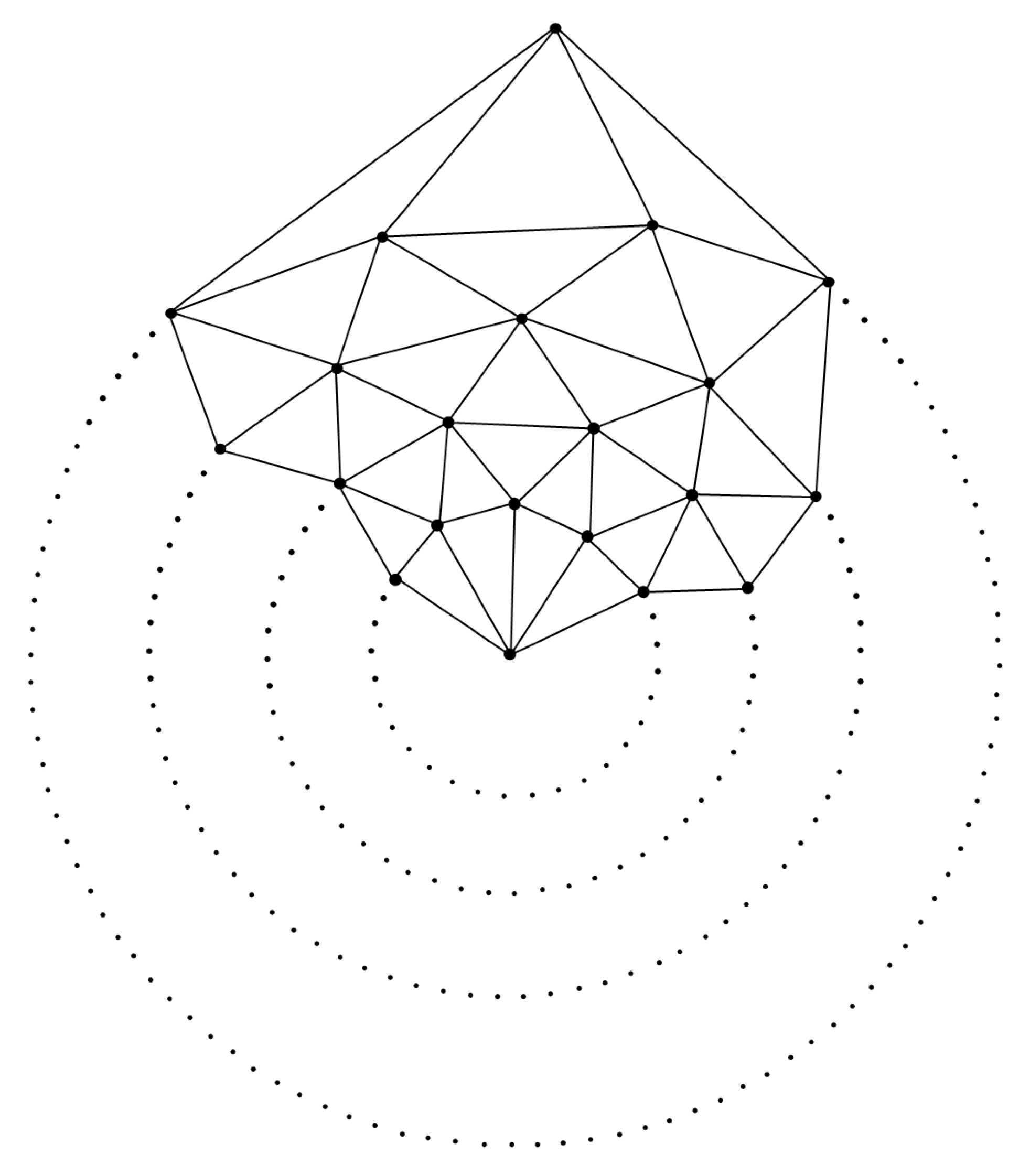
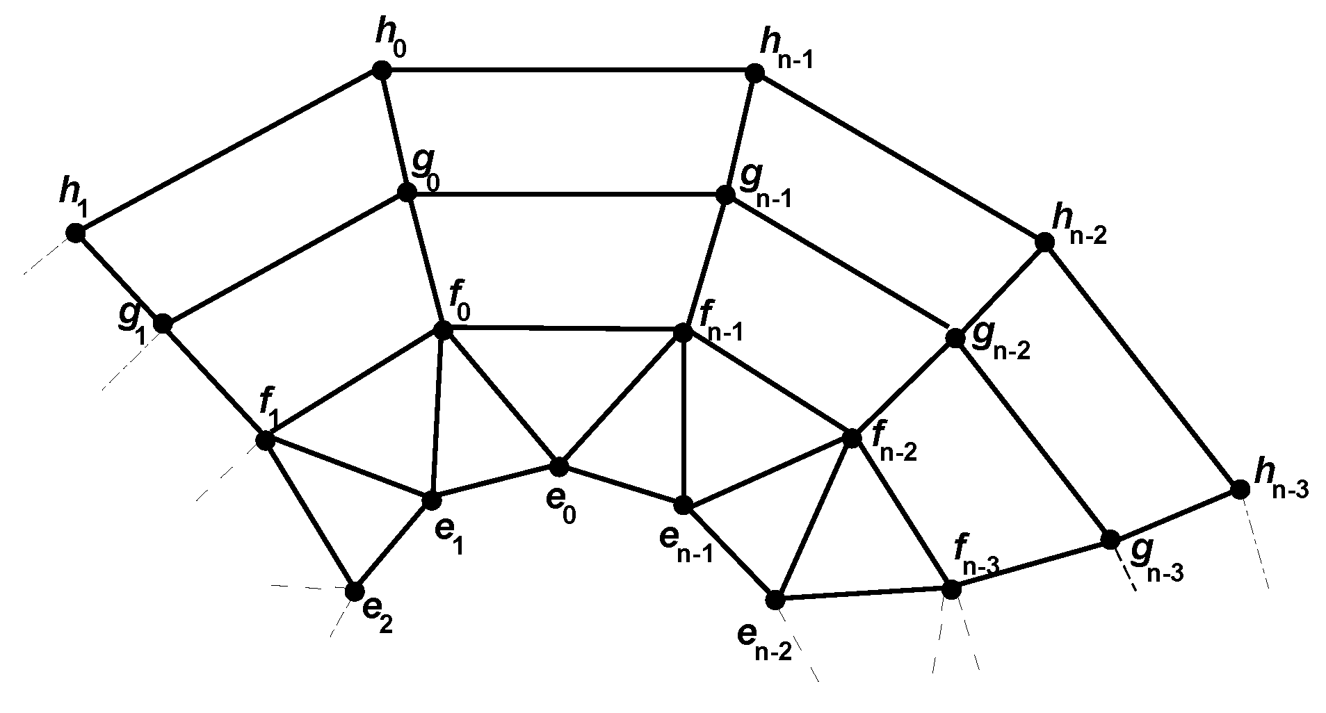
4. Exact Values of Convex Polytopes

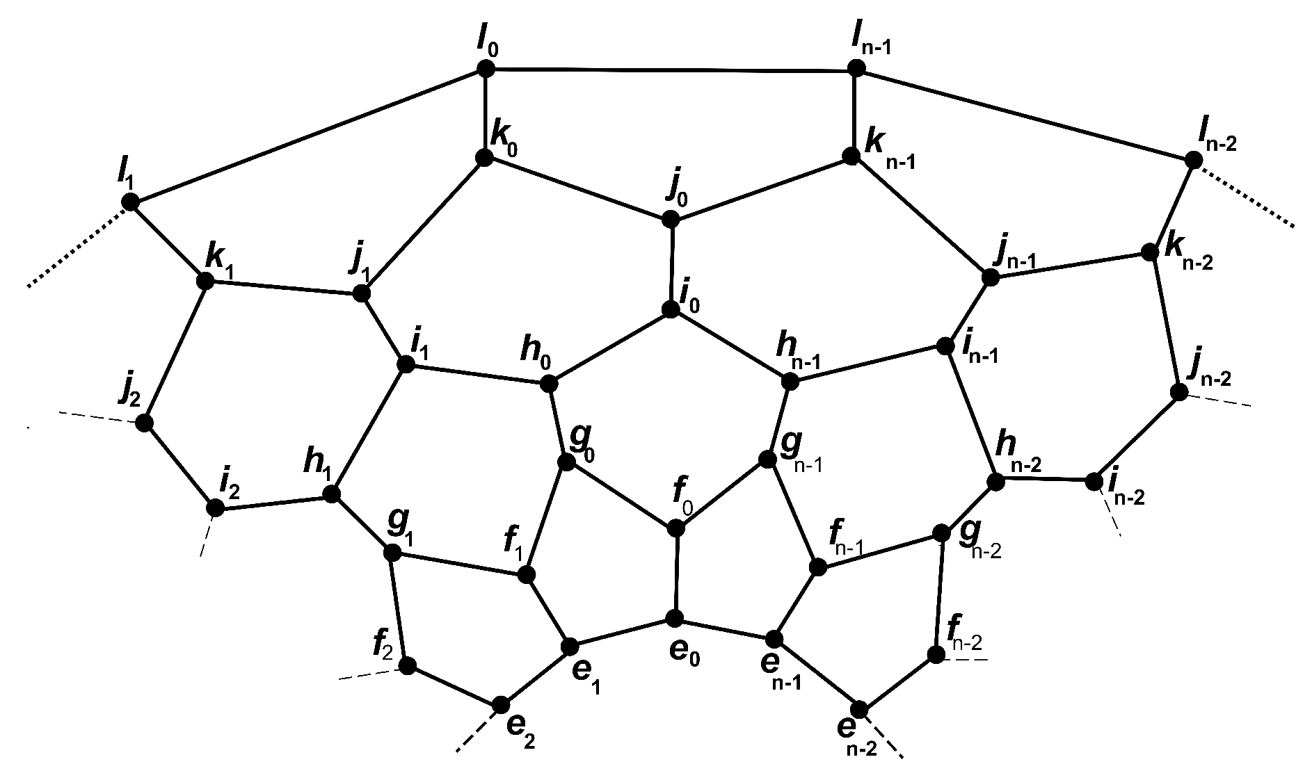
4.1. The Graph of Convex Polytopes ${\mathcal{R}}_n$

The labeling problem of ${\mathbb{B}}_n$ ($n\ge 3$), the graph associated with a family of convex polytopes, was studied by Bača [16] ($n\ge 3$). It is shown in Figure 3.

Miller et al. [17] studied different variations of $\mathbb{B}n$ by describing its dual, and the dual G represented as $du\left(G\right)$, for a given planar graph. The construction of G is performed by adding a vertex in the internal face of G. If their corresponding faces share an edge, then it should be joined. This new polytope is represented as ${\mathcal{R}}_n$. The family of graphs ${\mathcal{R}}_n$ can be generated from the graph of $D_n$ when a layer of hexagons is added between the two pentagonal layers. The graph of $D_n$ can be viewed in Figure 4.

The graph of a convex polytope ${\mathcal{R}}_n$, as shown in Figure 5, consists of $2n$ 5-sided faces, n 6-sided faces, and n-sided faces, as studied in Miller et al. [17]. The vertex set of ${\mathcal{R}}_n$ is

$$V\left({\mathcal{R}}_n\right)=\{e_p,f_p,g_p,h_p,i_p,j_p\mid p=0,\dots ,n-1\}.$$

The edge set of ${\mathcal{R}}_n$ is

$$\begin{array}{c}\hfill E\left({\mathcal{R}}_n\right)=\{e_p{e}_{p-1},e_p{e}_{p+1},e_p{f}_p,f_p{g}_{p-1},f_p{g}_p,g_p{h}_p,h_p{i}_p,\\ \hfill h_p{i}_{p+1},i_p{g}_p,j_p{j}_{p-1},j_p{j}_{p+1}\mid p=0,\dots ,n-1\}.\end{array}$$

Theorem 4.

For $n\ge 6$, we have

$${\gamma }^{old}\left({\mathcal{R}}_n\right)=3n$$

Proof. 

The graph of the convex polytope ${\mathcal{R}}_n$ is a 3-regular graph of degree 3. Then, by Theorem 1, we have ${\gamma }^{old}\left({\mathcal{R}}_n\right)\ge ⌈\frac{2\left(6n\right)}{4}⌉=3n$.

Let $S=\{e_p,h_p,i_p|p=0,1,\dots ,n-1\}$.

The

Table 3. Open locating-dominating vertices in ${\mathcal{R}}_n$.

v	$\mathit{S}\cap \mathit{N}\left(\mathit{v}\right)$
$e_p$	$\{e_{p-1},e_{p+1}\}$
$f_p$	$\left\{e_p\right\}$
$g_p$	$\left\{h_p\right\}$
$h_p$	$\{i_p,i_{p+1}\}$
$i_p$	$\{h_{p-1},h_p\}$
$j_p$	$\left\{i_p\right\}$

clearly shows that the intersections are non-empty and distinct.

So, the set S is an OLD-set of ${\mathcal{R}}_n$. So, $\left|S\right|=3n$, and therefore, ${\gamma }^{old}\left({\mathcal{R}}_n\right)\le 3n$. On the other hand, ${\gamma }^{old}\left({\mathcal{R}}_n\right)\ge 3n$. So, from all the above facts, it follows that ${\gamma }^{old}\left({\mathcal{R}}_n\right)=3n$.

The extension of the graph $D_n$ yields more families of regular graphs of convex polytopes by preserving the symmetric relation as shown in the Figure 6. □

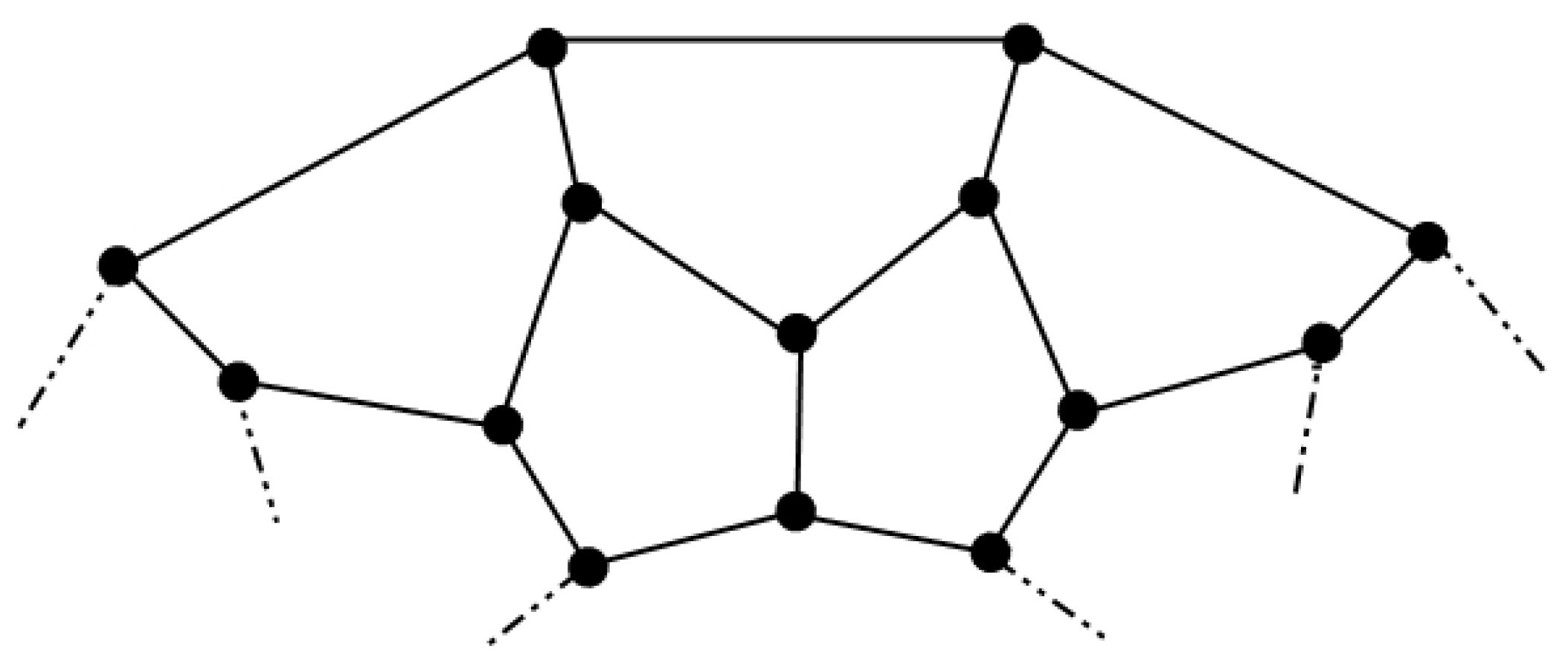
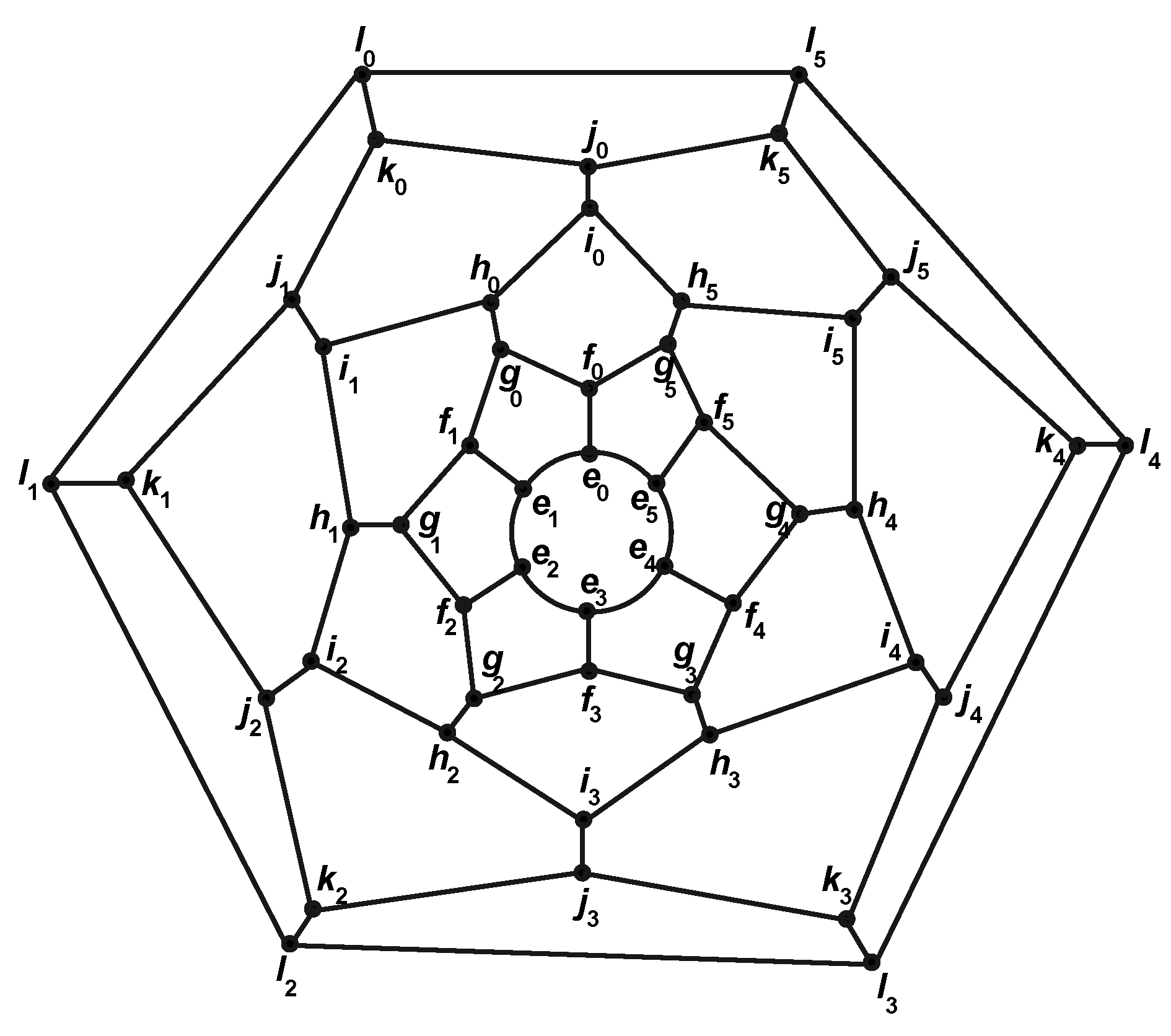
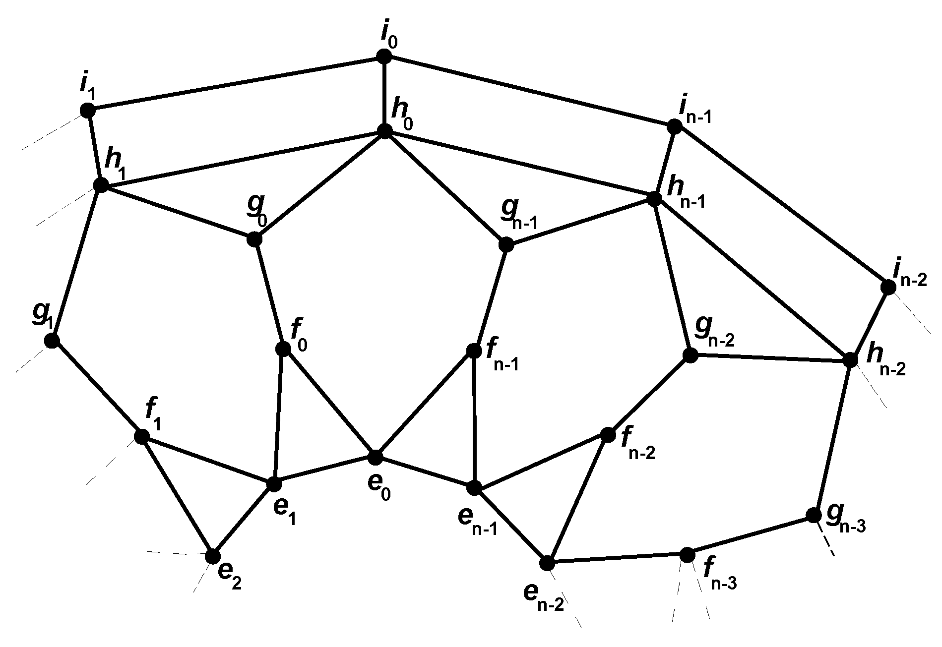
4.2. The Graph of Convex Polytope ${\mathcal{H}}_n$

Now, we study further variations of $D_n$ and the open locating-domination number for this family of graphs. In a similar fashion to Miller et al. [17], ${\mathcal{H}}_n$ is obtained by adding an extra layer of hexagons in between the lower hexagonal layer and the outer pentagonal layer, as seen in Figure 7. The graph of ${\mathcal{H}}_n$ consists of $2n$ pentagonal and hexagonal faces and also a pair of n-gonal faces.

The vertex set is

$$V\left({\mathcal{H}}_n\right)=\{e_p,f_p,g_p,h_p,i_p,j_p,k_p,l_p\mid p=0,\dots ,n-1\}.$$

The edge set is

$$\begin{array}{ccc}\hfill E\left({\mathcal{H}}_n\right)& =& \{e_p{e}_{p-1},e_p{e}_{p+1},e_p{f}_p,f_p{g}_p,f_p{g}_{p-1},\hfill \\ & & g_p{h}_p,h_p{i}_p,h_p{i}_{p+1},i_p{j}_p,j_p{k}_{p-1},\hfill \\ & & j_p{k}_p,k_p{l}_p,l_p{l}_{p-1},l_p{i}_{p+1}\mid p=0,1,\dots ,n-1.\}\hfill \end{array}$$

Now, we will validate the vertex and the edge set of the graph ${\mathcal{H}}_n$ by fixing $n=6$, and draw the graph ${\mathcal{H}}_6$.

The vertex set of ${\mathcal{H}}_6$ is

$$V\left({\mathcal{H}}_6\right)=\{e_0,\dots ,e_5,f_0,\dots ,f_5,g_0,\dots ,g_5,h_0,\dots ,h_5,i_0,\dots ,i_5,j_0,\dots ,j_5,k_0,\dots ,k_5,l_0,\dots ,l_5\}.$$

The edge set of ${\mathcal{H}}_6$ is

$$\begin{array}{ccc}\hfill E\left({\mathcal{H}}_6\right)& =& \{e_0{e}_1,e_1{e}_2,e_2{e}_3,e_3{e}_4,e_4{e}_5,e_5{e}_0,e_0{f}_0,e_1{f}_1,e_2{f}_2,e_3{f}_3,e_4{f}_4,e_5{f}_5,f_0{g}_0,f_1{g}_1,f_2{g}_2,f_3{g}_3,f_4{g}_4,f_5{g}_5,\hfill \\ & & f_0{g}_5,f_1{g}_0,f_2{g}_1,f_3{g}_2,f_4{g}_3,f_5{g}_4,g_0{h}_0,g_1{h}_1,g_2{h}_2,g_3{h}_3,g_4{h}_4,g_5{h}_5,i_0{h}_0,i_1{h}_1,i_2{h}_2,i_3{h}_3,\hfill \\ & & i_4{h}_4,i_5{h}_5,i_0{h}_5,i_1{h}_0,i_2{h}_1,i_3{h}_2,i_4{h}_3,i_5{h}_4,i_0{j}_0,i_1{j}_1,i_2{j}_2,i_3{j}_3,i_4{j}_4,i_5{j}_5,j_0{k}_0,\hfill \\ & & j_1{k}_1,j_2{k}_2,j_3{k}_3,j_4{k}_4,j_5{k}_5,j_0{k}_5,j_1{k}_0,j_2{k}_1,j_3{k}_2,j_4{k}_3,j_5{k}_4,k_0{l}_0,k_1{l}_1,k_2{l}_2,k_3{l}_3,\hfill \\ & & k_4{l}_4,k_5{l}_5,l_0{l}_1,l_1{l}_2,l_2{l}_3,l_3{l}_4,l_4{l}_5,l_5{l}_0\}.\hfill \end{array}$$

The graph of the convex polytope ${\mathcal{H}}_6$ is constructed by using the vertex and edge sets as shown in Figure 8.

Theorem 5.

For $n\ge 8$, we have

$${\gamma }^{old}\left({\mathcal{H}}_n\right)=4n$$

Proof. 

The graph of the convex polytope ${\mathcal{H}}_n$ is a 3-regular graph of degree 3. Then, by Theorem 1, we have ${\gamma }^{old}\left({\mathcal{H}}_n\right)\ge ⌈\frac{2\left(8n\right)}{4}⌉=4n$.

Let $S=\{e_p,h_p,i_p,l_p|p=0,1,\dots ,n-1\}$.

The

Table 4. Open locating-dominating vertices in ${\mathcal{H}}_n$.

v	$\mathit{S}\cap \mathit{N}\left(\mathit{v}\right)$
$e_p$	$\{e_{p-1},e_{p+1}\}$
$f_p$	$\left\{e_p\right\}$
$g_p$	$\left\{h_p\right\}$
$h_p$	$\{i_p,i_{p+1}\}$
$i_p$	$\{h_{p-1},h_p\}$
$j_p$	$\left\{i_p\right\}$
$k_p$	$\left\{l_p\right\}$
$l_p$	$\{l_{p+1},l_{p-1}\}$

clearly shows that the intersections are non-empty and distinct.

So, the set S is an open locating-dominating set of ${\mathcal{H}}_n$. So, $\left|S\right|=4n$, and therefore, ${\gamma }^{old}\left({\mathcal{H}}_n\right)\le 4n$. On the other hand, ${\gamma }^{old}\left({\mathcal{H}}_n\right)\ge 4n$. From all these above facts, it follows that ${\gamma }^{old}\left({\mathcal{H}}_n\right)=4n$. □

Remark. 

Further extension of the graph $D_n$, as seen inFigure 6, yields more classes of regular convex polytopes, and we claim that all these families of convex polytopes have exact values for the open locating-dominating number.

5. Upper Bounds

5.1. The Graph of Convex Polytope ${\mathcal{S}}_n$

The graph of the convex polytope $S_n$ is composed of $2n$ trigonal, $2n$ 4-gonal and a pair of n-sided faces. A recent study for this class of convex polytopes has been carried out in [18], see Figure 9. Now, the vertex set of ${\mathcal{S}}_n$ is

$$V\left({\mathcal{S}}_n\right)=\{e_p,f_p,g_p,h_p\mid p=0,\dots ,n-1\}.$$

The edge set of ${\mathcal{S}}_n$ is

$$\begin{array}{c}\hfill E\left({\mathcal{S}}_n\right)=\{e_p{e}_{p+1},e_p{e}_{p-1},e_p{f}_p,e_p,f_{p-1},f_p,f_{p+1}\mid p=0,\dots ,n-1\}\cup \\ \hfill \{f_p{f}_{p-1},f_p{g}_p,g_p{g}_{p+1},g_p{g}_{p-1},g_p{h}_p,h_p{h}_{p+1},h_p{h}_{p-1}\mid p=0,\dots ,n-1\}.\end{array}$$

An upper bound is presented for ${\mathcal{S}}_n$.

Theorem 6.

For $n\ge 6$, for the graph of the convex polytope $S_n$, we have

$${\gamma }^{old}\left({\mathcal{S}}_n\right)\le \left\{\begin{array}{cc}⌈\frac{5n}{3}⌉,\hfill & n\equiv 0,2(mod3);\hfill \\ ⌈\frac{5n}{3}⌉+1,\hfill & n\equiv 1(mod3).\hfill \end{array}\right.$$

Proof. 

We consider three cases.

Case 1: When $n=3q$, and $q\ge 2$. Let $S=\{f_p\mid p=0,\dots ,n-1\}\cup \{h_{3p+1},h_{3p+2}\mid p=0,$$\dots ,q-1\}$.

Case 2: When $n=3q+1$, and $q\ge 2$. Let $S=\{f_p\mid p=0,\dots ,n-1\}\cup \{h_{3p},h_{3p+1}\mid p=0,$$\dots ,q-1\}\cup \{h_{3q-1},h_{3q}\}$.

Case 3: When $n=3q+2$, and $q\ge 2$. Let $S=\{f_p\mid p=0,\dots ,n-1\}\cup \{h_{3p},h_{3p+1}\mid p=0,$$\dots ,q-1\}\cup \{h_{3q},h_{3q+1}\}$.

The

Table 5. Open locating-dominating vertices in ${\mathcal{S}}_n$.

n	v	$\mathit{S}\cap \mathit{N}\left(\mathit{v}\right)$
$3q$	$e_p$	$\{f_{p-1},f_p\}(p=0,\dots ,n-1$)
	$f_p$	$\{f_{p-1},f_{p+1}\}(p=0,\dots ,n-1$)
	$g_{3p}$	$\left\{f_{3p}\right\}$
	$g_{3p+1}$	$\{f_{3p+1},h_{3p+1}\}$
	$g_{3p+2}$	$\{f_{3p+2},h_{3p+2}\}$
	$h_{3p+1}$	$\left\{h_{3p+2}\right\}$
	$h_{3p+2}$	$\left\{h_{3p+1}\right\}$
	$h_{3p+3}(p=0,\dots ,q-2)$	$\{h_{3p+2},h_{3p+4}\}(p=0,\dots ,q-2)$
	$h_0$	$\{h_1,h_{3q-1}\}$
$3q+1$	$e_p$	$\{f_{p-1},f_p\}(p=0,\dots ,n-1$)
	$f_p$	$\{f_{p-1},f_{p+1}\}(p=0,\dots ,n-1$)
	$g_{3p}(p=0,\dots ,q)$	$\{f_{3p},h_{3p}\}(p=0,\dots ,q)$
	$g_{3p+1}$	$\{f_{3p+1},h_{3p+1}\}$
	$g_{3p+2}(p=0,\dots ,q-2)$	$\left\{f_{3p+2}\right\}(p=0,\dots ,q-2)$
	$h_{3p+1}(p=0,\dots ,q-2)$	$\left\{h_{3p}\right\}(p=0,\dots ,q-2)$
	$h_{3p+2}$	$\{h_{3p+1},h_{3p+3}\}$
	$h_{3p+3}$	$\left\{h_{3p+4}\right\}$
	$g_{3q-1}$	$\{f_{3q-1},h_{3q-1}\}$
	$h_{3q-2}$	$\{h_{3q-3},h_{3q-1}\}$
	$h_{3q}$	$\{h_{3q-1},h_0\}$
	$h_0$	$\{h_1,h_{3q}\}$
$3q+2$	$e_p$	$\{f_{p-1},f_p\}(p=0,\dots ,n-1$)
	$f_p$	$\{f_{p-1},f_{p+1}\}(p=0,\dots ,n-1$)
	$g_{3p}(p=0,\dots ,q)$	$\{f_{3p},h_{3p}\}(p=0,\dots ,q)$
	$g_{3p+1}(p=0,\dots ,q)$	$\{f_{3p+1},h_{3p+1}\}(p=0,\dots ,q)$
	$g_{3p+2}$	$\left\{f_{3p+2}\right\}$
	$h_{3p+1}$	$\left\{h_{3p}\right\}$
	$h_{3p+2}$	$\{h_{3p+1},h_{3p+3}\}$
	$h_{3p+3}$	$\left\{h_{3p+4}\right\}$
	$h_0$	$\{h_{3q+1},h_1\}$
	$h_{3q+1}$	$\{h_{3q},h_0\}$

clearly shows that in all these cases the intersections are non-empty and distinct. □

5.2. The Graph of Convex Polytope ${\mathcal{R}}_n^{\prime }$

The graph of the convex polytope ${\mathcal{R}}_n^{\prime }$ consists of $2n$ 3-sided faces, n 4-sided faces, n 6-sided faces, trigonal faces, and a pair of n-sided faces, as studied [19].The notation for this class of convex polytopes is $R_n$ and, to avoid ambiguity, we use ${\mathcal{R}}_n^{\prime }$, see Figure 10. Mathematically, the vertex set of ${\mathcal{R}}_n^{\prime }$ is

$$V\left({\mathcal{R}}_n^{\prime }\right)=\{e_p,f_p,g_p,h_p,i_p\mid p=0,\dots ,n-1\}.$$

The edge set ${\mathcal{R}}_n^{\prime }$ is

$$\begin{array}{c}\hfill E\left({\mathcal{R}}_n^{\prime }\right)=\{e_p{e}_{p+1},e_p{e}_{p-1},e_p{f}_p,e_p,f_{p-1},f_p,g_p\}\cup \\ \hfill \{g_p{h}_p,g_p{h}_{p+1},h_p{h}_{p-1},h_p{h}_{p+1},h_p{i}_p,i_p{i}_{p+1},i_p{i}_{p-1}\mid p=0,\dots ,n-1\}.\end{array}$$

Theorem 7.

For $n\ge 6$, the graph of the convex polytope ${\mathcal{R}}_n^{\prime }$,

$${\gamma }^{old}\left({\mathcal{R}}_n^{\prime }\right)\le 2n.$$

Proof. 

Let $S=\{e_p,h_p|p=0,1,\dots ,n-1\}$.

It can be clearly seen from

Table 6. Open locating-dominating vertices in ${\mathcal{R}}_n^{\prime }$.

v	$\mathit{S}\cap \mathit{N}\left(\mathit{v}\right)$
$e_p$	$\{e_{p-1},e_{p+1}\}$
$f_p$	$\{e_p,e_{p+1}\}$
$g_p$	$\{h_p,h_{p+1}\}$
$h_p$	$\{h_{p-1},h_{p+1}\}$
$i_p$	$\left\{h_p\right\}$

that all the intersections of vertices with the set S are non-empty and distinct. So, $S=\left|2n\right|$, and thus, ${\mathcal{R}}_n^{\prime }\le 2n$. Therefore, we obtain that ${\gamma }^{old}\left({\mathcal{R}}_n^{\prime }\right)\le 2n$. □

Theorem 8.

(i) For $n\ge 6$, the graph of convex polytopes ${\mathcal{A}}_n$,

$${\gamma }^{old}\left({\mathcal{A}}_n\right)\le n-1.$$

(ii) For $n\ge 6$, the web graph ${\mathbb{W}}_n$,

$${\gamma }^{old}\left({\mathbb{W}}_n\right)\le \left\{\begin{array}{cc}⌈\frac{3n}{2}⌉,\hfill & n\equiv 0,1,3(mod4);\hfill \\ ⌈\frac{3n}{2}⌉+1\hfill & n\equiv 2(mod4).\hfill \end{array}\right.$$

(iii) For $n\ge 6$, the graph of convex polytopes ${\mathcal{Q}}_n$,

$${\gamma }^{old}\left({\mathcal{Q}}_n\right)\le \left\{\begin{array}{cc}⌈\frac{5n}{3}⌉,\hfill & n\equiv 0,2(mod3);\hfill \\ ⌈\frac{5n}{3}⌉+1\hfill & n\equiv 1(mod3).\hfill \end{array}\right.$$

(iv) For $n\ge 6$, the graph of convex polytopes ${\mathcal{U}}_n$,

$${\gamma }^{old}\left({\mathcal{U}}_n\right)\le \left\{\begin{array}{cc}⌈\frac{8n}{3}⌉,\hfill & n\equiv 0,2(mod3);\hfill \\ ⌈\frac{8n}{3}⌉+1\hfill & n\equiv 1(mod3).\hfill \end{array}\right.$$

Proof. 

The proofs for the graphs of ${\mathcal{A}}_n$, ${\mathbb{W}}_n$, ${\mathcal{Q}}_n$, and ${\mathcal{U}}_n$ are similar. For the structural properties of these graphs, see Figure 11. □

6. Conclusions

In this paper, we improved the result for the OLD-set and the value of ${\gamma }^{old}\left(C_n\right)$ cycle graphs when $n\equiv 1\left(\mathrm{mod}3\right)$. The exact values of ${\gamma }^{old}\left(G\right)$ for the graphs of prism ${\mathcal{D}}_n$, and prism-related graphs ${\mathcal{D}}_n^{*}$ are attained. Furthermore, the exact values are also attained for the graphs of the convex polytopes ${\mathcal{R}}_n$ and ${\mathcal{H}}_n$. The upper bounds are computed for the graphs of the convex polytopes ${\mathcal{S}}_n$, ${\mathcal{R}}_n^{\prime }$, ${\mathcal{A}}_n$, ${\mathcal{Q}}_n$, and ${\mathcal{U}}_n$ and also for the web graph ${\mathbb{W}}_n$.

Future research can focus on the different invariants of domination-related parameters for the classes of convex polytopes. The open locating-dominating set can be considered for more challenging classes of graphs.

References

1. Cappelle, M.R.; Coelho, E.M.; Foulds, L.R.; Longo, H.J. Open-independent, Open-locating-dominating Sets in Complementary Prism Graphs. Electron. Notes Theor. Comput. Sci. 2019, 346, 253–264. [Google Scholar] [CrossRef]
2. Seo, S.J.; Slater, P.J. Open-independent, open-locating-dominating sets. Electron. J. Graph Theor. Appl. 2017, 5, 179–193. [Google Scholar] [CrossRef] [Green Version]
3. Seo, S.J.; Slater, P.J. Open neighborhood locating-dominating in trees. Discret. Appl. Math. 2011, 159, 484–489. [Google Scholar] [CrossRef] [Green Version]
4. Seo, S.J.; Slater, P.J. Open Locating-Dominating Interpolation for Trees. Congressus Numerantium 2013, 215, 145–152. [Google Scholar]
5. Slater, P.J. Dominating and reference sets in a graph. J. Math. Phys. Sci. 1988, 22, 445–455. [Google Scholar]
6. Karpovsky, M.G.; Krishnendu, C.; Lev, B.L. On a new class of codes for identifying vertices in graphs. IEEE Trans. Inf. Theor. 1998, 44, 599–611. [Google Scholar] [CrossRef] [Green Version]
7. Seo, S.J.; Slater, P.J. Open neighborhood locating dominating sets. Australas. J. Combinat. 2010, 46, 109–120. [Google Scholar]
8. Chellali, M.; Rad, N.J.; Seo, S.J.; Slater, P.J. On open neighborhood locating-dominating in graphs. Electron. J. Graph Theor. Appl. (EJGTA) 2014, 2, 87–98. [Google Scholar] [CrossRef] [Green Version]
9. Raza, H.; Hayat, S.; Pan, X.F. Binary locating-dominating sets in rotationally-symmetric convex polytopes. Symmetry 2018, 10, 727. [Google Scholar] [CrossRef] [Green Version]
10. Simić, A.; Bogdanović, M.; Milošević, J. The binary locating-dominating number of some convex polytopes. Mathematica Contemporanea 2017, 13, 367–377. [Google Scholar] [CrossRef]
11. Savič, A.; Maksimovič, Z.; Bogdanovič, M. The open-locating-dominating number of some convex polytopes. Filomat 2018, 32, 635–642. [Google Scholar] [CrossRef]
12. Argiroffo, G.; Bianchi, S.; Lucarini, Y.; Wagler, A. The identifying code, the locating-dominating, the open locating-dominating and the locating total-dominating problems under some graph operations. Electron. Notes Theor. Comput. Sci. 2019, 346, 135–145. [Google Scholar] [CrossRef]
13. Gallian, J.A. Dynamic Survey DS6: Graph Labeling. Electron. J. Comb. 2007, DS 6, 1–58. [Google Scholar]
14. Raza, H.; Jia, B.; Liu, Q.S. On Mixed Metric Dimension of Rotationally Symmetric Graphs. IEEE Access 2019, 8, 11560–11569. [Google Scholar] [CrossRef]
15. Zhang, Y.; Gao, S. On the edge metric dimension of convex polytopes and its related graphs. J. Combinat. Optim. 2020, 39, 334–350. [Google Scholar] [CrossRef]
16. Bača, M. Face anti-magic labelings of convex polytopes. Utilitas Math. 1999, 55, 221–226. [Google Scholar]
17. Miller, M.; Bača, M.; MacDougall, J.A. Vertex-magic total labeling of generalized Petersen graphs and convex polytopes. J. Combin. Math. Combin. Comput. 2006, 59, 89–99. [Google Scholar]
18. Raza, H.; Hayat, S.; Pan, X.F. On the fault-tolerant metric dimension of convex polytopes. Appl. Math. Comput. 2018, 339, 172–185. [Google Scholar] [CrossRef]
19. Malik, M.; Aslam, M.S. On the metric dimension of two families of convex polytopes. Afrika Matematika 2016, 27, 229–238. [Google Scholar] [CrossRef] [Green Version]
Figure 1. The graph of D n .
Mathematics 09 01415 g001
Figure 2. The graph of D n * .
Mathematics 09 01415 g002
Figure 3. The graph of convex polytope B n .
Mathematics 09 01415 g003
Figure 4. The graph of convex polytope D n .
Mathematics 09 01415 g004
Figure 5. The graph of convex polytope R n .
Mathematics 09 01415 g005
Figure 6. Extension of the graph D n .
Mathematics 09 01415 g006
Figure 7. The graph of convex polytope H n .
Mathematics 09 01415 g007
Figure 8. The graph of convex polytope H 6 .
Mathematics 09 01415 g008
Figure 9. The graph of convex polytope S n .
Mathematics 09 01415 g009
Figure 10. The graph of convex polytope R n .
Mathematics 09 01415 g010
Figure 11. (a) The graph of convex polytope A n . (b) The graph of convex polytope Q n . (c) The web graph W n . (d) The graph of convex polytope U n .
Mathematics 09 01415 g011