On the Maximal Shortest Paths Cover Number

Abstract

A shortest path P of a graph G is maximal if P is not contained as a subpath in any other shortest path. A set $S\subseteq V\left(G\right)$ is a maximal shortest paths cover if every maximal shortest path of G contains a vertex of S. The minimum cardinality of a maximal shortest paths cover is called the maximal shortest paths cover number and is denoted by $\xi \left(G\right)$. We show that it is NP-hard to determine $\xi \left(G\right)$. We establish a connection between $\xi \left(G\right)$ and several other graph parameters. We present a linear time algorithm that computes exact value for $\xi \left(T\right)$ of a tree T.

1. Introduction and Preliminaries

Distance is one of essential terms in mathematics and has inspired many important results in different areas of mathematics. As the concept comes from real life, this gives rise to several applications. A theoretical model for a possible scenario of such an application is presented also in this work. Consider a complex system that can be modeled by a graph. When it is not possible to control every part of a system, usually due to technical or economical reasons, one would like to position the control points to strategic places of the underlying graph. We propose here to put these controls into the particular elements of the system, represented by vertices of a graph, in such a way that all the maximal shortest paths of the graph can be monitored and controlled from these elements.

In this work we consider finite simple graphs. Let G be a graph and $u,v$ be vertices of G. The distance between two vertices $u,v\in V\left(G\right)$ is the minimum number of edges on a path that starts at u and ends at v and is denoted by $d_G(u,v)$ or for short $d(u,v)$. A vertex $x\in V\left(G\right)$ strongly distinguishes vertices u and v of G if u is on a shortest path between x and v or v is on a shortest path between x and u. Set S is a strong metric generator if for any pair $u,v$ of different vertices of G there exists $x\in S$ such that x strongly distinguishes u and v. The minimum cardinality of a strong metric generator is called the strong metric dimension of G and is denoted by $\mathrm{sdim}\left(G\right)$. The strong metric dimension was introduced in [1], but later, in [2], Oellermann and Peters-Fransen connected strong metric dimension with so-called mutually maximal distant pairs of vertices. Vertices u and v form such a pair if the distance between v and every neighbor w of u does not exceed $d(u,v)$ and symmetrically if the distance between u and every neighbor w of v does not exceed $d(u,v)$. But this simply means that a shortest path P between u and v is a maximal shortest path, meaning that P is not included in any other longer shortest path as a subpath.

In [2] the authors also showed that $\mathrm{sdim}\left(G\right)$ is the minimum number of vertices that cover every mutually maximal distant pair of vertices. This approach was later more developed in several other papers (see, e.g., [3,4,5,6,7] for a flavor). Here we relax the conditions mentioned above and we only require that all maximal shortest paths in a graph are covered. One can wonder whether this requirement really leads to a relaxation. Indeed, there could be many shortest paths between the same pair of vertices. However, we can always take one vertex of a considered pair of vertices and it obviously lies on all maximal shortest paths between them in G. Hence, in this way we can cover all maximal shortest paths with a set of cardinality $\mathrm{sdim}\left(G\right)$. Therefore, our approach actually yields to a relaxation of maximal distant pair cover.

Such an approach is also a generalization of another well-known concept, namely the vertex cover number of a graph G that belongs to the essential 21 NP-complete problems described by Karp in [8]. We recall that the vertex cover number $\beta \left(G\right)$ is the minimum number of vertices that cover all edges of a graph G. Here we need to limit ourselves to graphs without isolated vertices, because every isolated vertex forms a maximal shortest path of length zero, but it does not contribute to $\beta \left(G\right)$. On the other hand, every other maximal shortest path contains at least one edge $e\in E\left(G\right)$ and at least one end-vertex of e must be contained in a vertex cover of G. The other generalization of the minimum vertex cover was introduced in [9]. The k-path vertex cover number ${\psi }_k\left(G\right)$ denotes the minimum cardinality of a minimal set of vertices of G that have a non-empty intersection with a vertex set of every path of order k. One can easily see that ${\psi }_1\left(G\right)$ and ${\psi }_2\left(G\right)$ coincide with the order of G and $\beta \left(G\right)$, respectively. For results concerning k-path vertex cover for product of graphs see, e.g., [10,11,12] and relationships to other invariants can be found in [13].

The same topic as it is considered in this paper was recently studied in [14] under the name The geodesic-transversal problem. Some results from the mentioned paper overlap with the results from this work; however, the used methods are different. The other results on maximal shortest paths cover can be found in [15], where the maximal shortest paths cover number is investigated for the joins and lexicographic products of two graphs.

A wheel graph $W_n$, $n\ge 4$, is a graph obtained from a cycle $C_{n-1}=v_1\dots v_{n-1}{v}_1$ by adding a new vertex u and edges $v_{i}u$ for every $i\in \{1,\dots ,n-1\}$. The vertex u of $W_n$ is universal and is called the central vertex of $W_n$. A star $S_k$, $k\ge 2$, is a special kind of complete bipartite graph, namely $K_{1,k-1}$. For some positive integers $k,t_1,\dots ,t_k$ a generalized star is a graph $S_{t_1,\dots ,t_k}$ with the central vertex v of degree k and with $S_{t_1,\dots ,t_k}-v$ isomorphic to k paths $P_{k_1},\dots ,P_{k_t}$. It is easy to see that if $t_1=\cdots =t_k=1$, then $S_{t_1,\dots ,t_k}\cong S_k$.

A grid graph or a Cartesian product of two paths $P_q\square P_r$ has vertices $v_{i,j}$ where $i\in \{1,\dots ,q\}$ and $j\in \{1,\dots ,r\}$. Two vertices $v_{i,j}$ and $v_{k,\ell }$ of $P_q\square P_r$ are adjacent if either $|i-k|=1$ and $j=\ell$ or $i=k$ and $|j-\ell |=1$. In [7] (see Proposition 30) among other results, also the strong metric dimension of grids was determined as

$$\mathrm{sdim}(P_q\square P_r)=2.$$

(1)

2. Definition and Complexity

A path between u and v of length $d(u,v)$ is called a $u,v$-shortest path or a $u,v$-geodesic. The diameter of G is denoted by $\mathrm{diam}\left(G\right)$ and is the length of a longest geodesic in G. A $u,v$-geodesic P is said to be extendible if there exist vertices $x,y$ in G such that $\{u,v\}\ne \{x,y\}$ and P is a subpath of a $x,y$-geodesic. If a path P is not extendible, then P is not contained in any other shortest path and is therefore a maximal shortest path. If there exists a maximal shortest path between u and v, then all $u,v$-geodesics are maximal shortest paths. 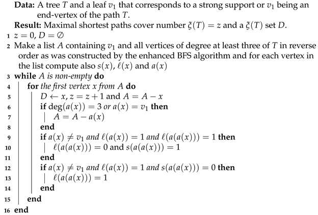The path $yxt$ at Figure 1 is extendible because it is a proper subpath of the path $yxtv$—a shortest path between y and v. The path $zxt$ is not extendible because it is not a proper subpath of any shortest path of the graph.

A subset S of the set of vertices of a graph G is called a maximal shortest paths cover if it has non-empty intersection with vertex set of every maximal shortest path of G. The vertex set $\{z,t\}$ at Figure 1 is the maximal shortest paths cover of the given graph since the paths $yxtv$ and $yzuv$ and $zxt$ are maximal shortest paths (i.e., the cardinality of the cover must be at least 2) and the paths $yx$ and $uv$ are extendible.

The cardinality of a smallest maximal shortest paths cover in a graph G is denoted by $\xi \left(G\right)$ and is called the maximal shortest paths cover number of G. Every maximal shortest paths cover of G of cardinality $\xi \left(G\right)$ is called a $\xi \left(G\right)$ set.

Let G and H be two graphs. The disjoint union of G and H is the graph $G\cup H$ that is obtained from one copy of G and one copy of H. The following observation ensures that it is enough to handle connected graphs. It holds because every maximal shortest path of $G\cup H$ is contained either in G or in H.

Proposition 1.

If G and H are arbitrary disjoint graphs, then $\xi (G\cup H)=\xi \left(G\right)+\xi \left(H\right)$.

We start with determining $\xi \left(G\right)$ for some classic families of graphs to get a better grip on the problem.

Proposition 2.

If k is a positive integer, then

(i) 

$\xi \left(P_k\right)=1$, $k\ge 1$;

(ii) 

$\xi \left(C_k\right)=2$, $k\ge 3$;

(iii) 

$\xi \left(S_k\right)=1$, $k\ge 2$;

(iv) 

$\xi \left(K_k\right)=k-1$, $k\ge 2$, and $\xi \left(K_1\right)$ = 1;

(v) 

$\xi \left(W_4\right)=3$, $\xi \left(W_5\right)=2$ and $\xi \left(W_k\right)=\lceil \frac{k-1}{3}\rceil +1$, $k\ge 6$.

Proof. 

(i)

A path $P_k$ contains exactly one maximal shortest path and any vertex of $P_n$ is its maximal shortest paths cover. Therefore, $\xi \left(P_k\right)=1$.

(ii)

Let $C_k=v_1\dots v_k{v}_1$. A path P is a maximal shortest path of $C_k$ if and only if P is of the length $t=⌊\frac{k}{2}⌋$. Suppose that $\xi \left(C_k\right)=1$ and that, with the possible change of notation, $\left\{v_1\right\}$ is a maximal shortest paths cover. Path $v_2{v}_3\dots v_{t+2}$ is of length t and does not contain $v_1$, a contradiction. Hence, $\xi \left(C_k\right)\ge 2$. On the other hand, set $\{v_1,v_{t+1}\}$ is a maximal shortest paths cover and $\xi \left(C_k\right)=2$ follows.

(iii)

Every maximal path of $S_k$ contains the central vertex v of $S_k$ and $\left\{v\right\}$ is the maximal shortest paths cover of $S_k$. Therefore, $\xi \left(S_k\right)=1$.

(iv)

Clearly, $\xi \left(K_1\right)=1$. In $K_k$, $k\ge 2$, every edge is a maximal shortest path. Therefore, $\xi \left(K_k\right)\ge \beta \left(K_k\right)=k-1$ for $k\ge 2$. Conversely, any path of order 1 is extendible and therefore any set of cardinality $k-1$ is a maximal shortest paths cover set of $K_k$ when $k\ge 2$. This yields $\xi \left(K_k\right)=k-1$ for $k\ge 2$.

(v)

For $k=4$ we have $W_4=K_4$. For $k=5$ it is easy to check that two consecutive vertices of cycle $C_4$ form a maximal shortest paths cover of $W_5$ and that one vertex is not sufficient to cover all maximal shortest paths of $W_5$.

Let $C_{k-1}=v_1\dots v_{k-1}{v}_1$ and let u be the central vertex of $W_k$, $k\ge 6$. Notice that every path of length two on $C_{k-1}$ is a maximal shortest path of $W_k$. This means that at least one vertex among three consecutive vertices of $C_{k-1}$ must be in every maximal shortest paths cover of $W_k$. Hence, $\xi \left(W_k\right)\ge \lceil \frac{k-1}{3}\rceil$. Moreover, u is on a maximal shortest path between any two non-consecutive vertices of $C_{k-1}$. As $k\ge 6$ there always exist two non-consecutive vertices of $C_{k-1}$ that are not in a subset of $V\left(C_{k-1}\right)$ of cardinality $\lceil \frac{k-1}{3}\rceil$. Therefore, $\xi \left(W_k\right)\ge \lceil \frac{k-1}{3}\rceil +1$. To show the equality $\xi \left(W_k\right)=\lceil \frac{k-1}{3}\rceil +1$ one needs to show that $\{u,v_1,v_4,\dots ,v_{3\lceil \frac{k-1}{3}\rceil -2}\}$ is a maximal shortest paths cover, which is clear from the previous analysis of all maximal shortest paths of $W_k$.  □

Next we deal with the complexity of the Maximal Shortest Paths Cover Problem (or MSPC problem for short) that is defined as follows.

$$\begin{array}{c}\mathrm{Maximal} \mathrm{Shortest} \mathrm{Paths} \mathrm{Cover} \mathrm{Problem} (\mathrm{MSPC} \mathrm{problem})\hfill \\ \mathrm{INSTANCE}:\mathrm{A} \mathrm{graph} G \mathrm{of} \mathrm{order} n\ge 3 \mathrm{and} \mathrm{an} \mathrm{integer}1\le r\le n-1.\hfill \\ \mathrm{QUESTION}: \mathrm{Is} \xi \left(G\right)\le r?\hfill \end{array}$$

Since the maximal shortest paths cover is a generalization of some well known problems that are NP-complete, it is not very surprising that MSPC problem is NP-complete as well.

Theorem 1.

MSPC problem is NP-complete.

Proof. 

Let us reduce the well-known Vertex Cover Problem to MSPC problem. Let G be an instance of the Vertex Cover Problem without isolated vertices. We construct $G^{*}$ by attaching a pending edge to every vertex of G.

Let S be a minimum vertex cover of G. Evidently it covers all shortest paths of the original graph G. Moreover, if a shortest path of $G^{*}$ is not extendible, then it must contain at least one edge from G. Therefore, it is covered by S.

On the other hand, for every edge e of the original graph G there is a maximal shortest path between new vertices of $G^{*}$ of length three containing e and no other edge belonging to G. Therefore, any maximal shortest paths cover must contain at least one vertex from such a path and evidently we can choose an end-vertex of e. In such a manner we obtain a maximal shortest paths cover of $G^{*}$ that is simultaneously a minimum vertex cover of G.  □

3. General Bounds

First we present relationships of $\xi \left(G\right)$ to the both invariants which we used for a motivation in Introduction. We remind that these two invariants are strong metric dimension $\mathrm{sdim}\left(G\right)$ and vertex cover number $\beta \left(G\right)$. We start with the latter one.

Proposition 3.

If G is a graph without isolated vertices, then

$$\xi \left(G\right)\le \beta \left(G\right).$$

Proof. 

Evidently, every shortest path in G must be of order at least two and therefore it contains at least one vertex from the vertex cover.  □

The previous bound is sharp and it is obtained for stars and for complete graphs. On the other hand, $\beta \left(G\right)$ can exceed $\xi \left(G\right)$ with an arbitrary big difference. Such a difference can be achieved even for paths and cycles.

The next proposition provides another bound for $\xi \left(G\right)$.

Proposition 4.

If G is a graph without isolated vertices, then

$$\xi \left(G\right)\le \mathrm{sdim}\left(G\right).$$

Proof. 

Let P be any maximal shortest path of G and let S be an $\mathrm{sdim}\left(G\right)$ set. As it was mentioned in the first section, S must contain at least one end-vertex of P. Since P was chosen arbitrary, this means that S is also a maximal shortest paths cover of G and the result follows.  □

The above bound is sharp for paths and complete graphs. The difference between $\mathrm{sdim}\left(G\right)$ and $\xi \left(G\right)$ can be arbitrary large as we can see it on even cycles where $\mathrm{sdim}\left(C_{2k}\right)-\xi \left(C_{2k}\right)=k-2$. Stars present another example with big difference between $\mathrm{sdim}\left(G\right)$ and $\xi \left(G\right)$.

Next we provide a classification for all graphs with $\xi \left(G\right)=1$.

Theorem 2.

Graph G has $\xi \left(G\right)=1$ if and only if G is isomorphic to $S_{t_1,t_2,\dots ,t_k}$ for some positive integers $k,t_1,t_2,\dots ,t_k$.

Proof. 

It is easy to verify that $\xi \left(S_{t_1,t_2,\dots ,t_k}\right)=1$.

On the other hand, let $\xi \left(G\right)=1$ and suppose that $\left\{v\right\}$ covers all maximal shortest paths.

If G is not connected, then at least one component does not contain v and obviously any maximal shortest path from this component is not covered by v. Therefore, G is connected.

Assume first that G is a tree. Moreover, suppose that G has more than one vertex of degree at least three. If x and y are two such vertices with maximum possible distance in G, then $G-x$ contains at least two components that are isomorphic to paths and end with leaves ${\ell }_1$ and ${\ell }_2$, respectively. Similarly, $G-y$ contains at least two components that are isomorphic to paths and end with leaves ${\ell }_3$ and ${\ell }_4$, respectively. The choice of x and y implies that ${\ell }_1,{\ell }_2,{\ell }_3,{\ell }_4$ are pairwise different. The unique ${\ell }_1,{\ell }_2$-geodesic and ${\ell }_3,{\ell }_4$-geodesic are disjoint and they are maximal shortest paths of G. Hence, v cannot belong to both, a contradiction. Therefore, either G is a path or contains exactly one vertex w of degree at least three. In both cases G is isomorphic to some $S_{t_1,t_2,\dots ,t_k}$.

Assume now that G contains a cycle. Let us denote by $C_t=x_1{x}_2\dots x_t{x}_1$, $t\ge 3$ a shortest cycle of G. Firstly suppose that v belongs to $C_t$. Without loss of generality we can assume that $v=x_1$. Let $i=1+⌈\frac{t}{4}⌉$ and $j=1+⌈\frac{t}{4}⌉+⌊\frac{t}{2}⌋$. There exists the shortest path P on $C_t$ between $x_i$ and $x_j$ that does not contain $x_1$. Since $C_t$ is a shortest cycle, P is also a shortest $x_i{x}_j$-path in G. If P is a maximum shortest path, then we have an immediate contradiction as $v\notin V\left(P\right)$. Hence, let $P^{\prime }$ be a maximal shortest path that contains P. Since $\left\{x_1\right\}$ is the maximum shortest paths cover we know that $x_1\in V\left(P^{\prime }\right)$. If $x_j$ is between $x_i$ and $x_1$ on $P^{\prime }$, then $d_{P^{\prime }}(x_1,x_i)>⌊\frac{t}{2}⌋\ge ⌈\frac{t}{4}⌉=d_G(x_1,x_i)$, a contradiction with the existence of $P^{\prime }$. Symmetrically we obtain a contradiction when $x_i$ is between $x_j$ and $x_1$ on $P^{\prime }$. Therefore, v is not a vertex of $C_t$.

Let Q be a shortest path between v and $C_t$. With a possible suitable modification of notation, we may assume that $x_1$ is the other end-vertex of Q. Let now P be the shortest path on $C_t$ between $x_2$ and $x_t$. If $t=3$, then P is the edge $x_2{x}_t$. When $t=4$ we have two shortest paths between $x_2$ and $x_t$ on $C_t$ and let P be the one that contains $x_1$. Moreover, if $t>4$, then P contains $x_1$. Now, P is not a maximal shortest path because v is not on P. Let $P^{\prime }$ be a maximal shortest path through v that contains P as a subpath. Without loss of generality we may assume that $x_2$ is closer to v than $x_t$ on $P^{\prime }$. If $t\ge 4$, then $d_Q(v,x_1)\le d_{P^{\prime }}(v,x_2)$ and with this $d_G(v,x_t)\le d_Q(v,x_1)+1<d_{P^{\prime }}(v,x_t)=d_{P^{\prime }}(v,x_2)+2$, a contradiction with $P^{\prime }$ being a shortest path. Hence, $t=3$. If $d_Q(v,x_1)<d_{P^{\prime }}(v,x_2)$, then $d_G(v,x_t)\le d_Q(v,x_1)+1<d_{P^{\prime }}(v,x_t)+1$, which provides the same contradiction as before. Therefore, we have $d_Q(v,x_1)=d_{P^{\prime }}(v,x_2)$. Now the edge $x_1{x}_2$ is a maximal shortest path itself or it is properly contained in some maximal shortest path R that does not contain v. However, this is not possible since $\left\{v\right\}$ is a maximal shortest paths cover of G. This means, that G with $\xi \left(G\right)=1$ does not contain any cycle and we are done.  □

Proposition 4, together with (1) and Theorem 2 directly imply the following result on grid graphs.

Corollary 1.

For positive integers $q,r\ge 2$, $\xi (P_q\square P_r)=2$.

The following proposition provides us another useful bound on $\xi \left(G\right)$.

Proposition 5.

For every graph G the following is true:

$$\xi \left(G\right)\le \left|V\right(G\left)\right|-\mathrm{diam}\left(G\right).$$

Proof. 

Let P be a diametrical path of G. Set S contains all the vertices outside P and one vertex of P. Clearly P is covered by S. Every maximal shortest path different than P contains a vertex outside of P that belongs to S. Hence, S is a maximal shortest paths cover of cardinality $\left|V\right(G\left)\right|-\mathrm{diam}\left(G\right)$ and the result follows.  □

From Theorem 2 we also deduce the following connection.

Corollary 2.

If a graph G is 2-connected, then $\xi \left(G\right)\ge 2$.

In the light of the previous corollary one can ask whether similar relationship is valid also for higher degrees of connectivity. However, one can easily see that such an extension is not true. Indeed, by Proposition 2 we have $\xi \left(W_5\right)=2$ and evidently $W_5$ is 3-connected.

4. Trees

A vertex v of degree at least 3 in a tree T is called a support if there exists at least one path component in $T-v$. Clearly such a path component of $T-v$ ends in a leaf ℓ and we say that ℓ corresponds to a support v. A support v is a light support if it has just one path component in $T-v$, otherwise it is called a strong support. Notice that the term support is often used for neighbors of leafs in other publications, while we use it for the vertex that is closest to a leaf and has degree at least three. Paths have no support vertices and the star $S_q$ has one strong support vertex when $q\ge 3$. It is an easy observation that every tree is either a path or it contains a strong support vertex. 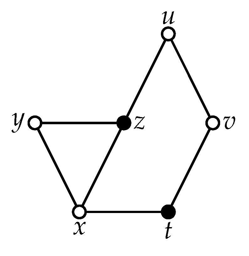We can immediately bound $\xi \left(T\right)$ as it is shown next. A tree T shown in Figure 2 has two strong supports u and w and one weak support v.

Theorem 3.

Let $k,\ell ,r,q$ be non-negative integers. Let T be a tree different from a path having k strong supports $v_1,\dots ,v_k$ and ℓ light supports. If $T-\{v_1,\dots ,v_k\}$ contains r components with at least one light support of T and q components with at least two light supports of T, then

$$k+q\le \xi \left(T\right)\le k+\ell -r.$$

Proof. 

Every maximal shortest path in a tree is a path between two leaves. Let S and L be the sets of strong and light supports of T, respectively. Further let $L^{\prime }$ be a set obtained from L by deleting one light support from every component of $T-S$ that contains a light support. Let x and y be arbitrary leaves. The $x,y$-geodesic P in T contains at least one support. Moreover, if the number of supports on P is exactly one then x and y correspond to the same strong support. Hence, the set $S\cup L^{\prime }$ covers P when P contains exactly one (strong) support. Similarly, P is covered by $S\cup L^{\prime }$ when P contains at least one strong support. So suppose that $V\left(P\right)\cap S=\varnothing$. Now P contains at least two light supports, which means that both light supports are in the same component of $T-S$ and at least one of them is in $L^{\prime }$. Hence, P is again covered by $S\cup L^{\prime }$ and the upper bound follows.

Let now D be a $\xi \left(T\right)$ set. Let v be a strong support vertex of T. Let $P_1$ and $P_2$ be two path components of $T-v$ and let ${\ell }_1$ and ${\ell }_2$ be leaves of T that correspond to v and belong to $P_1$ and $P_2$, respectively. Path P in T that starts at ${\ell }_1$ and ends at ${\ell }_2$ is a maximal shortest path containing exactly one vertex of degree three, namely v. As D is a $\xi \left(T\right)$ set, there exists a vertex from D that belongs to P. Hence, for every strong support vertex we have at least one vertex in D. Moreover, as follows from the previous analysis and the definition of strong supports, these vertices are pairwise different. Let $D^{\prime }$ be set obtained from D by deleting all vertices that correspond to strong support vertices. Now, let us consider an arbitrary component of $T-S$ that contains at least two light supports, say u and v. Let x and y be the leaves that correspond to u and v, respectively. Evidently, no vertex from $D-D^{\prime }$ lies on the $x,y$-geodesic. Hence, for every component of $T-S$ with at least two light supports we need at least one additional vertex in $D^{\prime }$. Hence, $\xi \left(t\right)\ge k+q$ and we are done.  □

Last theorem immediately implies the result for trees without light supports.

Corollary 3.

If T is a tree with $k>0$ strong supports and without light supports, then $\xi \left(T\right)=k$.

Let T be a tree. By $T^{-}$ we denote the forest of paths obtained from T by deleting all vertices of degree at least three. Let v be a strong support of T. The star neighborhood of v, denoted by $S{N}_T\left(v\right)$, contains v and all the vertices belonging to path components of $T^{-}$ that containins a neighbor of v in T.

Let $v_1$ be a leaf of T that corresponds to a strong support u. We order $V\left(T\right)$ by BFS algorithm that starts at $v_1$. In addition, we adjust BFS algorithm in such a way that for a vertex x it remembers also its closest ancestor (with respect to the constructed order) of degree more than two whenever such an ancestor exists and keeps it in $a\left(x\right)$. When such an ancestor does not exist, for all the vertices on the $v_1,u$-geodesic we set $a\left(x\right)=u$ for $x\ne u$ and $a\left(u\right)=v_1$. Hence, after the completion of the run of the designed algorithm, each variable $a(\ell )$, associated with a leaf ℓ, possesses the reference to the corresponding support of ℓ. Those vertices that appear more than once among the values $a(\ell )$, ℓ is any leaf, are strong supports and those which appear only once are light supports.

Now, let us restrict our attention to all the vertices of T of degree at least three accompanied with $v_1$. For these vertices reverse the order constructed by the enhanced BFS algorithm. We put them in list A together with information whether they are strong or light supports or no supports at all. This can be achieved with two Boolean functions $s\left(x\right)$ and $\ell \left(x\right)$ where $s\left(x\right)=1$ means that x is a strong support and $\ell \left(x\right)=1$ that x is a light support. If $s\left(x\right)=0=\ell \left(x\right)$, then x is not a support vertex. Moreover, the state $s\left(x\right)=1$ means that $\ell \left(x\right)=0$ and vice versa. Clearly, A ends with $v_1$.

Let x be the first vertex from A and $T^{\prime }=T-S{N}_T\left(x\right)$. If T contains more than one vertex of degree three, then $T^{\prime }$ is a tree and exactly one of the following cases occurs:

(a)

$a\left(x\right)$ is a strong support of T with $\mathrm{deg}\left(a\right(x\left)\right)>3$ and it is a strong support of $T^{\prime }$ as well;

(b)

$a\left(x\right)$ is a light or strong support of T with $\mathrm{deg}\left(a\right(x\left)\right)=3$ and is a vertex of degree two in $T^{\prime }$ — the later case occurs only when T has exactly two vertices of degree at least three;

(c)

$a\left(x\right)$ is a light support of T with $\mathrm{deg}\left(a\right(x\left)\right)>3$ and is a light support of $T^{\prime }$ as well;

(d)

$a\left(x\right)$ is not a support of T and is not a support of $T^{\prime }$.

In particular, (b) means that the ancestor of y of degree at least three that is closest to $a\left(x\right)$ in $T^{\prime }$, i.e., $y=a\left(a\right(x\left)\right)$ if it exists, either becomes a light support (providing y was not a support vertex of T) or becomes a strong support (whenever y was a support of T). In the special case, when T has exactly two vertices of degree at least three and one of them, say u, that is closer to $v_1$, has degree three, then $T^{\prime }$ is a path. It is also worth to mention that in the case (d) the vertex $a\left(x\right)$ has degree two in $T^{\prime }$ providing $\mathrm{deg}\left(a\right(x\left)\right)=3$ in T. Therefore, in such a case one needs to delete $a\left(x\right)$ from A (see the first condition in if sentence in the line 6 of Algorithm 1).

For an arbitrary tree T the value $\xi \left(T\right)$ and the corresponding $\xi \left(T\right)$ set D are computed in the main loop of Algorithm 1. The loop is repeated while A is not empty and, in addition, in every step we adjust the parameters $s\left(a\right(a\left(x\right)\left)\right),\ell \left(a\right(a\left(x\right)\left)\right)$ and $a\left(x\right)$ when needed. If the processed vertex satisfies the conditions described in the cases (a), (c) or (d), then nothing needs to be done (except, as it is explained above, for case (d) and $\mathrm{deg}\left(a\right(x\left)\right)=3$). If we have the case (b), then $a\left(x\right)$ is a vertex of degree two in $T^{\prime }$ and we change the value $a\left(x\right)$ to $a\left(a\right(x\left)\right)$ in the leaf t that corresponds to $a\left(x\right)$ in T, i.e., $a\left(t\right)=a\left(a\right(x\left)\right)$ after this operation. However, one can avoid this and just adopt the status of $a\left(a\right(x\left)\right)$ directly, see if sentences in lines 9–11 and 12–14 of Algorithm 1 for this.

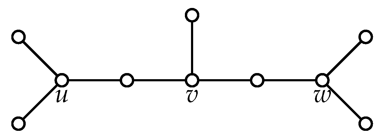
Algorithm 1: Computing $\xi \left(T\right)$ of a tree T.

We need to consider also the second condition in if sentence of line 6 of Algorithm 1. If $a\left(x\right)=v_1$, then $v_1$ corresponds to x and all maximal shortest paths that starts at $v_1$ contain x. Therefore, we delete $v_1$ from A. However, it is possible that $v_1$ corresponds to $a\left(x\right)$, where $a\left(x\right)$ is a strong support of T with exactly two leaves corresponding to $a\left(x\right)$. This means that the maximal shortest path between $v_1$ and the other leaf that corresponds to $a\left(x\right)$ is not covered yet. In such a case $v_1$ remains in A and it is added to D in the last step of the algorithm. Since $v_1$ belongs to A, Algorithm 1 works correctly also for paths.

Next we prove the correctness and estimate the time complexity of Algorithm 1.

Theorem 4.

Algorithm 1 correctly computes $\xi \left(T\right)$ and $\xi \left(T\right)$ set D for any tree T in $O\left(n\right)$ time where $n=\left|V\right(T\left)\right|$.

Proof. 

Let T be a tree and let $S=\{u_1,\dots ,u_k\}$ be all strong support vertices of T ordered by BFS algorithm starting from a leaf $v_1$ (the ordering is arbitrary but fixed). We prove the correctness of Algorithm 1 by induction on the number ℓ of light support vertices of T.

Let first $\ell =0$. We prove the basis again by induction on the number k of strong supports of T. If T has also no strong supports, then $T\cong P_r$ and the output of Algorithm 1 is $z=1$ and $D=\left\{v_1\right\}$ which is correct. If T has exactly one vertex of degree at least three, then T is a generalized star and we have $\xi \left(T\right)=1$ and $D=\left\{u_1\right\}$ by Theorem 2. The same result is obtained by Algorithm 1, because line 5 is executed exactly once and $v_1$ is deleted from A in line 7.

Let now $k>1$ and let $T^{\prime }=T-S{N}_T\left(u_k\right)$. As there are no light support vertices in T, we have, by (a), (b) and (d) no new supports in $T^{\prime }$. Hence, $T^{\prime }$ has at most $k-1$ strong supports (and no light supports) and Algorithm 1 correctly computes $\xi \left(T^{\prime }\right)$ and $\xi \left(T^{\prime }\right)$ set $D^{\prime }$. It is not hard to see, that $D^{\prime }=S-\left\{u_k\right\}$ when $\mathrm{deg}\left(u_1\right)>3$ and $D^{\prime }=(S-\{u_1,u_k\})\cup \left\{v_1\right\}$ when $\mathrm{deg}\left(u_1\right)=3$. By Corollary 3 we have $\xi \left(T^{\prime }\right)=k-1$ and $\xi \left(T\right)=k$. For T Algorithm 1 gives $z=\xi \left(T^{\prime }\right)+1=k$ and $D=D^{\prime }\cup \left\{u_k\right\}$. So, Algorithm 1 correctly computes $\xi \left(T\right)$ and $\xi \left(T\right)$ set D for a tree T without light supports.

Suppose now that T has $\ell \ge 1$ light supports and let w be the last light support in the fixed BFS order of T. By the assumption on input, $v_1$ corresponds to a strong support which is different from w. Let $u_{j_1},\dots ,u_{j_p}$ be all descendants of w that belong to S ordered by the fixed BFS ordering. For $T_0=T$ we define inductively $T_i=T_{i-1}-S{N}_{T_{i-1}}\left(u_{k-i+1}\right)$ for $i\in \{1,\dots ,k-j_1+1\}$. So, we end with $T_{k-j_1+1}$ and let $T^{\prime }=T_{k-j_1+1}$. At this stage $k-j_1+1$ strong supports were already processed by Algorithm 1, which means that $z=k-j_1+1$ and $D=\{u_{j_1},u_{j_1+1},\dots ,u_k\}$. In particular, notice that in the last step $a\left(u_{j_1}\right)=w$, ${\mathrm{deg}}_{T_{k-j_1}}\left(w\right)=3$ and the case (b) occurs for w. Hence, $T^{\prime }$ has one light support less than T and, by the induction hypothesis, Algorithm 1 correctly computes $\xi \left(T^{\prime }\right)$ and $\xi \left(T^{\prime }\right)$ set $D^{\prime }$. Therefore, at the end of the run of the algorithm we obtain $z=\xi \left(T^{\prime }\right)+k-j_1+1$ and $D=D^{\prime }\cup \{u_{j_1},u_{j_1+1},\dots ,u_k\}$.

It remains to show that $\xi \left(T\right)=z$ where D is a $\xi \left(T\right)$ set as $\left|D\right|=z$. For this notice that the path between two leaves x and y that belongs to some $T^{\prime }$ is covered by $D^{\prime }$ by induction hypothesis. Otherwise, a shortest path between x and y contains a strong support $u_s$ for some $s\in \{j_1,j_1+1,\dots ,k\}$ and is also covered by D. Hence, $\xi \left(T\right)\le z$. Conversely, we can show as in the proof of Theorem 3 that for every strong support $u_i$ there must be a vertex from a shortest path between two leaves corresponding to $u_i$ in every $\xi \left(T\right)$ set. So, if $\xi \left(T\right)<z$, then we have $|D_1\cap V\left(T^{\prime }\right)|<\xi \left(T^{\prime }\right)$ for a $\xi \left(T\right)$ set $D_1$. Thus $D_1\cap V\left(T^{\prime }\right)$ is not a $\xi \left(T^{\prime }\right)$ set and there exist two leaves x and y of $T^{\prime }$ such that the $x,y$-geodesic P is not covered by $D_1\cap V\left(T^{\prime }\right)$. But then P is not covered by $D_1$ in T, a contradiction. Therefore, $\xi \left(T\right)\ge z$ and the equality follows.

For the time complexity notice that adjusted BFS algorithm can be computed in linear time $O\left(n\right)$. For every vertex of list A Algorithm 1 performs constant number of operations (three in line 6 and either one in line 7 or two in line 10 or one in line 13). As there are less then n vertices in A the time complexity is linear.  □

The previous theorem enable us to show that the maximal shortest paths cover number of an (induced) subgraph can exceed the maximal shortest paths cover number of the original graph, that is $\xi \left(G\right)$ is not monotone with respect to taking neither subgraphs nor induced subgraphs (see [16,17]). A tree T is a caterpillar if the path $P_k$, called the spine, remains after deleting all leaves from T. Let $t_1,\dots ,t_k$ be non negative integers where $t_1,t_k>0$. We denote by $CT{P}_k(t_1,\dots ,t_k)$ the caterpillar with the spine $P_k$ and $t_i$ leaves attached to the i-th vertex of the spine for $i\in \{1,\dots ,k\}$. A caterpillar $CT{P}_k(2,0,1,0,2)$ is depicted in Figure 2.

Corollary 4.

The parameter $\xi \left(G\right)$ is not monotone neither with respect to taking subgraphs nor to taking induced subgraphs.

Proof. 

We have $\xi (P_q\square P_r)=2$ by Corollary 1. However, the caterpillar $CT{P}_q(2,2,\dots ,2)$ is a subgraph of the graph $P_q\square P_r$ when $r\ge 3$ and we have $\xi \left(CT{P}_q(2,2,\dots ,2)\right)=q$ by Theorem 4. Similarly, $CT{P}_q(2,0,2,0,\dots ,0,2)$ is an induced subgraph of $P_q\square P_r$ for an odd q and, according to Theorem 4, we have $\xi \left(CT{P}_q(2,0,2,0,\dots ,0,2)\right)=\frac{q+1}{2}$.  □

The result on tress allows us to describe also the relationship of $\xi \left(G\right)$ to the invariant k-path vertex cover number ${\psi }_k\left(G\right)$. By Proposition 4 we already have $\xi \left(G\right)\le \beta \left(G\right)={\psi }_2\left(G\right)$. However, this inequality cannot be extended for higher values of k.

Proposition 6.

If C is a positive constant and $k\ge 4$ an integer, then

(i) 

there exists a graph G with ${\psi }_k\left(G\right)-\xi \left(G\right)>C$;

(ii) 

there exists a graph G with $\xi \left(G\right)-{\psi }_k\left(G\right)>C$.

Proof. 

For the first statement it is sufficient to consider the path $P_n$ for sufficiently large n. We have already shown by Proposition 2 that $\xi \left(P_n\right)=1$ and by [10] we have ${\psi }_k\left(P_n\right)=\lfloor \frac{n}{k}\rfloor$.

For the second statement consider the caterpillar $G\cong CT{P}_n(2,2,\dots ,2)$ of order $3n$. The maximal shortest paths cover of G is formed by n vertices of spine by Theorem 4 and we have $\xi \left(G\right)=n$. On the hand ${\psi }_k\left(G\right)\le \lfloor \frac{n}{2}\rfloor$ whenever $k\ge 4$. This means $\xi \left(G\right)-{\psi }_k\left(G\right)\ge n-\lfloor \frac{n}{2}\rfloor \ge n-\frac{n}{2}=\frac{n}{2}$ and for sufficiently large n we obtain the desired result.  □

Notice that the first item of the above proposition holds also for $k\in \{2,3\}$. The example $G\cong CT{P}_n(2,0,2,\dots ,0,2)$ for an odd n shows that equality $\xi \left(G\right)={\psi }_3\left(G\right)$ is attainable. In contrast we have $\xi \left(K_r\right)=r-1>r-2={\psi }_3\left(K_3\right)$. Clearly, the inequality $\xi \left(G\right)>{\psi }_2\left(G\right)$ is not attainable, by Proposition 3, for a connected graph G as ${\psi }_2\left(G\right)=\beta \left(G\right)$.