Article

First Solution of Fractional Bioconvection with Power Law Kernel for a Vertical Surface

1
Department of Mathematics, University of Management and Technology Lahore, Lahore 54770, Pakistan
2
Institute of IR 4.0, The National University of Malaysia, Bangi 43600, Selangor, Malaysia
3
Faculty of Engineering and Natural Sciences, Bahcesehir University, Istanbul 34349, Turkey
4
Department of Mathematics & Statistics, McMaster University, Hamilton, ON L8S 4K1, Canada
5
Center for Dynamics, Faculty of Mathematics, Technische Universitt Dresden, 01062 Dresden, Germany
*
Authors to whom correspondence should be addressed.
Mathematics 2021, 9(12), 1366; https://doi.org/10.3390/math9121366
Submission received: 6 February 2021 / Revised: 4 June 2021 / Accepted: 8 June 2021 / Published: 12 June 2021
(This article belongs to the Special Issue New Trends on Boundary Value Problems)

Abstract

:
The present study provides the heat transfer analysis of a viscous fluid in the presence of bioconvection with a Caputo fractional derivative. The unsteady governing equations are solved by Laplace after using a dimensional analysis approach subject to the given constraints on the boundary. The impact of physical parameters can be seen through a graphical illustration. It is observed that the maximum decline in bioconvection and velocity can be attained for smaller values of the fractional parameter. The fractional approach can be very helpful in controlling the boundary layers of the fluid properties for different values of time. Additionally, it is observed that the model obtained with generalized constitutive laws predicts better memory than the model obtained with artificial replacement. Further, these results are compared with the existing literature to verify the validity of the present results.

1. Introduction

The term bioconvection is characterized by hydrodynamic instability and patterns in suspensions of biased swimming microorganisms. The velocity and spatial range of fluid motions are typically considerably higher than those associated with the velocity and size of individual cells, resulting in rapid cell transfer and the formation of specialized cell concentration visualization patterns. Biotechnology has evolved to integrate new and diverse sciences in the early 21st century, as introduced by Platt [1]. A variety of researchers dedicate their resources to revealing bioconvection characteristics, like Khan et al. [2], who conducted their research on the dynamics of the Cattaneo–Christov theory of heat and mass flow with bioconvection Oldroyd-B nanofluid. Assessment of bioconvection in Maxwell nanofluid equipped with nonlinear radiation using a Riga surface was carried out by Ramesh et al. [3]. Tlili et al. [4] previewed the analysis of micropolar nanofluid flow with partial slip and double stratification in MHD gyrotactic microorganisms. Heat production due to gyrotactic microorganisms with the bioconvection of a magnetohydrodynamic flow of nanofluid was examined by Khotha et al. [5]. Khan et al. [6] studied the entropy generation of bioconvection nanofluid streamlines between two spinning extendable discs. Shah et al. [7] investigated the microstructure and inertial properties of Maxwell base fluid stream-dependent magnetohydrodynamic suspended SWCNTs and MWCNTs with bioconvection and a vertical permeable cone. Research was conducted on the implications of activation energy, MHD, and bioconvection in the flow to the extended surface of third grade (non-Newtonian) fluid by Chu et al. [8]. Bhatti et al. [9] investigated the swimming of motile gyrotactic microorganisms and nanoparticles in blood flow with anisotropically tapered arteries. In that work, they discussed a theoretical study on the swimming of migratory gyrotactic microorganisms in a non-Newtonian blood-based nanofluid through an anisotropically narrowed artery.
Abbasi et al. [10] investigated the convective stream across a convective spinning stretching disc of viscoelastic nanofluid. With Maxwell, MHD, activation power, heat transfer, and Oldroyd-B on an extendable sheet, and also with a vertical rotating cylinder, the significance of bioconvection was studied by Waqas et al. [11,12]. The significance of various slips with gyrotactic motile microorganisms in the bioconvection stream of cross nanofluid over a wedge was studied. The value of viscoelastic nanofluid through a magnetic dipole and several slips on a cross nanofluid bioconvection stream past a wedge through gyrotactic motile microorganisms has been numerically examined by Alshomrani et al. [13,14]. A bioconvection study of third-grade nanofluid in von-Kármán flow with motile microorganisms was conducted by Ullah et al. [15]. The effectiveness of magnetohydrodynamic span and Carreau nanofluid has been established in entropy production details and gyrotactic motile microorganisms with transformations of von Neumann similarity by Naz et al. [16,17]. Alqarni et al. [18] investigated the transferred heat of micropolar nanofluid bioconvection flow through motile microorganisms and velocity slip conditions. Bioconvection with activation energy and Wu’s slip of magnetized couple stress nanofluid was studied by Khan et al. [19]. Sajid et al. [20] considered the effects of double-diffusive convection and motile microorganisms on tangent hyperbolic base fluid bioconvection MHD. A simulation of finite elements of bioconvection and superior-Fick diffusion effects over a vertically extending layer on micropolar-based nanofluid flow was discussed by Ali et al. [21]. The Newtonian heating effect on a time mixed convection nanofluid microorganism stream through the stagnation realm of an impulsively spinning sphere was examined by Mahdy et al. [22]. The effects of energy on Eyring’s motile microorganism-containing nanofluid on MHD flow were studied by Sharif et al. [23]. A computational simulation by coupled quasiliberalization magnetohydrodynamic bioconvective Casson nanofluid flow was carried out by Ansari et al. [24].
Fractional calculus is a field of mathematics used for the integration and differentiation of real or complex numbers. Even although calculus is historic, it has still gained attention in recent decades. Recently, mathematical simulations of heat transfer fluids, which play an important role in manufacturing, have also been studied by researchers, with significant applications. Usually, these simulations are expressed in standard integer-order partial differential equations. Note that the conventional PDEs cannot decipher the dynamical behavior of physical flow parameters and retention effects. To remove these defects, researchers focused on the fractional dynamic systems of heat transfer in simple and complex fluid models. Recently, many researchers have worked on the application of fractional calculus but they have not considered the unsteady effect of bioconvection in those heat transfer models. The wide range of fractional models, and their applications in applied sciences, can be seen in the following references [25,26,27,28,29,30,31,32,33,34,35,36,37,38,39,40,41,42,43,44].
The most interesting feature of the fractional operators is that there are several such operators. This helps researchers to select the most appropriate operator to characterize the implications of real global crises. Jarad et al. [45] modified fractional derivatives and Laplace transformed them. Vieru et al. [46] applied a Caputo fractional derivative to heat and mass transfer flow over a flat plate. They used the Laplace transform method to find exact solutions. They did not consider the bioconvection effect in their model. Abro et al. [47] investigated the thermal stability of Maxwell nanofluids by fractional derivatives with a singular kernel. Zhang et al. [48] analyzed a new mathematical model of COVID-19 through fractional derivatives of discrete and non-singular kernels. Rayal et al. [49] proposed a numerical analysis of a damped differential equation of an extended form associated with fractal–fractional derivatives through the use of the Lagrange wavelet fractional order. Singh et al. [50] presented a review of the chemical kinetics method of a fractional derivative of the Mittag-Leffler kernel form. Ghanbari et al. [51] studied new edge detection strategies focused on fractional derivatives of non-local and semi kernels. Son et al. [52] researched the liberalization regulatory problem with a granular neutrosophic fractional differential equation. Gambo et al. [53] discussed the unique nature of fractional differential equation solutions within the context of simplified Caputo fractional derivatives. Akgul et al. [54] analyzed the formulation of linear and nonlinear differential equations through simplified fractional derivatives. El-Nabulsi et al. [55] investigated results that were used to explore some novel aspects of fractional quantum field theory and many interesting consequences were revealed, in particular the complex quantum field theory, Dirac operators and the novel notion of mass without mass. El-Nabulsi et al. [56] studied the fractional field theory with Saxena–Kumbhat fractional integrals, fractional derivatives of order α , β and dynamical fractional integral exponents. Moshrefi et al. [57] analyzed the physical and geometrical interpretation of fractional operators. Cloot et al. [58] investigated the generalized groundwater flow equation using the concept of non-integer order derivatives. Lima et al. [59] studied the experimental signal analysis of robot impacts from a fractional calculus perspective. Bhalekar et al. [60] investigated the fractional Bloch equation with delay. In that work, they described the fractional Bloch equation with both fading memory and delay included. Odzijewicz et al. [61] invented variations of fractional calculus in the expression of a generalized fractional integral with physics applications. In that work, they investigated speculated fractional integrals with Lagrangian depending on classical derivatives, generalized fractional derivatives and integrals. Malinowska [62] studied the fractional variational calculus for non differentiable functions. Kulish et al. [63] investigated the application of fractional calculus to fluid mechanics. In that work, they examined the application of fractional calculus and of arbitrary differentiation to the solution of time-dependent, viscous diffusion fluid mechanics problems. Together with the Laplace transform method, the application of fractional calculus to the classical transient viscous diffusion equation in a semi-infinite space was shown to yield explicit analytical fractional solutions for the shear stress and fluid speed anywhere in the domain. El-Nabulsi et al. [64] investigated the path integral formulation of fractionally perturbed Lagrangian oscillators on a fractal. Meerschaert et al. [65] studied multidimensional advection and fractional dispersion. In that work, they found that the extension of the fractional diffusion equation to two or three dimensions is not as simple as an extension of the second order equation.
Vieru el al.’s [46] heat and mass transfer model is used in the absence of the bioconvection effect. After that, Shah et al. [25] studied analytical solutions for time-fractional boundary layer flow of viscous fluid over a vertical heat transfer surface including Caputo and Caputo–Fabrizio derivatives. Exact solutions were obtained through the Laplace transform method without the bioconvection effect.
The studies above were carried out with or without fractional derivatives in the absence of fractional bioconvection. On the other hand, the main task is to combine these two attractive topics, bioconvection and fractional derivatives. In the abovementioned literature, there is no single study of bioconvection with a Caputo fractional derivative. The theoretical model of heat transfer of fluid flow in the presence of bioconvection is solved with the Laplace transform method. A graphical discussion of flow parameters is presented through graphics.

2. Mathematical Formulation

Let us consider an unsteady heat transfer flow of a viscous fluid over a flat surface in an x y -coordinate system situated at y = 0 . In the beginning, at t = 0 , the plate and the fluid are at rest with reference surface temperature T and reference concentration of microorganisms N . After some time, the plate begins to move at a constant velocity and the surface temperature T w and the concentration of microorganisms of the plate N w increase. Since the plate has infinite length, every physical quantity is the function of y and t only and shown in Figure 1.
The momentum and bioconvection equations can be seen in limiting form in [66,67,68,69]
ρ u t ( y , t ) = μ u y y ( y , t ) + g ρ β T ( T T ) γ ( ρ m ρ ) ( N N ) ,
while the heat equation is
ρ C p T t ( y , t ) = k T y y ( y , t ) ,
and the unsteady bioconvection equation can be found in [66,67,68,69],
N t ( y , t ) = D n N y y ( y , t ) ,
subject to initial and boundary conditions
u ( y , 0 ) = 0 , T ( y , 0 ) = T , N ( y , 0 ) = N , for all y 0 ,
u ( 0 , t ) = u 0 H ( t ) , T ( 0 , t ) = T w , N ( 0 , t ) = N w , t > 0 ,
u ( y , t ) 0 , T ( y , t ) T , N ( y , t ) N , y , t > 0 .
We introduce the non-dimensional variables
y * = u 0 y ν , u * = u u 0 , t * = t u 0 2 ν , θ = T T T W T , N * = N N N W N , q * = q q o , J * = J J o ,
into Equations (1)–(6) and ignore the ( ) notation
u t ( y , t ) = u y y ( y , t ) + Gr [ θ ( y , t ) Ra N ( y , t ) ] ,
θ t ( y , t ) = 1 Pr θ y y ( y , t ) ,
N t ( y , t ) = 1 Lb N y y ( y , t ) ,
with dimensionless conditions
u ( y , 0 ) = 0 , θ ( y , 0 ) = 0 , N ( y , 0 ) = 0 ,
u ( 0 , t ) = H ( t ) , θ ( 0 , t ) = 1 , N ( 0 , t ) = 1 ,
u ( y , t ) 0 , θ ( y , t ) 0 , N ( y , t ) 0 , as y ,
where H ( t ) is the unit step function, Gr is the Grashof number, Gr = g ν β T ( T w T ) u 0 3 , Pr is the Prandtl number, Pr = ρ C p k , Lb = ν D N is the bioconvection Lewis number and Ra = γ ( ρ m ρ ) ( N w N ) β T ( T w T ) ρ is the bioconvection Rayleigh number.

3. The Solution of the Problem with Classical Time Derivative

This section deals with the solution of the temperature and velocity field with and without a fractional derivative and the Laplace transform method.

3.1. The Solution of Bioconvection

In this section, the solution of bioconvection given in Equation (10) and subject to boundary conditions (11)–(13) by the assistance of the Laplace transform strategy can be obtained in the following way:
s N ¯ ( y , s ) = 1 L b N ¯ y y ( y , s ) ,
while associated conditions in the transformed domain are:
N ¯ ( 0 , s ) = 1 s , N ¯ ( y , s ) 0 , as y .
The general solution of Equation (14) under condition (15):
N ¯ ( y , s ) = 1 s e y Lb s ,
is found by applying the inverse Laplace to Equation (16)
N ( y , t ) = erfc y Lb 2 t ,
where erfc ( . ) is Gauss’s complementary error function.

3.2. The Solution of Temperature Field

In this section, the solution of energy in Equation (9) is subject to the boundary conditions (11)–(13) with the assistance of the Laplace transform method and is given as
s θ ¯ ( y , s ) = 1 Pr θ ¯ y y ( y , s ) ,
with associated conditions:
θ ¯ ( 0 , s ) = 1 s , θ ¯ ( y , s ) , 0 , as y .
The solution of Equation (18) is subject to the conditions given in (19), so we have
θ ¯ ( y , s ) = 1 s e y Pr s ,
with its inverse Laplace transform form
θ ( y , t ) = erfc y Pr 2 t ,
where erfc ( . ) is Gauss’s complementary error function.

3.3. The Solution of the Velocity Field

This section deals with the solution of momentum in Equation (8) subject to the boundary conditions (11)–(13) through the assistance of the Laplace transform technique and the procedure is given below:
s u ¯ ( y , s ) = u ¯ y y ( y , s ) + Gr [ θ ¯ ( y , s ) Ra N ¯ ( y , s ) ] ,
and relevant boundary conditions in transform domain are:
u ¯ ( y , s ) = 1 s , u ¯ ( y , s ) 0 , as y .
A general solution of Equation (22) subject to the constraints given in (23):
u ¯ ( y , s ) = e y s s + Gr Pr 1 e y s s 2 e y Pr s s 2 RaGr Lb 1 e y s s 2 e y Lb s s 2 .
Taking the inverse Laplace of Equation (24) with the help of the following formula given in [25,46] gives:
L 1 1 s 2 e y a s = t + a y 2 2 e r f c y a 2 t y a t π e a y 2 4 t
u ( y , t ) = e r f c y 2 t + Gr Pr 1 t + y 2 2 e r f c y 2 t y t π e y 2 4 t Gr Pr 1 t + Pr y 2 2 e r f c y Pr 2 t y Pr t π e Pr y 2 4 t RaGr Lb 1 t + y 2 2 e r f c y 2 t y t π e y 2 4 t + RaGr Lb 1 t + Lb y 2 2 e r f c y Lb 2 t y Lb t π e Lb y 2 4 t .
Equation (25) is valid only for Pr 1 and Lb 1 .

3.4. Fractional Modeling

In the literature presented in the Introduction, researchers addressed bioconvection with classical time derivatives or the steady case, either analytically or numerically, in the absence of a fractional derivative approach. Usually, these models are represented in terms of traditional integer-order partial differential equations (PDEs). However, traditional PDEs cannot decode the complex behavior of physical flow parameters and memory effects. The classical calculus measures the instant rate of change of the output when the input level changes. Therefore, it is not able to include the previous state of the system, called the memory effect. In fractional calculus (FC), the rate of change is affected by all points of the considered interval, so it is able to incorporate the previous history/memory effects of any system. The order of the fractional derivative is treated as an index of memory. Therefore, we considered the present fractional model. Further, in the fractional derivative approach in convective problems, scientists have ignored the bioconvection effect. Therefore, our main target was to combine these two branches in order to cover the gap which is still not reported in the existing literature. For this purpose, we generalized the ordinary model with fractional derivatives and found analytical solutions of fractional energy equations and fractional bioconvection. There are two method for fractional modeling in the existing literature and: (i) we develop the fractional model of governing equations by replacing the integer order with non-integer order derivative, (ii) we develop the fractional model for energy balance equations and bioconvection through generalized constitutive relations and use these solutions in a classical momentum equation to obtain an analytical solution for the velocity field.

3.5. Solution of the Fractional Model Using Generalized Constitutive Relations

Firstly, we develop the constitutive fractional model for energy balance equations and bioconvection equations and solve them with the Laplace transform method, followed by the velocity field. The momentum equation for viscous fluid containing the bioconvection term is given by
ρ u ( y , t ) t = τ ( y , t ) y + g ρ β T ( T T ) γ ( ρ m ρ ) ( N N ) .
The constitutive equation is
τ ( y , t ) = μ u ( y , t ) y .
The equation of thermal balance is
( ρ C p ) T ( y , t ) t = q ( y , t ) y .
By Fourier’s law, the thermal flux equation of heat conduction is
q ( y , t ) = k T ( y , t ) t .
The equation of diffusion balance is
N ( y , t ) t = J ( y , t ) y .
The equation of bioconvection concentration is
J ( y , t ) = D n N ( y , t ) y .
By introducing the dimensionless variables from Equation (7) into (26)–(31), we have the momentum equation containing the bioconvection term, given by
u ( y , t ) t = c o τ ( y , t ) y + Gr θ ( y , t ) Ra N ( y , t ) .
The constitutive equation is
τ ( y , t ) = c 1 u ( y , t ) y .
The equation of thermal balance is
θ ( y , t ) t = c 2 q ( y , t ) y .
By Fourier’s law, the thermal flux equation of heat conduction is
q ( y , t ) = c 3 θ ( y , t ) t .
The equation of diffusion balance is
N ( y , t ) t = c 4 J ( y , t ) y .
The equation of bioconvection concentration is
J ( y , t ) = c 5 N ( y , t ) y .
By using Equation (33) in Equation (32), we have the momentum equation in dimensionless form:
u ( y , t ) t = u 2 ( y , t ) y 2 + Gr θ ( y , t ) Ra N ( y , t ) .
where c o = τ o ρ u o 2 , c 1 = ρ u o 2 τ o , c 2 = q o ρ C p ( T w T , c 3 = k u o ( T w T ) q o ν , c 4 = J o u o ( N w N ) , c 5 = D n u o ( N w N ) J o ν .
Hristov [70] and Povstenko [71] found the constitutive thermal flux equation with the generalized Fourier’s law:
Q ( y , t ) = b 1 β C D t 1 β θ ( y , t ) y , 0 < β 1 ,
and the constitutive equation for bioconvection balance equation:
J ( y , t ) = c 1 γ C D t 1 γ N ( y , t ) y , 0 < γ 1 .
In the equations above, C D t β or C D t γ is the Caputo time fractional operator defined in [46].
By introducing Equations (39) and (40) into Equations (34) and (36), respectively, we have. In [72,73] the authors used the same kind of fractional modeling for some heat transfer models.
θ ( y , t ) t = c 2 b 1 β C D t 1 β θ ( y , t ) y y ,
N ( y , t ) t = c 4 c 1 γ C D t 1 γ N ( y , t ) y y .
In order to get the equivalent forms of Equations (41) and (42), we apply left inverse operators I t 1 β ( . ) and I t 1 γ ( . ) and on both sides we have
C D t β θ ( y , t ) = c 6 2 θ ( y , t ) y 2 ,
C D t γ N ( y , t ) = c 7 2 N ( y , t ) y 2 .
The solution of Equation (43) is subject to conditions given in Equation (19) by means of the Laplace transform method
θ ¯ ( y , s ) = 1 s e x p y s β c 6 ,
written in a suitable form,
θ ( y , s ) = 1 s + i = 1 ( y c 6 ) i i ! s 1 β i 2 .
By taking the inverse Laplace transform of Equation (46), we have
θ ( y , t ) = 1 + i = 1 ( y c 6 ) i t β i / 2 i ! Γ ( 1 β i ) .
Therefore, by following a similar procedure, the solution of bioconvection can be obtained as follows:
N ( y , t ) = 1 + j = 1 ( y c 7 ) j t γ j / 2 j ! Γ ( 1 η j ) .
In order to obtain the analytical solutions for momentum equation, we use the expressions of energy and bioconvection of fractional order in momentum Equation (38) after applying the Laplace transform subject to conditions (23), we have
u ( y , s ) = e y s s + Gr ( s β 1 c 6 ) 1 e y s s 2 e y s β c 6 s 2 GrRa ( s γ 1 c 7 ) 1 e y s s 2 e y s γ c 7 s 2 .
In order to obtain the inverse Laplace transform analytically, Equation (49) can be written in its suitable form
u ¯ ( y , s ) = 1 s + i = 1 ( y ) i i ! s 1 i 2 + Gr j = 0 k = 0 ( c 6 ) j + 1 ( y ) k k ! s 1 + β j + β j k 2 Gr j = 0 l = 0 ( c 6 ) j + 1 l 2 ( y ) l l ! s 1 + β j + β j β l 2 GrRa m = 0 n = 0 ( c 7 ) m + 1 ( y ) n n ! s 1 + β m + β m n 2 + GrRa m = 0 p = 0 ( c 7 ) m + 1 p 2 ( y ) p p ! s 1 + β m + β m β p 2 .
Taking the inverse Laplace of Equation (50), we have
u ( y , t ) = 1 + i = 1 ( y ) i t i 2 i ! Γ ( 1 i 2 ) + Gr j = 0 k = 0 ( c 6 ) j + 1 ( y ) k t β j j k 2 k ! Γ ( 1 + β j + β j k 2 ) Gr j = 0 l = 0 ( c 6 ) j + 1 l 2 ( y ) l t β j + β j β l 2 l ! Γ ( 1 + β j + β j β l 2 ) GrRa m = 0 n = 0 ( c 7 ) m + 1 ( y ) n t β m m n 2 n ! Γ ( 1 + β m + β m n 2 ) + GrRa m = 0 p = 0 ( c 7 ) m + 1 p 2 ( y ) p t β m + β m β p 2 p ! Γ ( 1 + β m + β m β p 2 ) .

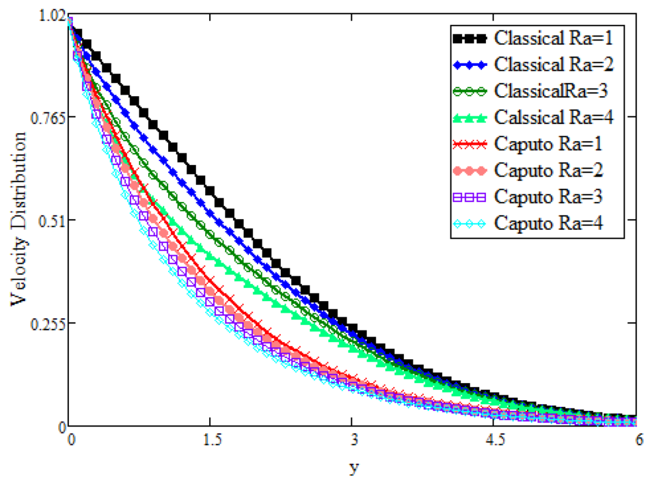
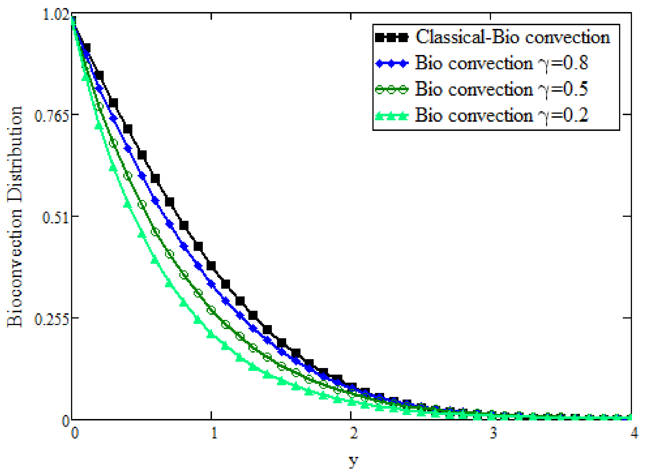
4. Results and Discussion

The unsteady bioconvection effect is studied in this investigation with a fractional derivative for a vertical surface. By the Laplace transform method, exact solutions are obtained and presented in the form of Wright’s function. Some graphs are plotted to see the physical impact of flow parameters and are presented in this section. Figure 2 shows the comparison between the Caputo fractional and classical velocity field by keeping other parameters constant. It is clear from the figure that for α = 0.95 the fluid velocity shows decay and for α = 0.6 more decay is detected. Additionally, for α = 0.4 and α = 0.2 , the velocity field reaches the maximum decline. This fact explains the memory effect of the present fractional operator for varying values of the fractional parameter. The Caputo fractional explains the memory of the function and further shows dual behavior for long and short times due to the power law kernel that appears in its definition. Such results are very important in some experimental data. Hence, by using a fractional approach, the velocity exhibits more memory than the classical approach.
Figure 3 presents the outcome of the bioconvection Rayleigh number Ra and the comparison between the Caputo fractional and classical approach to variable velocity field was carried out by keeping other parameters constant. It is clear from the figure that the fluid velocity falls when increasing the values of bioconvection Rayleigh number Ra . This is due to the fact that, for larger values of Ra , the buoyancy effect from the transportation of microorganisms decreases. Moreover, fractional velocity exhibits a greater decline than the classical approach.
In Figure 4, the same behavior Pr can be observed for the velocity with integer and non-integer orders. From the figure, it is clear that velocity is a decreasing function of Pr . Physically, Pr is the dimensionless number that tests the relative breadth of a boundary layer of thermal conductivity and momentum. With higher values of Pr , thermal conductivity is reduced, the viscosity of the fluid is enhanced and, finally, a decline in velocity is observed. It is also observed that the boundary layer breadth declines.
Figure 5 presents increasing values of the time and shows that velocity can be enhanced for longer periods of time. Figure 6 shows a comparison between Caputo and classical Grashof number ( Gr ) in the field variable velocity field, by keeping other parameters constant, and an opposite trend of Pr can be seen. It is observed that field variable fluid velocity can be enhanced for larger values of the Grashof number ( Gr ). These phenomena occur with increases in the velocity due to the increased thermal buoyancy effect. Figure 7 shows bioconvection when keeping other parameters constant and varying the values of the Caputo fractional parameter α , and it is observed that bioconvection shows a decline for larger values of α and the maximum decline can be attained for smaller values of α near the plate. It is also found that the momentum boundary layer thickness decreases.
Figure 8 shows the evaluation among Caputo fractional and classical bioconvection fields by keeping other parameters constant, and it is shown that the bioconvection field can be decreased with higher values of Lb . This is because Lb is reciprocal to mass diffusivity, so its large values decrease the bioconvection profile. Figure 9 is plotted for the validation of the present results. In the absence of bioconvection, the present result was reduced to the result obtained in [25] and they are clearly in good agreement. Further, in order to justify the present fractional modeling with a classical time derivative, we created a fractional model with artificial replacement of the integer order derivative with a non-integer order and a fractional model obtained with generalized constitutive laws and found very interesting results, which are presented in Figure 10, Figure 11 and Figure 12. In the literature, many results are obtained with artificial replacement after making the governing equation dimensionless. Here, we present a comparison between the fractional modeling obtained with artificial replacement and generalized constitutive laws for temperature, bioconvection and velocity field. It is clear from the figures that artificial replacement exhibits memory, but not accurately, as the correct fractional approach through constitutive laws does. In addition, a correct mathematical model obtained with generalized laws shows a rapid decline in the boundary layers of the fluid properties.

5. Conclusions

The present study deals with bioconvection with a heat transfer model with a Caputo fractional model. The exact solutions are obtained for the dimensionless governing equations with Laplace transform methods. Some physical impacts of flow parameters have been discussed through graphical illustrations. The major outcomes are the following:
  • The fractional parameter can be used to control the boundary layers of the fluid properties like bioconvection, temperature and velocity.
  • The fractional approach can be the best fit in some experimental work, where the needed and desired results can be achieved for different values of fractional parameters and time.
  • The fractional model obtained with generalized constitutive laws gives better and more accurate results in terms of memory than the fractional approach with artificial replacement.
  • The present results are compared with the existing literature in the absence of bioconvection and they are in good agreement.

Author Contributions

Formal analysis, S.U.R.; Investigation, A.A.; Methodology, A.A.; Resources, M.S.; Supervision, S.S.; Visualization, M.I.A.; Writing original draft, M.I.A. and S.U.R. All authors have read and agreed to the published version of the manuscript.

Funding

This research received no external funding.

Institutional Review Board Statement

Not applicable.

Informed Consent Statement

Not applicable.

Acknowledgments

The authors are greatly appreciative and indebted to the University of Management and Technology, Lahore, Pakistan for facilitating and supporting the study effort.

Conflicts of Interest

The authors declare no conflict of interest.

Abbreviations

The following abbreviations are used in this manuscript:
SymbolName
ρ Fluid density
sLaplace transform
μ Viscosity
Pr Prandtl number
gGravitational acceleration
Lb Bioconvection Lewis number
TFluid temperature
Gr Grashof number
T w Temperature at wall
Ra Bioconvection Rayleigh number
T Ambient temperature of the fluid
erfc ( . ) Gauss’s error function of complimentary
β T Volumetric coefficient of thermal expansion
ϕ The dimensionless nanoparticle volume fraction
ρ m Mass density
tTime (s)
ρ Fluid density
N * Concentration of microorganisms
NThe dimensionless concentration of microorganisms
N The density of motile microorganisms
C p Specific heat at constant pressure
kThermal conductivity
D N Diffusivity of microorganisms
θ Dimensionless temperature
uVelocity

References

  1. Platt, J.R. Bioconvection patterns in cultures of free-swimming organisms. Science 1961, 133, 1766–1767. [Google Scholar] [CrossRef] [PubMed]
  2. Khan, N.S.; Shah, Q.; Sohail, A. Dynamics with Cattaneo-Christov heat and mass flux theory of bioconvection Oldroyd-B nanofluid. Adv. Mech. Eng. 2020, 12, 1–20. [Google Scholar]
  3. Ramesh, K.; Khan, S.U.; Jameel, M.; Khan, M.I.; Chu, Y.-M.; Kadry, S. Bioconvection assessment in Maxwell nanofluid configured by a Riga surface with nonlinear thermal radiation and activation energy. Surf. Interfaces 2020, 21, 100749. [Google Scholar] [CrossRef]
  4. Tlili, I.; Ramzan, M.; Nisa, H.U.; Shutaywi, M.; Shah, Z.; Kumam, P. Onset of gyrotactic microorganisms in MHD micropolar nanofluid flow with partial slip and double stratification. J. King Saud Univ. Sci. 2020, 32, 2741–2751. [Google Scholar] [CrossRef]
  5. Kotha, G.; Kolipaula, V.R.; Rao, M.V.S.; Penki, S.; Chamkha, A.J. Internal heat generation on bioconvection of an MHD nanofluid flow due to gyrotactic microorganisms. Eur. J. Plus 2020, 135, 1–19. [Google Scholar]
  6. Khan, N.S.; Shah, Q.; Bhaumik, A.; Kumam, P.; Thounthong, P.; Amiri, I. Entropy generation in bioconvection nanofluid flow between two stretchable rotating disks. Sci. Rep. 2020, 10, 4448. [Google Scholar] [CrossRef]
  7. Shah, Z.; Alzahrani, E.; Jawad, M.; Khan, U. Microstructure and inertial characteristics of MHD suspended SWCNTS and MWCNTS based Maxwell nanofluid flow with bioconvection and entropy generation past a permeable vertical cone. Coatings 2020, 10, 998. [Google Scholar] [CrossRef]
  8. Chu, Y.-M.; Khan, M.I.; Khan, N.B.; Kadry, S.; Khan, S.U.; Tlili, I.; Nayak, M. Significance of activation energy, bio-convection and magnetohydrodynamic in flow of third grade fluid (non-Newtonian) towards stretched surface: A Buongiorno model analysis. Int. Heat Mass Transf. 2020, 118, 104893. [Google Scholar] [CrossRef]
  9. Bhatti, M.M.; Marin, M.; Zeeshan, A.; Ellahi, R.; Abdelsalam, S.I. Swimming of motile gyrotactic microorganisms and nanoparticles in blood flow through anisotropically tapered arteries. Front. Phys. 2020, 8, 95. [Google Scholar] [CrossRef] [Green Version]
  10. Abbasi, A.; Mabood, F.; Farooq, W.; Batool, M. Bioconvective flow of viscoelastic nanofluid over a convective rotating stretching disk. Int. Commun. Heat Mass Transf. 2020, 119, 104921. [Google Scholar] [CrossRef]
  11. Waqas, H.; Khan, S.A.; Khan, S.U.; Khan, M.I.; Kadry, S.; Chu, Y.M. Falkner-skan time-dependent bioconvrction flow of cross nanofluid with nonlinear thermal radiation, activation energy and melting process. Int. Commun. Heat Mass Transf. 2021, 120, 105028. [Google Scholar] [CrossRef]
  12. Waqas, H.; Imran, M.; Bhatti, M. Influence of bioconvection on Maxwell nanofluid flow with the swimming of motile microorganisms over a vertical rotating cylinder. Chin. J. Phys. 2020, 68, 558–577. [Google Scholar] [CrossRef]
  13. Alshomrani, A.S.; Ullah, M.Z.; Baleanu, D. Importance of multiple slips on bioconvection flow of cross nanofluid past a wedge with gyrotactic motile microorganisms. Case Stud. Therm. Eng. 2020, 22, 100798. [Google Scholar] [CrossRef]
  14. Alshomrani, A.S. Numerical investigation for bio-convection flow of viscoelastic nanofluid with magnetic dipole and motile microorganisms. Arab. J. Sci. Eng. 2021, 46, 5945–5956. [Google Scholar] [CrossRef]
  15. Ullah, M.Z.; Jang, T. An efficient numerical scheme for analyzing bioconvection in vonk LarmLan flow of third-grade nanofluid with motile microorganisms. Alex. Eng. J. 2020, 59, 2739–2752. [Google Scholar] [CrossRef]
  16. Naz, R.; Noor, M.; Hayat, T.; Javed, M.; Alsaedi, A. Dynamism of magnetohydrodynamic cross nanofluid with particulars of entropy generation and gyrotactic motile microorganisms. Int. Commun. Heat Mass Transf. 2020, 110, 104431. [Google Scholar] [CrossRef]
  17. Naz, R.; Tariq, S.; Sohail, M.; Shah, Z. Investigation of entropy generation in stratified MHD Carreau nanofluid with gyrotactic microorganisms under Von Neumann similarity transformations. Eur. Phys. J. Plus 2020, 135, 178. [Google Scholar] [CrossRef]
  18. Alqarni, M.; Waqas, H.; Imran, M.; Alghamdi, M.; Muhammad, T. Thermal transport of bioconvection flow of micropolar nanofluid with motile microorganisms and velocity slip effects. Phys. Scr. 2020, 96, 015220. [Google Scholar] [CrossRef]
  19. Khan, S.U.; Waqas, H.; Bhatti, M.; Imran, M. Bioconvection in the rheology of magnetized couple stress nanofluid featuring activation energy and wufs slip. J. Non-Equilib. Thermodyn. 2020, 45, 81–95. [Google Scholar] [CrossRef]
  20. Sajid, T.; Sagheer, M.; Hussain, S.; Shahzad, F. Impact of double-diffusive convection and motile gyrotactic microorganisms on magnetohydrodynamics bioconvection tangent hyperbolic nanofluid. Open Phys. 2020, 18, 74–88. [Google Scholar] [CrossRef]
  21. Ali, B.; Hussain, S.; Nie, Y.; Ali, L.; Hassan, S.U. Finite element simulation of bioconvection and Cattaneo-Christov effects on micropolar based nanofluid flow over a vertically stretching sheet. Chin. J. Phys. 2020, 68, 654–670. [Google Scholar] [CrossRef]
  22. Mahdy, A.; Nabwey, H.A. Microorganisms time-mixed convection nanofluid flow by the stagnation domain of an impulsively rotating sphere due to newtonian heating. Results Phys. 2020, 19, 103347. [Google Scholar] [CrossRef]
  23. Sharif, H.; Naeem, M.N.; Khadimallah, M.A.; Ayed, H.; Bouzgarrou, S.M.; Naim, A.F.A.; Hussain, S.; Hussain, M.; Iqbal, Z.; Tounsi, A. Energy effects on mhd flow of eyringfs nanofluid containing motile microorganism. Adv. Concr. Constr. 2020, 10, 357–367. [Google Scholar]
  24. Ansari, M.S.; Otegbeye, O.; Trivedi, M.; Goqo, S. Magnetohydrodynamic bioconvective Casson nanofluid flow: A numerical simulation by paired quasilinearisationh. J. Appl. Comput. Mech. 2020. [Google Scholar] [CrossRef]
  25. Shah, N.A.; Imran, M.A.; Miraj, F. Exact solutions of time fractional free convection flows of viscous fluid over an isothermal vertical plate with Caputo and Caputo-fabrizio derivatives. J. Prime Res. Math. 2017, 13, 56–74. [Google Scholar]
  26. Podlubny, I. Fractional Differential Equations: An Introduction to Fractional Derivatives, Fractional Differential Equations, to Methods of Their Solution and Some of Their Applications; Elsevier: Edinburgh, UK, 1998. [Google Scholar]
  27. Samko, S.G.; Kilbas, A.A.; Marichev Oleg, I. Fractional Integrals and Derivatives; Gordon and Breach Science Publishers: London, UK, 1993. [Google Scholar]
  28. Kilbas, A. Theory and Applications of Fractional Differential Equations; Elsevier Science Inc.: New York, NY, USA, 2006; ISBN 978-0-444-51832-3. [Google Scholar]
  29. Magin, R.L. Fractional Calculus in Bioengineering; Begell House Redding: Redding, CT, USA, 2006; Volume 2. [Google Scholar]
  30. Caputo, M.; Fabrizio, M. Applications of new time and spatial fractional derivatives with exponential kernels. Progr. Fract. Differ. Appl. 2016, 2, 1–11. [Google Scholar] [CrossRef]
  31. Hilfer, R. Applications of Fractional Calculus in Physics; World Scientific: Singapore, 2000. [Google Scholar]
  32. Lorenzo, C.F.; Hartley, T.T. Variable order and distributed order fractional operators. Nonlinear Dyn. 2002, 29, 57–98. [Google Scholar] [CrossRef]
  33. Salahshour, S.; Ahmadian, A.; Senu, N.; Baleanu, D.; Agarwal, P. On analytical solutions of the fractional differential equation with uncertainty: Application to the basset problem. Entropy 2015, 17, 885–902. [Google Scholar] [CrossRef] [Green Version]
  34. Pakdaman, M.; Ahmadian, A.; Effati, S.; Salahshour, S.; Baleanu, D. Solving differential equations of fractional order using an optimization technique based on training artificial neural network. Appl. Math. Comput. 2017, 293, 81–95. [Google Scholar] [CrossRef]
  35. Ahmadian, A.; Salahshour, S.; Chan, C.S. Fractional differential systems: A fuzzy solution based on operational matrix of shifted Chebyshev polynomials and its applications. IEEE Trans. Fuzzy Syst. 2016, 25, 218–236. [Google Scholar] [CrossRef]
  36. Ahmadian, A.; Ismail, F.; Salahshour, S.; Baleanu, D.; Ghaemi, F. Uncertain viscoelastic models with fractional order: A new spectral tau method to study the numerical simulations of the solution. Commun. Nonlinear Sci. Numer. Simul. 2017, 53, 44–64. [Google Scholar] [CrossRef]
  37. Shahriyar, M.; Ismail, F.; Aghabeigi, S.; Ahmadian, A.; Salahshour, S. An eigenvalueeigenvector method for solving a system of fractional differential equations with uncertainty. Math. Probl. Eng. 2013, 2013, 579761. [Google Scholar] [CrossRef]
  38. Salahshour, S.; Ahmadian, A.; Abbasbandy, S.; Baleanu, D. M-fractional derivative under interval uncertainty: Theory, properties and applications. Chaos Solitons Fractals 2018, 117, 84–93. [Google Scholar] [CrossRef]
  39. Basit, A.; Imran, M.A.; Akgul, A. Convective flow of a fractional second grade fluid containing different nanoparticles with Prabhakar fractional derivative subject to non-uniform velocity at the boundary. Math. Meth. Appl. Sci. 2021. [Google Scholar] [CrossRef]
  40. Butt, A.R.; Abdullah, M.; Raza, N.; Imran, M.A. Influence of non-integer order parameter and Hartmann number on the heat and mass transfer flow of a Jeffery fluid over an oscillating vertical plate via Caputo-Fabrizio time fractional derivatives. Eur. Phys. J. Plus 2017, 132, 414. [Google Scholar] [CrossRef]
  41. Jamil, M.; Khan, N.A.; Imran, M.A. New exact solutions for an Oldroyd-B Fluid with Fractional Derivatives: Stokes’ first problem. Int. J. Nonlinear Sci. Numer. Simul. 2013, 14, 443–451. [Google Scholar] [CrossRef]
  42. Asjad, M.I.; Aleem, M.; Ahmadian, A.; Salahshour, S.; Ferrara, M. New trends of fractional modeling and heat and mass transfer investigation of (SWCNTs and MWCNTs)-CMC based nanofluids flow over inclined plate with generalized boundary conditions. Chin. J. Phys. 2020, 66, 497–516. [Google Scholar] [CrossRef]
  43. Ahmad, M.M.; Imran, M.A.; Aleem, M.; Khan, I. A comparative study and analysis of natural convection flow of MHD non-Newtonian fluid in the presence of heat source and first-order chemical reaction. J. Therm. Anal. Calorim. 2019, 137, 1783–1796. [Google Scholar] [CrossRef]
  44. Sohail, A.; Vieru, D.; Imran, M.A. Influence of side walls on the oscillating motion of a Maxwell fluid over an infinite plate. Mechanics 2013, 19, 269–276. [Google Scholar] [CrossRef]
  45. Jarad, F.; Abdeljawad, T. Generalized fractional derivatives and laplace transform. Discret. Contin. Dyn. Syst. S 2020, 13, 709–722. [Google Scholar] [CrossRef] [Green Version]
  46. Vieru, D.; Fetecau, C.; Fetecau, C. Time-fractional free convection flow near a vertical plate with Newtonian heating and mass diffusion. Therm. Sci. 2015, 19 (Suppl. 1), 85–98. [Google Scholar] [CrossRef]
  47. Abro, K.A.; Soomro, M.; Atangana, A.; Lomez-Aguilar, J.G. Thermophysical properties of Maxwell nanofluids via fractional derivatives with regular kernel. J. Therm. Anal. Calorim. 2020, 1–11. [Google Scholar] [CrossRef]
  48. Zhang, Z. A novel covid-19 mathematical model with fractional derivatives: Singular and nonsingular kernels. Chaos Solitons Fractals 2020, 139, 110060. [Google Scholar] [CrossRef]
  49. Rayal, A.; Verma, S.R. Numerical analysis of pantograph differential equation of the stretched type associated with fractal-fractional derivatives via fractional order Legendre wavelets. Chaos Solitons Fractals 2020, 139, 110076. [Google Scholar] [CrossRef]
  50. Singh, J.; Kumar, D.; Baleanu, D. On the analysis of chemical kinetics system pertaining to a fractional derivative with Mittag-Leffler type kernel. Chaos Interdiscip. J. Nonlinear Sci. 2017, 27, 103113. [Google Scholar] [CrossRef] [PubMed]
  51. Ghanbari, B.; Atangana, A. Some new edge detecting techniques based on fractional derivatives with non-local and non-singular kernels. Adv. Differ. Equ. 2020, 2020, 1–19. [Google Scholar] [CrossRef]
  52. Son, N.T.; Dong, N.P.; Long, H.V.; Khastan, A. Linear quadratic regulator problem governed by granular neutrosophic fractional differential equations. ISA Trans. 2020, 97, 296–316. [Google Scholar] [CrossRef] [PubMed]
  53. Gambo, Y.; Ameen, R.; Jarad, F.; Abdeljawad, T. Existence and uniqueness of solutions to fractional differential equations in the frame of generalized Caputo fractional derivatives. Adv. Differ. Equ. 2018, 2018, 134. [Google Scholar] [CrossRef] [Green Version]
  54. Akgul, E.K. Solutions of the linear and nonlinear differential equations within the generalized fractional derivatives. Chaos Interdiscip. J. Nonlinear Sci. 2019, 29, 023108. [Google Scholar] [CrossRef]
  55. El-Nabulsi, A.R. Complexified quantum field theory and hmass without massh from multidimensional fractional actionlike variational approach with dynamical fractional exponents. Chaos Solitons Fractals 2009, 42, 2384–2398. [Google Scholar] [CrossRef]
  56. El-Nabulsi, A.; Wu, C. Fractional complexified field theory from saxena-kumbhat fractional integral, fractional derivative of order and dynamical fractional integral exponent. Afr. Diaspora J. Math. New Ser. 2012, 13, 45–61. [Google Scholar]
  57. Moshrefi-Torbati, M.; Hammond, J. Physical and geometrical interpretation of fractional operators. J. Frankl. Inst. 1998, 335, 1077–1086. [Google Scholar] [CrossRef]
  58. Cloot, A.; Botha, J. A generalised groundwater flow equation using the concept of noninteger order derivatives. Water Sa 2006, 32, 1–7. [Google Scholar]
  59. Lima, M.F.; Machado, J.T.; CrisLostomo, M. Experimental signal analysis of robot impacts in a fractional calculus perspective. J. Adv. Comput. Intell. Intell. Inform. 2007, 11, 1079–1085. [Google Scholar] [CrossRef]
  60. Bhalekar, S.; Daftardar-Gejji, V.; Baleanu, D.; Magin, R. Fractional bloch equation with delay. Comput. Math. Appl. 2011, 61, 1355–1365. [Google Scholar] [CrossRef] [Green Version]
  61. Odzijewicz, T.; Malinowska, A.B.; Torres, D.F. Fractional calculus of variations in terms of a generalized fractional integral with applications to physics. Abstr. Appl. Anal. 2012, 2012, 871912. [Google Scholar] [CrossRef] [Green Version]
  62. Malinowska, A.B. Fractional variational calculus for non-differentiable functions. In Fractional Dynamics and Control; Springer: New York, NY, USA, 2012; pp. 97–108. [Google Scholar]
  63. Kulish, V.V.; Lage, J.L. Application of fractional calculus to fluid mechanics. J. Fluids Eng. 2002, 124, 803–806. [Google Scholar] [CrossRef]
  64. El-Nabulsi, R.A. Path integral formulation of fractionally perturbed Lagrangian oscillators on fractal. J. Stat. Phys. 2018, 172, 1617–1640. [Google Scholar] [CrossRef]
  65. Meerschaert, M.M.; Benson, D.A.; Bäumer, B. Multidimensional advection and fractional dispersion. Phys. Rev. E 1999, 59, 5026. [Google Scholar] [CrossRef] [Green Version]
  66. Raees, A.; Xu, H.; Liao, S.-J. Unsteady mixed nano-bioconvection flow in a horizontal channel with its upper plate expanding or contracting. Int. J. Heat Mass Transf. 2015, 86, 174–182. [Google Scholar] [CrossRef]
  67. Zhao, Q.; Xu, H.; Tao, L. Unsteady bioconvection squeezing flow in a horizontal channel with chemical reaction and magnetic field effects. Math. Probl. Eng. 2017, 2017, 2541413. [Google Scholar] [CrossRef]
  68. Latiff, N.A.A.; Uddin, M.J.; Leg, O.A.B.; Ismail, A.I. Unsteady forced bioconvection slip flow of a micropolar nanofluid from a stretching/shrinking sheet. Proc. Inst. Mech. Eng. Part N J. Nanomater. Nanoeng. Nanosyst. 2016, 230, 177–187. [Google Scholar]
  69. Ali, L.; Liu, X.; Ali, B.; Mujeed, S.; Abdal, S. Finite element simulation of multi-slip effects on unsteady MHD bioconvective micropolar nanofluid flow over a sheet with solutal and thermal convective boundary conditions. Coatings 2019, 9, 842. [Google Scholar] [CrossRef]
  70. Hristov, J. Derivatives with non-singular kernels from the Caputo-Fabrizio definition and beyond: Appraising analysis with emphasis on diffusion models. Front. Fract. Calc. 2017, 1, 270–342. [Google Scholar]
  71. Povstenko, Y. Fractional Thermoelasticity; Springer: Cham, Switzerland, 2015. [Google Scholar]
  72. Ahmed, N.; Vieru, D.; Fetecau, C.; Shah, N.A. Convective flows of generalized time-nonlocal nanofluids through a vertical rectangular channel. Phys. Fluids 2018, 30, 052002. [Google Scholar] [CrossRef]
  73. Shah, N.A.; Khan, I.; Aleem, M.; Asjad, M.I. Influence of magnetic field on double convection problem of fractional viscous fluid over an exponentially moving vertical plate: New trends of caputo time-fractional derivative model. Adv. Mech. Eng. 2019, 11. [Google Scholar] [CrossRef] [Green Version]
Figure 1. Geometry of the problem.
Mathematics 09 01366 g001
Figure 2. Comparative analysis of velocity distribution for different β and γ values.
Mathematics 09 01366 g002
Figure 3. Comparative analysis of velocity distribution for different Ra values.
Mathematics 09 01366 g003
Figure 4. Comparative analysis of velocity distribution for different Pr values.
Mathematics 09 01366 g004
Figure 5. Comparative analysis of velocity distribution for different time values.
Mathematics 09 01366 g005
Figure 6. Comparative analysis of velocity distribution for different Gr values.
Mathematics 09 01366 g006
Figure 7. Comparative analysis of bioconvection distribution for different γ values.
Mathematics 09 01366 g007
Figure 8. Comparative analysis of bioconvection distribution for different Lb values.
Mathematics 09 01366 g008
Figure 9. Comparison between present Results in the absence of bioconvection and Nehad el al. [25].
Mathematics 09 01366 g009
Figure 10. Comparison of temperature between classical time derivative, Caputo fractional model with artificial replacement and Caputo model with generalized constitutive law.
Mathematics 09 01366 g010
Figure 11. Comparison of bioconvection between classical time derivative, Caputo fractional model with artificial replacement and Caputo model with generalized constitutive law.
Mathematics 09 01366 g011
Figure 12. Comparison of velocity between classical time derivative, Caputo fractional model with artificial replacement and Caputo model with generalized constitutive law.
Mathematics 09 01366 g012
Publisher’s Note: MDPI stays neutral with regard to jurisdictional claims in published maps and institutional affiliations.

