Article

Distributed State Estimation Based Distributed Model Predictive Control

1
Liaoning Province Key Laboratory of Control Technology for Chemical Processes, Shenyang University of Chemical Technology, Shenyang 110142, China
2
Department of Chemical & Materials Engineering, University of Alberta, Edmonton, AB T6G 1H9, Canada
*
Author to whom correspondence should be addressed.
Mathematics 2021, 9(12), 1327; https://doi.org/10.3390/math9121327
Submission received: 24 April 2021 / Revised: 30 May 2021 / Accepted: 3 June 2021 / Published: 9 June 2021
(This article belongs to the Special Issue Mathematics and Engineering II)

Abstract

:
In this work, we consider output-feedback distributed model predictive control (DMPC) based on distributed state estimation with bounded process disturbances and output measurement noise. Specifically, a state estimation scheme based on observer-enhanced distributed moving horizon estimation (DMHE) is considered for distributed state estimation purposes. The observer-enhanced DMHE ensures that the state estimates of the system reach a small neighborhood of the actual state values quickly and then maintain within the neighborhood. This implies that the estimation error is bounded. Based on the state estimates provided by the DMHE, a DMPC algorithm is developed based on Lyapunov techniques. In the proposed design, the DMHE and the DMPC are evaluated synchronously every sampling time. The proposed output DMPC is applied to a simulated chemical process and the simulation results show the applicability and effectiveness of the proposed distributed estimation and control approach.

1. Introduction

In modern industry, large-scale complex processes with distributed structure and dynamic coupling characteristics exist widely, such as large-scale petrochemical processes, wastewater treatment plants, and so forth. These complex processes usually consist of multiple operating units (subsystems) that are connected tightly through materials, energy and information flows. The decentralized control in general does not fully consider the interaction between the subsystems, which typically leads to reduced plant-wide control performance due to the lack of coordination and cooperation between the subsystem controllers. While the centralized control structure provides potentially the best performance, it is not favorable from the computational and fault tolerance view points. In the past decade, with the advances of information technology, distributed control system (in particular, distributed model predictive control (DMPC)) has received significant attention and development. DMPC has been widely recognized as the control framework for the next-generation complex processes [1,2,3,4,5,6].
In the design of DMPC algorithms, the real-time state information of a system is needed. It is in general difficult to install sufficient sensors to measure all the states. State estimation techniques should be used to estimate the state every sampling time. State estimation takes advantage of the system model, noise characteristics, real-time output measurement to reconstruct the actual state of the system. In a distributed control system, a distributed state estimation scheme is preferred from a fault tolerance perspective. In the study of distributed state estimation, there are many distributed Kalman filtering research results [7,8]. These methods are mainly based on the consensus algorithm and have great limitation for nonlinear systems [9]. Distributed moving horizon estimation (DMHE) for linear constrained systems was presented in [10] and was extended to nonlinear system in [11]. However, these DMHE designs do not give bounded estimation error and the convergence speed is not tunable. These features make the above DMHE not suitable for output feedback control designs.
In [12], an observer-enhanced DMHE algorithm was presented. It is designed for output feedback control with bounded measurement and process noise. In this algorithm, the observer-enhanced MHE developed in [13] is adopted for the subsystem MHE design. For each subsystem MHE design, an auxiliary nonlinear high-gain observer is used to calculate a reference state estimate and the reference state estimate is then used to construct a confidence region for the actual state. The subsystem MHE is restricted to optimize the state estimate within the confidence region. This approach ensures that the estimation error is always bounded and the convergence speed can also be tuned by tuning the auxiliary observer. DMHE for nonlinear systems have also been discussed in [14,15,16,17,18].
The observer-enhanced MHE has been adopted to design control systems based on output feedback. In [19], a centralized MPC was designed based on the observer-enhanced MHE and a triggered implementation strategy was developed to reduce its computational load. In [20], an output feedback economic model predictive control was developed based on the observer-enhanced MHE. The above output feedback control methods were implemented within a centralized framework. DMPC has been widely considered as an indispensable advanced control technology to realize intelligent manufacturing and smart power grid [21,22]. In the DMPC design, the subsystem MPCs coordinate and communicate to obtain the optimal control performance via the communication network. Relevant research results and reviews can be found in [1,2]. However, most of the existing DMPC designs assume that the states of the subsystems or the global system can be measured, which cannot be guaranteed in many applications.
Motivated by the above considerations, in the present work, we consider output-feedback distributed model predictive control (DMPC) based on distributed state estimation with bounded process disturbances and output measurement noise. Specifically, the observer-enhanced DMHE is adopted to obtain state estimates of the system. The observer-enhanced DMHE ensures that the state estimates of the system reach a small neighborhood of the actual state values quickly. Based on the state estimates provided by the DMHE, a DMPC algorithm designed using Lyapunov techniques is developed. In the proposed design, the DMHE and the DMPC are evaluated synchronously every sampling time. The proposed output DMPC is applied to a simulated chemical process and the simulation results show the applicability and effectiveness of the proposed distributed estimation and control approach.

2. Preliminaries

2.1. Notation and Definitions

In this work, | · | represents the Euclidean norm of a scalar or a vector. For each x 1 and x 2 in a given region of x, if there exists a positive constant L f x such that | f ( x 1 ) f ( x 2 ) | L f x | x 1 x 2 | , the function f ( x ) is said to be locally Lipschitz with respect to its argument x. The pseudoinverse of a matrix (or vector) A is denoted by A + . x T denotes the transpose of vector x. In the set of I = { 1 , , m } , m denotes the total number of subsystems. The symbol d i a g ( w ) is a diagonal matrix whose diagonal elements are every element of vector w. Finally, the operator ‘×’ denotes the Cartesian product: Ω 1 × Ω 2 = { ( x 1 , x 2 ) : x 1 Ω 1 and x 2 Ω 2 } .

2.2. System Description

In this paper, it is assumed that a class of nonlinear systems are composed of m interconnected subsystems. In particular, the state-space model of the i-th subsystem can be described as follows:
x ˙ i ( t ) = f i ( x i ( t ) , u i ( t ) , w i ( t ) ) + f ˜ i ( X i ( t ) ) , y i ( t ) = h i ( x i ( t ) , u i ( t ) ) + v i ( t ) ,
where x i ( t ) R n x i denotes the state variables of subsystem i, u i ( t ) R n u i represents the control input of subsystem i and y i ( t ) R n y i denotes the measurement output of the ith subsystem. w i ( t ) R n w i represents the disturbances and v i ( t ) R n v i characterizes the measurement noise of the ith subsystem. f ˜ i ( X i ( t ) ) represents the interaction between subsystem i and other subsystems, the state vector X i ( t ) R n X i contains subsystem states involved in the above interaction. The sets I i I ( i I ) represents the set of subsystem indices whose subsystem state variables are involved in X i and the set I i ( i I ) is assumed to be known in this work.
It is assumed that the control input of the ith subsystem is restricted in a nonempty convex set U i R n u i , i I :
U i : = { u i R n u i : | u i | u i m a x } ,
where u i m a x is the maximum amplitude of the input constraint. For the subsystem i, it is assumed that the process disturbances and measurement noise are bounded such as w i W i and v i V i for all i I :
W i : = { w i R n w i : | w i | θ w i , θ w i 0 } , V i : = { v i R n v i : | v i | θ v i , θ v i 0 } ,
where θ w i , θ v i for i I are known positive real scalars. f i , f ˜ i and h i with i I are assumed locally Lipschitz of their arguments. The global system state vector x is denoted as x = [ x 1 T x i T x m T ] T R n x , the input vector and output vector are denoted as u = [ u 1 T u i T u m T ] T R n u and y = [ y 1 T y i T y m T ] T R n y respectively. The dynamics of the global nonlinear system are described as the following form:
x ˙ ( t ) = f ( x ( t ) , u ( t ) , w ( t ) ) + f ˜ ( x ( t ) ) , y ( t ) = h ( x ( t ) , u ( t ) ) + v ( t ) ,
where w ( t ) R n w denotes the disturbance vector composed by the subsystem disturbance vectors, and v ( t ) R n v is the corresponding global measurement noise vector. f, h and f ˜ are the corresponding compositions of f i , h i and f ˜ i , i I , respectively. It is assumed that f, h and f ˜ are locally Lipschitz of their arguments which satisfy the initial conditions f ( 0 , 0 , 0 ) = 0 , h ( 0 ) = 0 and f ˜ ( 0 ) = 0 .

2.3. Stabilizability Assumptions

In each subsystem, for all x l D l R n x l , l I i , where D l is a compact set which contains the origin, it is assumed that there exists a nonlinear state feedback controller u i = k i ( X i ) , which can render the origin of the nominal subsystem asymptotically stable in the case of satisfying the input constraints. This assumption implies that for each subsystem, there exists a control Lyapunov function V i ( x i ) which is continuous differentiable. Note that in the above assumption, it is assumed that the state feedback controller has access to both the state of subsystem i and the states of its neighboring subsystems that are needed to describe the interaction between subsystem i and other subsystems.

2.4. Observability Assumptions

We further assume that the ith subsystem is observable, for i I . For the nominal subsystem of Equation (1) without considering the interaction (i.e., f ˜ i ( X i ( t ) ) 0 for all t), a deterministic nonlinear observer can be designed as follows:
z ˙ i ( t ) = F i ( ϵ i , z i ( t ) , u i ( t ) , h ( x i ( t ) ) ) ,
where z i is the state vector of the ith subsystem observer, ϵ i denotes a positive tuning parameter for the convergence rate of the above observer. h ( x i ( t ) ) represents the noise-free output measurement of the subsystem i, i I . Equation (5) indicates that, for all t, if f ˜ i ( X i ( t ) ) 0 , w i ( t ) 0 , z i can asymptotically approach x i . This assumption further implies that there exists a KL function β i under this assumption such that:
| z i ( t ) x i ( t ) | β i ( | z i ( 0 ) x i ( 0 ) | , t ) ,
where z i ( 0 ) denotes the initial guess of the subsystem state and x i ( 0 ) is the subsystem’s initial state. It is also assumed that F i is locally Lipschitz, i I . A type of observer satisfying the above assumptions is a high-gain observer [23].

3. Distributed LMPC Based on Distributed State Estimation

In this section, the distributed Lyapunov model predictive control (LMPC) based on distributed state estimation is presented. For all subsystems, it is assumed that the measurement output vector of the ith subsystem y i ( i I ) is sampled periodically and synchronously such that t k = t 0 + k Δ , where t k denotes the time instant, t 0 = 0 represents the initial time, k is a positive integer and Δ denotes a fixed sampling interval. It is also assumed that the estimator of the subsystem i can directly and immediately access its local output measurement y i every sampling time. The LMPC of the i-th subsystem can communicate with the other neighboring subsystems through a shared communication network.

3.1. Implementation Algorithm

In the proposed approach, both the fast convergence rate of the nonlinear observer and the robustness of the observer-enhanced moving horizon estimation (MHE) to output measurement noise are considered. During a short period from the initial time, state estimation is performed using an augmented nonlinear observer based on F i for each subsystem i. The short period is described as t 0 t < t s w , where t 0 is the initial time, t s w is a multiples of the sampling time Δ . Due to the fast convergence of the nonlinear observer, the estimate of the subsystem state reaches a small neighborhood of the actual state value before time t s w . During this period, the augmented nonlinear observer of subsystem i is evaluated and it communicates with other subsystems l, l I i , continuously. Meanwhile, it provides state estimates to the LMPC of subsystem i ( L M P C i ) during this short period. Then from time instant t s w , after the subsystem state estimates have converged to a small neighborhood of the actual subsystem states, the estimator of each subsystem switches from the augmented nonlinear observer to MHE. The MHE of subsystem i ( M H E i ) is evaluated to provide the optimal estimate of the subsystem state to L M P C i for time t t s w . It is assumed that the distributed state estimators ( M H E i ) and the distributed LMPCs ( L M P C i ) are evaluated with the same sampling time Δ . The above described implementation strategy of the proposed distributed Lyapunov model predictive control based on distributed state estimation can be summarized as follows:
1.
At t 0 = 0 , the augmented nonlinear observer based on F i of each subsystem is initialized with the subsystem output measurement y i ( 0 ) and the initial subsystem state guess z i ( 0 ) , i I .
2.
At t k > 0 , if t k < t s w , go to Step 2.1; otherwise, go to Step 2.2.
2.1
The subsystem state estimate z i ( t ) , t [ t k 1 , t k ] , i I , is calculated continuously by the corresponding augmented nonlinear observer based on the output measurements of subsystem i, the output measurements and state estimates of its related subsystems l, l I i , received by subsystem i via communication network. The estimate result z i ( t k ) is sent to the corresponding L M P C i of subsystem i and go to Step 3.
2.2
The local M H E i of subsystem i estimates the current optimal subsystem state estimate x ^ i * ( t k ) , t [ t k 1 , t k ] , i I , based on current and previous output measurement y i ( t q ) of subsystem i with q = k N e , , k , the previous output measurements and subsystem state estimates y l ( t q ) and x l ( t q ) from subsystems l, l I i , with q = k N e , , k 1 , are sent to subsystem i via communication network, where N e is the horizon of the M H E i . The estimate x ^ i * ( t k ) , i I , is sent to the corresponding subsystem L M P C i and go to Step 3.
3.
Based on z i ( t ) or x ^ i * ( t k ) , i I , the L M P C i of subsystem i calculates the future input trajectory u i ( t ) for t [ t k , t k + N c ] , where N c denotes the prediction horizon of L M P C i . The first value of the input trajectory u i ( t k ) , i I , is applied to the system.
4.
Go to Step 2. ( k k + 1 ).

3.2. Subsystem Observer Design

In this paper, an augmented subsystem observer based on observer (5) for the ith subsystem is designed, i I . For each subsystem i, the estimates of the neighboring subsystem states X i are received via the communication network every sampling time. An approximation of the interaction between the ith subsystem and other subsystems that involved in set I i can be calculated by them. The subsystem observer is designed as follows:
z ˙ i ( t ) = F i ( ϵ i , z i ( t ) , u i ( t ) , y i ( t k 1 ) ) + f ˜ i ( Z i ( t k 1 ) ) + l I i K i , l z l ( t k 1 ) y l ( t k 1 ) h l ( z l ( t k 1 ) ) ,
where z i ( t ) is the state of the nonlinear observer, the interactions between the ith subsystem and other neighboring subsystems l, l I i are taken into account in this observer. Z i ( t k 1 ) and z l ( t k 1 ) are the state estimates of X i ( t k 1 ) and x l ( t k 1 ) calculated by observer respectively. The first term of the right-hand side of nonlinear observer (7) comes from Equation (5); the next term f ˜ i ( Z i ( t k 1 ) ) describes the interactions between the ith subsystem and other subsystems; the last term is a correction term based on actual measurement y l , l I i . In the last term, the gains K i , l z l ( t k 1 ) which are functions of z l ( t k 1 ) can be determined as follows:
K i , l z l ( t k 1 ) = f ˜ i x l h l x l + | z l ( t k 1 ) .
The correction gains in Equation (8) can be obtained by linear approximation via Taylor series expansion.

3.3. Subsystem Observer-Enhanced MHE

In this paper, a distributed observer-enhanced moving horizon estimation (distributed MHE) scheme developed in [12] is adopted. In every subsystem, the augmented nonlinear observer discussed in the earlier subsection is used to tune the convergence rate of the subsystem MHE. The nonlinear augmented observer which includes an error correction term calculates a subsystem reference state estimate first; then based on the reference state estimate, the local subsystem MHE determines a confidence region of the actual system state and optimizes the state estimate within the confidence region. At time instant t k , the local MHE for subsystem i can be described as follows:
min x ˜ i ( t k N e ) , , x ˜ i ( t k ) q = k N e k 1 | w i ( t q ) | Q i 1 2 + q = k N e k | v i ( t q ) | R i 1 2 + V i ( x ˜ i ( t k N e ) )
(9b) s.t. x ˜ ˙ i ( t ) = f i ( x ˜ i ( t ) , u i ( t q ) , w i ( t q ) ) + f ˜ i ( X ^ i ( t q ) ) , t [ t q , t q + 1 ] , q = k N e , , k 1 (9c) y i ( t q ) = h i ( x ˜ i ( t q ) , u i ( t q ) ) + v i ( t q ) , q = k N e , , k (9d) w i ( t q ) W i , v i ( t q ) V i , x ˜ i ( t q ) X i , u i ( t q ) U i , q = k N e , , k (9e) z ˙ n , i ( t ) = F i ( ϵ i , z n , i ( t ) , u i ( t ) , y i ( t k 1 ) ) + f ˜ i ( X ^ i * ( t k 1 ) ) ) + l I i K i , l x ^ l * ( t k 1 ) y l ( t k 1 ) h l ( x ^ l * ( t k 1 ) ) (9f) z n , i ( t k 1 ) = x ^ i * ( t k 1 ) (9g) K i , l x ^ l * ( t k 1 ) = f ˜ i x l h l x l + | x ^ l * ( t k 1 ) (9h) | x ˜ i ( t k ) z n , i ( t k ) | κ i | y i ( t k ) h i ( z n , i ( t k ) ) | .
In Equation (9), x ˜ i is the optimized estimation result; N e denotes the state estimation horizon; Q i is the covariance matrices of process disturbances w i ; R i is the covariance matrices of the measurement noise v i ; the arrival cost function is described by V i ( x ˜ i ( t k N e ) ) , which includes all the past information up to time t k N e . It is assumed that w i and v i are piece-wise constant variables with sampling time Δ to guarantee the above optimization problem is finite dimensional. Parameter κ i is a positive constant which depends on the properties of the corresponding subsystem.
Once the Equation (9) is solved, a series of subsystem states x ˜ i * ( t k N e ) , , x ˜ i * ( t k ) can be determined. The optimal subsystem state estimate denoted as x ^ i * ( t k ) is the last element x ˜ i * ( t k ) in the series:
x ^ i * ( t k ) = x ˜ i * ( t k ) .
In the subsystem observer-enhanced MHE scheme (9), (9a) is the cost function which needs to be minimized. Constraints (9b) and (9c) are subsystem model. (9d) denotes the constraint boundary of w i , v i and subsystem state x ˜ i . Constraints (9e)–(9h) are used to determine a confidence region. The confidence region is calculated based on the augmented nonlinear observer. Note that the observer (9e) embedded in MHE is evaluated based on the optimal state estimate x ^ i * of the previous time instant. (9h) describes the confidence region determined by the parameter κ i , the current subsystem output measurement y i ( t k ) and state estimate z n , i ( t k ) given by the nonlinear observer (9e).

3.4. Subsystem Lyapunov MPC

In the distributed Lyapunov MPC scheme, for each subsystem i, i I , the design of local LMPC is based on the subsystem nominal model and the subsystem state estimate. In the time interval 0 < t k < t s w , the state estimate z i ( t k ) is calculated by the observer F i ; when t k t s w , the optimal state estimate x ^ i * ( t k ) is obtained from the corresponding local MHE. In the remainder of this work, x ^ i is used to denote the state estimate of subsystem i for the consistency of expression. At time instant t k , the subsystem LMPC i optimizes its future control input sequence using its subsystem nominal model, it is assumed that the state trajectories of related subsystems keep the same as the values sent to subsystem i at the previous time instant t k 1 . Specifically, the LMPC i is based on the following optimization problem:
u i * ( τ | t k ) = a r g min u i ( τ ) S ( Δ ) t k t k + N c [ x ˜ i ( τ ) T Q i x ˜ i ( τ ) + u i ( τ ) T R i u i ( τ ) ] d τ
(11b) s.t. x ˜ ˙ i ( τ ) = f i ( x ˜ i ( τ ) , u i ( τ ) , 0 ) + f ˜ i ( X ˜ i ( τ ) ) (11c) x ˜ i ( t k ) = x ^ i ( t k ) , X ˜ i ( t k ) = X ^ i ( t k ) (11d) u i ( τ ) U i (11e) V i ( x ˜ i ( t k ) ) x ˜ i f i ( x ˜ i ( t k ) , u i ( t k ) , 0 ) + f ˜ i ( X ˜ i ( t k ) ) V i ( x ^ i ( t k ) ) x ^ i f i ( x ^ i ( t k ) , k i ( X ^ i ( t k ) ) , 0 ) + f ˜ i ( X ^ i ( t k ) ) ,
where u i * denotes the optimal input sequence of subsystem i calculated by the above optimization problem, S ( Δ ) means piece-wise constant function and Δ is the sampling period, N c denotes the prediction horizon, x ˜ i is the predicted state trajectory of the nominal subsystem i with control inputs calculated by the local LMPC, Q i and R i are positive definite weighting matrices.
In the local LMPC optimization problem (11), for subsystem i, i I , (11a) is the cost function concerning the subsystem state vector and input vector; (11b) is the subsystem nominal model comes from Equation (1); (11c) define the initial condition calculated by local MHE at time instant t k , including the state estimate x ^ i ( t k ) of subsystem i and its related subsystem state X ^ i ( t k ) obtained through communication network; (11d) denotes the constraint on control input sequence u i ; (11e) expresses the stability constraint based on Lyapunov function V i and the nonlinear controller k i ( X ^ i ( t k ) ) , 0 ) at time instant t k . The subsystem manipulated input under the control of the distributed MHE-LPMC is defined by the following expression:
u i ( t ) = u i * ( t | t k ) , t [ t k , t k + 1 ) , i I .

4. A Brief Stability Analysis

In this section, we provide a sketch of the stability analysis of the proposed distributed control scheme. The stability of the closed-loop system can be shown following similar arguments in our previous work in [12,20,24].
First, according to the results of [12], the estimation error provided by the adopted distributed observer-enhanced MHE is ultimately bounded in a small neighborhood of the origin when some conditions are satisfied. The detailed conditions can be found in [12]. In [12], it was also shown that the convergence speed of the distributed observer-enhanced MHE can be tuned by tuning the convergence speed of the reference observer. If high-gain observers are used to design the reference nonlinear observers, the convergence speed can be fast and the switching time t s w can be made to be small (for example, smaller than a sampling time Δ ).
Second, we consider the stability of each subsystem controller. Let us assume that the interactions between subsystems are constant or absent for now. Since the switching time t s w can be made to be small, the duration such that each local LMPC operates with a less accurate state estimate is small. As long as the operation in this small duration does not drive the subsystem state outside of the region of attraction, the subsystem stability can be ensure. This requires that the initial condition is not very close to the boundary of the region of attraction and that there is no finite-time escape phenomena in the subsystem dynamics. A detailed mathematical characterization of these conditions can be found in [20].
Third, the above explains how to analyze the stability of each subsystem without considering the interaction between subsystems. For a distributed control system, this is indeed important. To take into account the interaction, the approach used in [24] can be adopted. The information exchanged between the neighboring subsystems can be used to compensate for the interaction between the subsystems. A detailed characterization of the conditions needed can be derived following similar approach as in [24].

5. The Simulation Application

5.1. Chemical Process

In this paper, the proposed scheme is applied to a chemical process to verify its applicability. The process consists in two continuous stirred tank reactors (CSTRs) and a flash tank separator. Figure 1 shows a schematic diagram of the chemical process. There is a feed stream of pure reactant A goes into the first CSTR at flow rate F 10 and temperature T 10 . In the CSTR, two elementary reactions take place: A B , B C , where the reactant is A, the desired product and the side product are B and C, respectively. A recycle stream from the separator also goes into the first CSTR at flow rate F r and temperature T 3 . The effluent of the first CSTR enters the second CSTR at flow rate F 1 and temperate T 1 . Another feed stream of pure A at flow rate F 20 and temperature T 20 also goes into the second CSTR to generate more product. In the second CSTR, the same reactions as in the first CSTR occur. The outlet stream from the second CSTR goes into the flash separator at flow rate F 2 and temperature T 2 . In the separator, flash separation happens and the bottom outlet stream F 3 primarily contains the product. A portion of the top effluent is purged and the rest is recycled back to the first CSTR. Both reactors and the separator are equipped with a jacket for heat input or removal.
A detailed description of the process and a description of the dynamical model of the process can be found in [12]. In the dynamical model, the manipulated inputs are the heat inputs/removals, Q 1 , Q 2 and Q 3 . We can divide the whole system into three subsystems: the first CSTR, the second CSTR and the last flash separator. The subsystem states can be described as x i = [ x A i x B i T i ] T , i = 1 , 2 , 3 , where x A i and x B i are subsystem mass fractions of A and B, T i is the subsystem temperature. The entire system state is the aggregation of the three subsystem states as follows:
x = [ x A 1 x B 1 T 1 x A 2 x B 2 T 2 x A 3 x B 3 T 3 ] T ,
where temperatures T 1 , T 2 and T 3 are assumed to be measured and are sampled synchronously. The sampling time is Δ = 0.005   h = 18   s . The mass fractions of A i and B i , i = 1 , 2 , 3 , are unmeasurable and should be estimated.
The steady-state of the system state x s and the steady-state manipulated input Q s are shown in Table 1. The control objective is to steer the process from the initial state x 0 to the steady-state x s .

5.2. Observer and Controller Designs

The detailed modeling equations of the process can be found in [12]. By examining the modeling equations, it can be found that the dynamics of each subsystem i in the chemical process, i = 1 , 2 , 3 , can be described compactly in the following form:
x ˙ i ( t ) = f i ( X i ( t ) ) + g i ( X i ( t ) ) u i ( t ) y i ( t ) = C x i ( t ) ,
where x i = [ x i 1 x i 2 x i 3 ] T = [ x A i x B i T i ] T denotes the subsystem state vector, X i denotes the state vector containing all the neighboring subsystems’ states. The control input u i of subsystem i is the heat input Q i ( k J / h ), i = 1 , 2 , 3 .
It is assumed that the three temperatures are measured. The subsystem states are estimated based on the three temperature measurements. First, the nonlinear observer in Equation (7) is designed for each subsystem. For subsystem i, i = 1 , 2 , 3 , the first term on the right-hand side of Equation (7) is designed as follows:
z ˙ i ( t ) = f i ( z i ( t ) , 0 ) + d Φ i ( z i ) d z i 1 G o , i ( y i ( t ) h i ( z i ( t ) ) ) Φ i ( z i ) = [ h i ( z i ) , h i ( z i ) z i f i , h i z i f i z i f i ] G o , i = [ k o , i ( 1 ) / θ , k o , i ( 2 ) / θ 2 , k o , i ( 3 ) / θ 3 ] T ,
where z i is the state of nonlinear observer and G o , i is a gain vector. In the gain vector, θ sets to 0.5, and K o , i = [ k o , i ( 1 ) , k o , i ( 2 ) , k o , i ( 3 ) ] T is determined such that the eigenvalues of the matrix A o , i K o , i C o , i are placed at 1.1 , 1 and 1.2 , with A o i = [ 0 1 0 ; 0 0 1 ; 0 0 0 ] and C o , i = [ 1 0 0 ] . The second term (interaction model) and the third term (correction term) on the right-hand side of observer (7) are added to Equation (15) to finish the design of the augmented nonlinear observer for a subsystem. From the system model in [12], it can be seen that the states of subsystem 1 are affected by subsystem 3 only; therefore, I 1 ={3}. Similarly, it can be found that I 2 ={1}, I 3 ={2}. The gains K i , l , i I , l I i in the third term of observer (7) are determined following Equation (8) to be the following:
K 1 , 3 = [ 0 , 0 , 50.4 ] T , K 2 , 1 = [ 0 , 0 , 110.88 ] T , K 3 , 2 = [ 0 , 0 , 60.48 ] T .
Note that the correction gains K i , l should be time-varying for general nonlinear systems. In this chemical process, the designed gains are constants because the interactions between subsystems are actually linear.
Secondly, for every subsystem, a reference nonlinear controller is designed based on state feedback via feedback linearization as follows.
u i ( t ) = g i ( X i ( t ) ) 1 f i ( X i ( t ) ) + K c i ( T i T i s e t ) .
In the above design, K c i , i = 1 , 2 , 3 , are three tunable parameters; T i s e t denotes the temperature set-point, which is the steady-state temperature. In the simulation, the three parameters are K c 1 = K c 2 = K c 3 = 10 ; the set points of the temperatures are T 1 s e t = 480.3165 [K] , T 2 s e t = 472.7863 [K] , T 3 s e t = 474.8877 [K] , respectively. The nonlinear state feedback controller can asymptotically stabilize the closed-loop chemical process at the desired steady-state and will be used as the reference controller in the design of the LMPCs.

5.3. MHE and LMPC Designs

In this section, we design the MHE based on the nonlinear observer (15) and LMPC on the basis of the nonlinear controller (16). In the design of local MHE, we decompose constraint (9h) into three constraints considering different orders of magnitude of the state values. The constraints can be described as follows:
| x ˜ A i ( t k ) z i 1 ( t k ) | κ i 1 | y i ( t k ) h ( z i 1 ( t k ) ) | | x ˜ B i ( t k ) z i 2 ( t k ) | κ i 2 | y i ( t k ) h ( z i 2 ( t k ) ) | | T ˜ i ( t k ) z i 3 ( t k ) | κ i 3 | y i ( t k ) h ( z i 3 ( t k ) ) | ,
where z i = [ z i 1 z i 2 z i 3 ] T is the reference state estimates of subsystem states [ x A i x B i T i ] T , i = 1 , 2 , 3 , and z i is determined by augmented observer. The constraint parameters κ i = [ κ i 1 κ i 2 κ i 3 ] T in the inequality (17) are tuned as follows [13]:
κ 1 = [ 0.0041 , 0.0141 , 0.3580 ] T κ 2 = [ 0.0039 , 0.0141 , 0.3005 ] T κ 3 = [ 0.0026 , 0.0182 , 0.4435 ] T .
These parameters are designed based on extensive off-line simulations taking into account the range difference between mass fractions of A, B and temperature.
In the design of local LMPC, for the control input Q i of each subsystems, the available actuation are bounded by the following convex sets:
1.9 × 10 6 [KJ/h] Q 1 3.9 × 10 6 [KJ/h] 0 [KJ/h] Q 2 2.0 × 10 6 [KJ/h] 1.9 × 10 6 [KJ/h] Q 3 3.9 × 10 6 [KJ/h]
A quadratic Lyapunov function V i ( x ) = x i T P i x i is considered with P i = d i a g ( [ 10 3 10 3 1 ] ) . The weighting matrices in the cost function of the LMPCs are:
Q c , i = 1000 0 0 0 1000 0 0 0 1 , R c , i = 10 12 , i = 1 , 2 , 3 .

5.4. Simulation Analysis

The performance of the proposed scheme is compared with two other different control schemes. The three schemes considered are as follows: (I) the proposed distributed MHE-LMPC; (II) the distributed LMPC based on the deterministic nonlinear observer (7); (III) a distributed MHE-LMPC scheme implemented following the proposed scheme but without constraints (9e)–(9h) in the local MHE design.
In the simulations, the prediction horizon of the LMPC is N c = 8 in different control schemes, and the estimation horizon of the MHE in scheme I is N e = 5 . In scheme III, the local MHEs use the same parameters as used in the local MHEs in scheme I. The extended Kalman filtering approach is adopted to approximate the arrival cost in both of the local MHEs in the two schemes. The same initial conditions, process disturbance and measurement noise sequences are used in these three different schemes. The initial system state is:
x 0 = [ 0.1323 , 0.8076 , 484.7340 K , 0.1140 , 0.8856 , 466.8548 K , 0.0196 , 0.8288 , 479.2492 K ] T ,
and the initial values in the different state estimation schemes are the same as follows:
x ^ 0 = [ 0.14 , 0.81 , 485 K , 0.10 , 0.90 , 468 K , 0.19 , 0.83 , 478 K ] T .
The temperature measurements are subject to bounded measurement noise. The noise in the measurements T i , i = 1 , 2 , 3 , is generated as normal distribution values with mean of 0 and standard deviation of 1 and is bounded between [ 1 , 1 ] . Bounded additive random process disturbances are also added to the simulations. The additive random process disturbances in x A i , x B i and T i , i = 1 , 2 , 3 , are generated with zero mean and standard deviation vector being [ 0.5 , 0.5 , 50 ] T , the upper bounds are [ 1 , 1 , 100 ] T and the lower bounds are [ 1 , 1 , 100 ] T . The weighting matrices in the cost function of the local MHEs in scheme I is the same as the weighting matrices in the cost function of the local MHEs in scheme II:
Q e , i = 1 0 0 0 1 0 0 0 10,000 , R e , i = 1 , i = 1 , 2 , 3 .
In the simulation, the sampling period of the MHE in the proposed scheme and the MHE in scheme III is the same as the LMPC in three strategies (i.e., Δ e = Δ c = 0.005 h = 18 s). The process ordinary differential equations are solved by an explicit Euler integration method with integration step h = 3.6 s. In the proposed distributed MHE-LMPC and scheme III, for the first 80 sampling periods, the nonlinear augmented observer provides state estimate to the LMPC. In the following sampling periods, the MHE is adopted in the proposed scheme while classical MHE used in the scheme III. In scheme II, the augmented nonlinear observer is always used in the state estimation part.
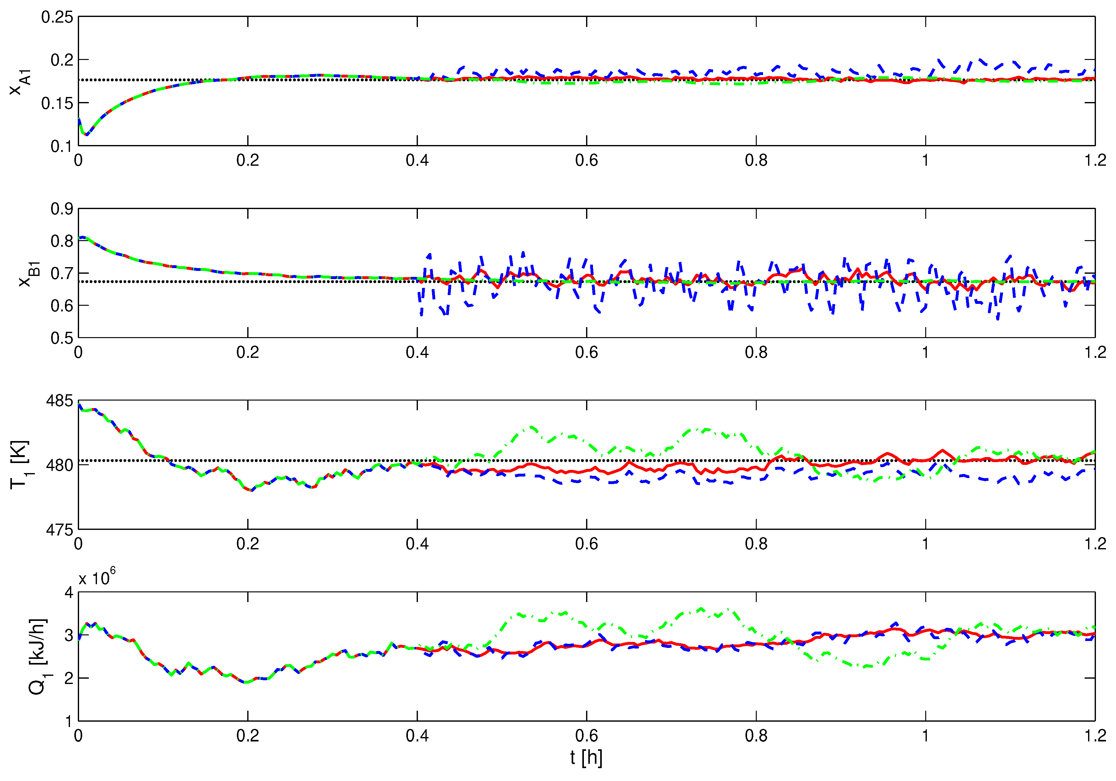
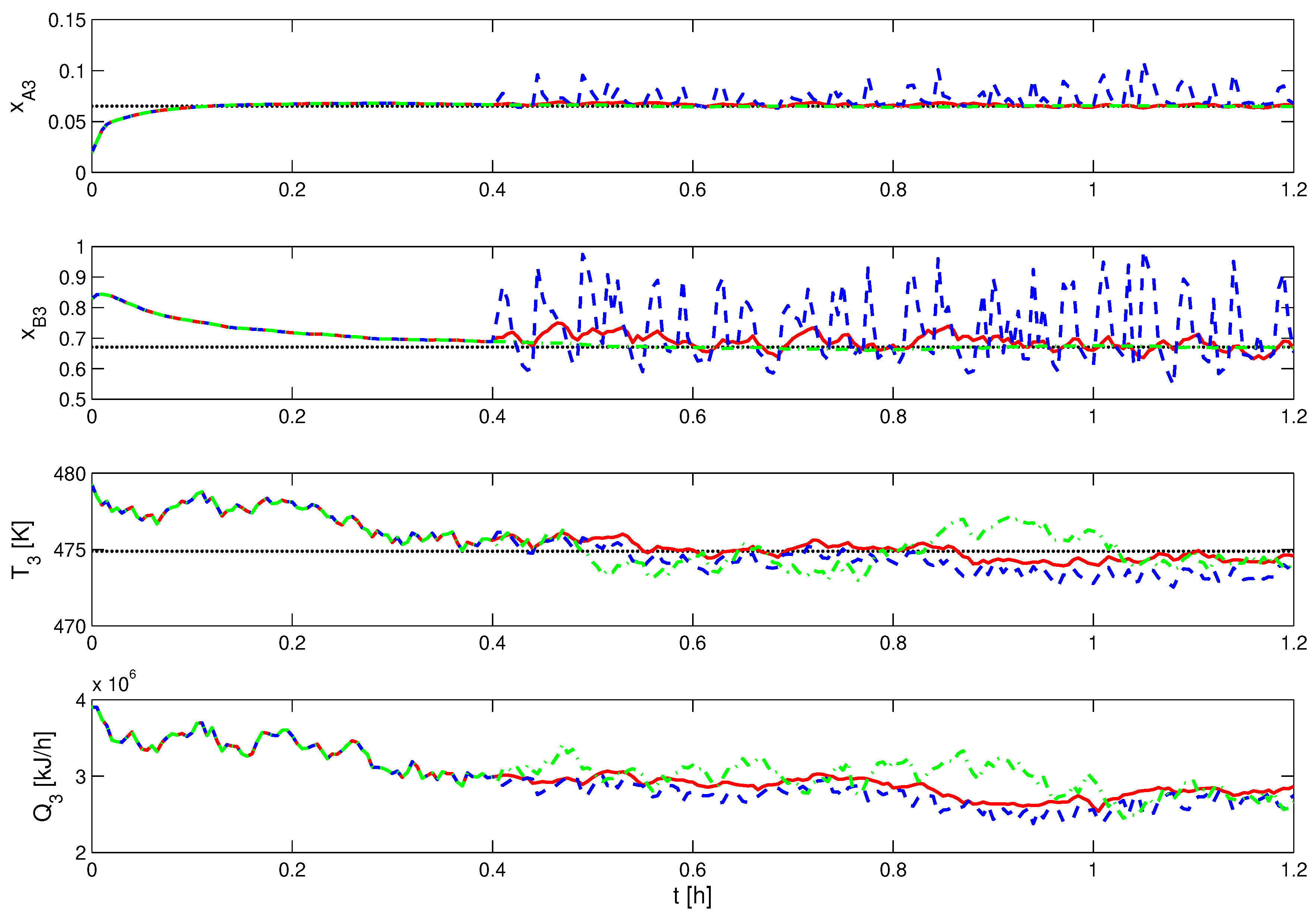
Figure 2, Figure 3 and Figure 4 show the trajectories of the subsystem states x A i , x B i and T i , and heat input Q i of subsystem 1 (the first CSTR), subsystem 2 (the second CSTR) and subsystem 3 (the separator) respectively generated by the three different schemes for a simulation duration of t f = 1.2   h . We can see from the three figures that all of the proposed distributed MHE-LMPC, scheme II and scheme III can drive the process state to the desired steady-state. At the initial time, the observers in each subsystems are applied for 80 sampling intervals to drive the state estimates to a small neighborhood of the actual state values. Starting from t b = 80 , the MHE is activated in the proposed scheme. It can be seen that the state trajectories of the three subsystems can all track the steady-state values well. However in scheme II, the trajectories of temperature T i , i = 1 , 2 , 3 , exhibit relatively large oscillations around the steady-state. The figures also show that the proposed distributed MHE-LMPC gives overall the best control performance. This is because in the state estimation part of the three different control strategies, the proposed scheme takes advantages of both the stability property of the nonlinear observer and the optimality of the MHE.
In order to further illustrate the role of different state estimation methods played in the control strategies, the error of state estimations given by the proposed scheme, scheme II and scheme III are compared. Figure 5 illustrates the trajectories of the Euclidean norm of estimation errors of the three different schemes. Note that, in order to solve the problem of different estimation error magnitudes of different states, the error of each state is normalized based on the maximum estimation error of all the three different schemes. Figure 5 shows that all of the three estimation methods adopted by the three control strategies can track the trends of the system real states. We can also see from the figure that the estimation error of the proposed scheme is the smallest among the three schemes. The maximum estimation errors calculated by the state estimation in the proposed scheme, scheme II and scheme III are 1.2575, 1.2627 and 1.7516, respectively. The average estimation error in the simulation time are also calculated. They are 0.4738, 0.5494 and 0.8320 corresponding to the three different state estimation methods. Theses results show that the proposed scheme gives the best estimation performance in the three different schemes.
In the simulations, the overall control performance of the different control designs for the entire system is also compared by a performance index as follows:
J = t k = t 1 t f x ( t k ) T Q c x ( t k ) + u ( t k ) T R c u ( t k ) ,
where t f = 1.2 h denotes the simulation time, x ( k ) denotes system state at time instant t k , Q c and R c are based on the weighting matrices Q c , i and R c , i in local LMPC, such that Q c = d i a g ( [ Q c , 1 Q c , 2 Q c , 3 ] ) and R c = d i a g ( [ R c , 1 R c , 2 R c , 3 ] ) . The entire system performance calculated by index Equation (19) of the proposed distributed MHE-LMPC, scheme II and scheme III are 6189.1, 6619.9 and 9499.2 respectively. The result further confirms that the proposed strategy gives the best control performance.
Another set of simulations has also been carried out to compare the overall performance of these three distributed control schemes. For different simulation run in the set of simulations, different initial states, initial guesses, process disturbances and output measurement noises are adopted. The results of 15 simulation runs are shown in Table 2. From simulation run 1 to run 10, the estimation horizon of local MHE in the proposed distributed MHE-LMPC and local MHE in scheme III is N e = 5 . From the simulation results, we can see that the proposed distributed MHE-LMPC gives the best overall performance and scheme III gives the worst performance. From simulation run 11 to run 15, the effects of horizon N e on the performance of different schemes are studied. All the parameters of these three control strategies are the same except N e . The results shown that with the increase of N e , the performance of scheme III improves dramatically, it is better than scheme II when N e is larger than 10. However the proposed MHE-LMPC is less sensitive to the value of moving horizon, and can obtain satisfactory result even when N e is small.
In Table 3, the mean evaluation times of the local MHE in the proposed scheme, the observer in scheme II and local MHE in scheme III are compared when N e = 5 and N e = 15 . Matlab in a computer with Intel Core i5, 4GB RAM is used for the evaluations. From Table 3, we can see that compared with the local MHE in scheme III, although the local MHE in the proposed scheme uses the nonlinear observer to calculate the reference state estimate, the evaluation time of this part is negligible. However, from small N e to large N e , the computation time both of the proposed scheme and scheme III increase significantly.

6. Conclusions and Future Work

Distributed schemes are very important for large-scale nonlinear systems. In this work, a distributed Lyapunov model predictive control based on distributed state estimation is proposed for these complex processes consisting of multiple interacting subsystems. Subsystems can exchange information through a communication network. During a short period from the initial time, the state estimates of each subsystem can reach a small neighborhood of the actual state values by a nonlinear observer due to its fast convergence. Meanwhile, the subsystem observer provides state estimates to subsystem Lyapunov MPC during this short period. After that, each subsystem state estimate sapproach switches to observer-enhanced moving horizon estimation, the MHE is evaluated to provide optimal estimates of subsystem state to the Lyapunov-based MPC. The detailed implementation algorithm of the proposed distributed strategy is given in the paper. Finally, the proposed scheme is used in a chemical process with two continuous stirred tank reactors and a flash tank separator to verify its applicability. The subsystem observer, the observer-enhanced MHE and Lyapunov MPC of this chemical process are designed. The performance of the proposed schemes are compared with two different distributed control strategies from different aspects to illustrate its effectiveness.
As for future work, the proposed scheme may be extended to handle communication delays and data losses. The performance and applicability of the proposed distributed scheme may also be further investigated by applying to large-scale industrial-relevant processes.

Author Contributions

Conceptualization, J.Z. and J.L.; methodology, J.Z. and J.L.; software, J.Z.; data curation, J.Z.; writing—original draft preparation, J.Z.; writing—review and editing, J.L.; funding acquisition, J.Z. All authors have read and agreed to the published version of the manuscript.

Funding

This work is supported by National Natural Science Foundation of China under Grant 61503257, 61773366; and the University of Alberta is acknowledged.

Data Availability Statement

Not applicable.

Conflicts of Interest

The authors declare no conflict of interest.

References

  1. Scattolini, R. Architectures for distributed and hierarchical model predictive control—A review. J. Process Control 2009, 19, 723–731. [Google Scholar] [CrossRef]
  2. Christofides, P.D.; Scattolini, R.; de la Peña, D.M.; Liu, J. Distributed model predictive control: A tutorial review and future research directions. Comput. Chem. Eng. 2013, 51, 21–41. [Google Scholar] [CrossRef]
  3. Rocha, R.R.; Oliveira-Lopes, L.C.; Christofides, P.D. Partitioning for distributed model predictive control of nonlinear processes. Chem. Eng. Res. Des. 2018, 139, 116–135. [Google Scholar] [CrossRef]
  4. Zhang, A.; Yin, X.; Liu, J. Distributed economic model predictive control of wastewater treatment plants. Chem. Eng. Res. Des. 2019, 141, 144–155. [Google Scholar] [CrossRef]
  5. Hassanzadeh, B.; Liu, J.; Forbes, J.F. A bi-level optimization approach to coordination of distributed model predictive control systems. Ind. Eng. Chem. Res. 2017, 57, 1516–1530. [Google Scholar] [CrossRef]
  6. Hassanzadeh, B.; Hallas, P.; Liu, J.; Forbes, J.F. Distributed model predictive control of nonlinear systems based on price-driven coordination. Ind. Eng. Chem. Res. 2016, 55, 9711–9724. [Google Scholar] [CrossRef]
  7. Rashedi, M.; Liu, J.; Huang, B. Triggered communication in distributed adaptive high-gain EKF. IEEE Trans. Ind. Inform. 2018, 14, 58–68. [Google Scholar] [CrossRef]
  8. Zeng, J.; Liu, J.; Zou, T.; Yuan, D. Distributed extended Kalman filtering for wastewater treatment processes. Ind. Eng. Chem. Res. 2016, 55, 7720–7729. [Google Scholar] [CrossRef]
  9. Wilson, D.; Agarwal, M.; Rippin, D. Experiences implementing the extended Kalman filter on an industrial batch reactor. Comput. Chem. Eng. 1998, 22, 1653–1672. [Google Scholar] [CrossRef]
  10. Farina, M.; Ferrari-Trecate, G.; Scattolini, R. Distributed moving horizon estimation for linear constrained systems. IEEE Trans. Autom. Control 2010, 55, 2462–2475. [Google Scholar] [CrossRef] [Green Version]
  11. Farina, M.; Ferrari-Trecate, G.; Scattolini, R. Distributed moving horizon estimation for nonlinear constrained systems. Int. J. Robust Nonlinear Control 2012, 22, 123–143. [Google Scholar] [CrossRef] [Green Version]
  12. Zhang, J.; Liu, J. Distributed moving horizon estimation for nonlinear systems with bounded uncertainties. J. Process Control 2013, 23, 1281–1295. [Google Scholar] [CrossRef]
  13. Liu, J. Moving horizon state estimation for nonlinear systems with bounded uncertainties. Chem. Eng. Sci. 2013, 93, 376–386. [Google Scholar] [CrossRef]
  14. Yin, X.; Arulmaran, K.; Liu, J.; Zeng, J. Subsystem decomposition and configuration for distributed state estimation. AIChE J. 2016, 62, 1995–2003. [Google Scholar] [CrossRef]
  15. Yin, X.; Liu, J. Distributed moving horizon state estimation of two-time-scale nonlinear systems. Automatica 2017, 79, 152–161. [Google Scholar] [CrossRef]
  16. Yin, X.; Decardi-Nelson, B.; Liu, J. Subsystem decomposition and distributed moving horizon estimation of wastewater treatment plants. Chem. Eng. Res. Des. 2018, 134, 405–419. [Google Scholar] [CrossRef]
  17. Yin, X.; Zeng, J.; Liu, J. Forming distributed state estimation network from decentralized estimators. IEEE Trans. Control Syst. Technol. 2019, 27, 2430–2443. [Google Scholar] [CrossRef]
  18. Yin, X.; Liu, J. Subsystem decomposition of process networks for simultaneous distributed state estimation and control. AIChE J. 2019, 65, 904–914. [Google Scholar] [CrossRef]
  19. Zhang, J.; Liu, J. Lyapunov-Based MPC with Robust Moving Horizon Estimation and its Triggered Implementation. AIChE J. 2013, 59, 4273–4286. [Google Scholar] [CrossRef]
  20. Ellis, M.; Zhang, J.; Liu, J.; Christofides, P. Robust moving horizon estimation based output feedback economic model predictive control. Syst. Control Lett. 2014, 68, 101–109. [Google Scholar] [CrossRef]
  21. Christofides, P.D.; Davis, J.F.; El-Farra, N.H.; Clark, D.; Harris, K.R.D.; Gipson, J.N. Smart plant operations: Vision, progress and challenges. AIChE J. 2007, 53, 2734–2741. [Google Scholar] [CrossRef]
  22. Qi, W.; Liu, J.; Christofides, P.D. A distributed control framework for smart grid development: Energy/water system optimal operation and electric grid integration. J. Process Control 2011, 21, 1504–1516. [Google Scholar] [CrossRef]
  23. Ahrens, J.H.; Khalil, H.K. High-gain observers in the presence of measurement noise: A switched-gain approach. Automatica 2009, 45, 936–943. [Google Scholar] [CrossRef]
  24. Liu, S.; Liu, J. Distributed Lyapunov-based model predictive control with neighbor-to-neighbor communication. AIChE J. 2014, 60, 4124–4133. [Google Scholar] [CrossRef]
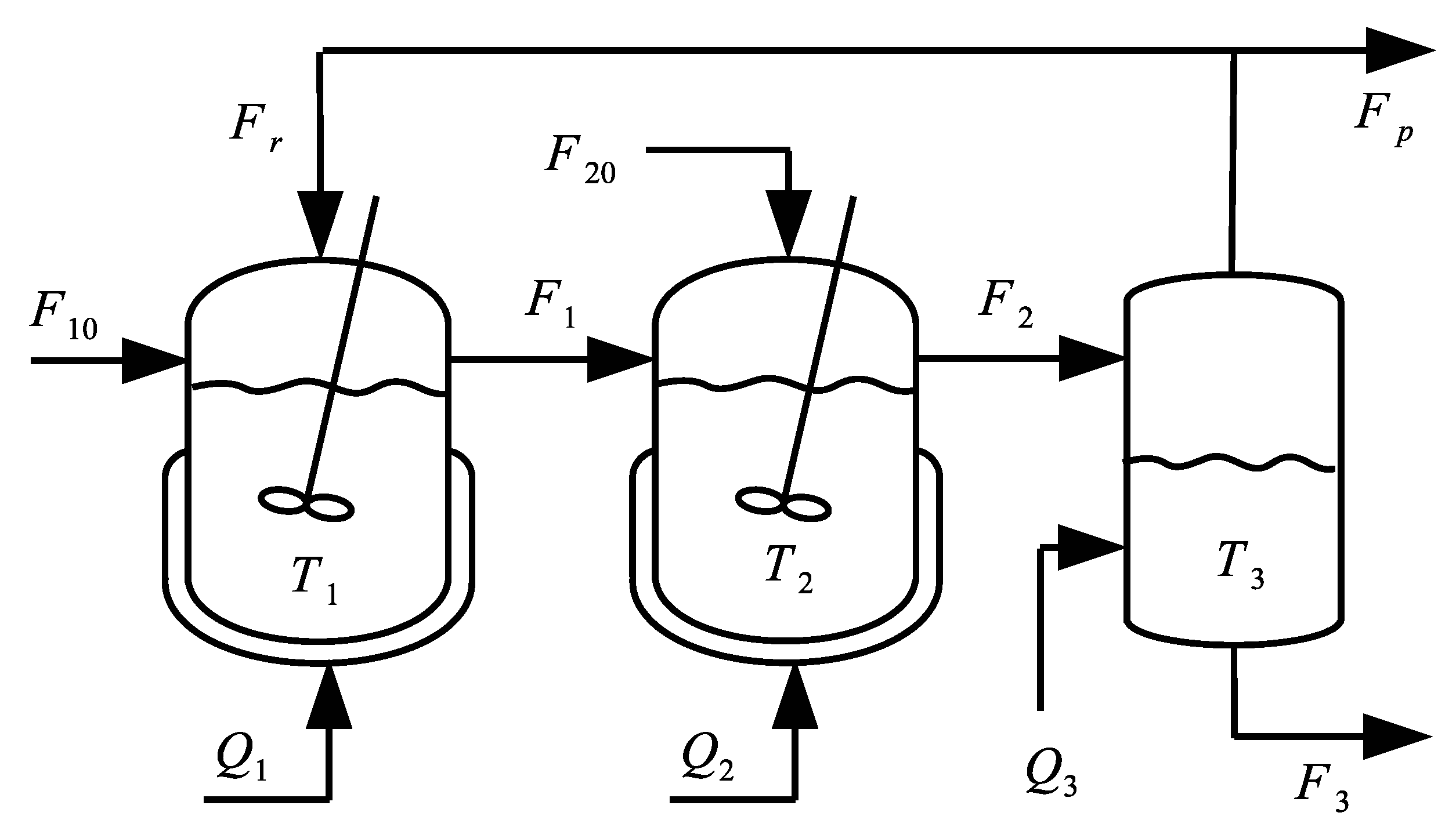
Figure 1. Reactor-separator process with a recycle stream.
Mathematics 09 01327 g001
Figure 2. States and input trajectories of subsystem 1 given by the proposed distributed MHE-LMPC (solid line), scheme II (dash-dotted line) and scheme III (dashed line). The set points of states are denoted as dotted line.
Mathematics 09 01327 g002
Figure 3. States and input trajectories of subsystem 2 given by the proposed distributed MHE-LMPC (solid line), scheme II (dash-dotted line) and scheme III (dashed line). The set points of states are denoted as dotted line.
Mathematics 09 01327 g003
Figure 4. States and input trajectories of subsystem 3 given by the proposed distributed MHE-LMPC (solid line), scheme II (dash-dotted line) and scheme III (dashed line). The set points of states are denoted as dotted line.
Mathematics 09 01327 g004
Figure 5. Trajectories of the Euclidean norm estimation errors calculated by the proposed scheme (solid lines) and the scheme II (dash-dotted line) and the scheme III (dashed line).
Mathematics 09 01327 g005
Table 1. Steady state values.
VariableSteady State ValueVariableSteady State Value
x A 1 s 0.1763 T 1 s 480.3165  [K]
x A 2 s 0.1965 T 2 s 472.7863  [K]
x A 3 s 0.0651 T 3 s 474.8877  [K]
x B 1 s 0.6731 Q 1 s 2.9 × 10 6  [KJ/h]
x B 2 s 0.6536 Q 2 s 1.0 × 10 6  [KJ/h]
x B 3 s 0.6703 Q 3 s 2.9 × 10 6  [KJ/h]
Table 2. Control performance comparison of the closed-loop process with various initial conditions, initial estimation guess, process disturbances and output measurement noise under three different schemes: (I) the proposed distributed MHE-LMPC; (II) the distributed LMPC based on the deterministic nonlinear observer (7); (III) a distributed MHE-LMPC scheme implemented following the proposed scheme but without constraint (9e)–(9h) in the local MHE design.
RunScheme IScheme IIScheme III
16522.4 ( N e = 5 )7470.68244.6 ( N e = 5 )
29338.0 ( N e = 5 )9972.115,760.0 ( N e = 5 )
34898.0 ( N e = 5 )5084.96442.7 ( N e = 5 )
44913.3 ( N e = 5 )5087.15711.2 ( N e = 5 )
56476.6 ( N e = 5 )6971.08710.7 ( N e = 5 )
65874.9 ( N e = 5 )6355.38789.3 ( N e = 5 )
77102.8 ( N e = 5 )8158.99872.5 ( N e = 5 )
84005.1 ( N e = 5 )4325.25986.3 ( N e = 5 )
95120.1 ( N e = 5 )5483.06011.1 ( N e = 5 )
106813.5 ( N e = 5 )7592.611,156.2 ( N e = 5 )
116263.8 ( N e = 5 )6717.09571.7 ( N e = 5 )
126169.7 ( N e = 8 )6717.07052.0 ( N e = 8 )
136126.9 ( N e = 10 )6717.06455.5 ( N e = 10 )
146101.1 ( N e = 12 )6717.06209.4 ( N e = 12 )
156073.4 ( N e = 15 )6717.06079.9 ( N e = 15 )
Table 3. Comparison of mean evaluation time of different schemes for each subsystem.
HorizonSub-SystemScheme II (s)Scheme II (s)Scheme III (s)
N e = 5 # 1 2.32800.00231.6878
# 2 1.71620.00221.6660
# 3 2.26000.00221.6625
N e = 15 # 1 29.94270.002526.7433
# 2 25.32350.002722.6616
# 3 28.71940.002726.0822
Publisher’s Note: MDPI stays neutral with regard to jurisdictional claims in published maps and institutional affiliations.