Analysis of a New Nonlinear Interpolatory Subdivision Scheme on σ Quasi-Uniform Grids

Abstract

In this paper, we introduce and analyze the behavior of a nonlinear subdivision operator called PPH, which comes from its associated PPH nonlinear reconstruction operator on nonuniform grids. The acronym PPH stands for Piecewise Polynomial Harmonic, since the reconstruction is built by using piecewise polynomials defined by means of an adaption based on the use of the weighted Harmonic mean. The novelty of this work lies in the generalization of the already existing PPH subdivision scheme to the nonuniform case. We define the corresponding subdivision scheme and study some important issues related to subdivision schemes such as convergence, smoothness of the limit function, and preservation of convexity. In order to obtain general results, we consider σ quasi-uniform grids. We also perform some numerical experiments to reinforce the theoretical results.

1. Introduction

Subdivision schemes are closely related to reconstruction operators. They have been used in the last few decades in many applications ranging from the numerical solution of partial differential equations to image processing and computer-aided geometric design. Subdivision schemes give simple and fast algorithms to approximate the limit function from a set of initial data at a coarse resolution level. There is an method of immediately generating subdivision schemes from reconstruction operators and more specifically from prediction operators [1,2,3]. Due to this connection, subdivision schemes inherit many of the properties of their associated reconstruction operators. In particular, the subdivision scheme is nonlinear if the reconstruction operator is nonlinear and it is said interpolatory if it comes from a reconstruction operator that is an interpolation.

Nonlinear subdivision schemes have emerged as good candidates to adapt to the concrete data in use. The research in this field has expanded, with new contributions each year, and has received the attention of many researchers; see for example [4,5,6,7,8]. Nonlinearity means data-dependent subdivision schemes, which may also involve nonlinear operations in their definition. Then, by definition, they are designed to overcome certain drawbacks that appear when dealing with their linear counterparts, such as bad behavior in the presence of isolated discontinuities for instance. An example of these types of operators was defined in [1] and was named PPH (Piecewise Polynomial Harmonic). This scheme basically consists on a clever modification of the classical four-point Lagrange subdivision scheme. Several studies have been carried out about their properties and performance in different applications, see for example [1,9,10]. Two main purposes of this subdivision scheme are related to dealing with data containing isolated discontinuities, reducing the undesirable effects, and preserving the convexity of the initial data while maintaining a centered support based on four points.

In [11], the authors extended the definition of the PPH reconstruction operator to nonuniform grids. In turn, this fact allows us to extend the PPH subdivision scheme to nonuniform grids and to carry out a parallel study in this new scenario. In order to overcome some technical difficulties in the theoretical proofs, we restricted some results to $\sigma$ quasi-uniform grids. The resultant scheme is quite interesting in terms of applications due to the almost $C^1$ smoothness of the limit function, allowing us to approximate accurately continuous functions with corners, and due to appropriate properties regarding convexity preservation of the initial data; see [9]. In this paper, we focus on proving the convergence of the scheme towards an almost $C^1$ limit function and we address numerically the issue of stability, which is a central issue in order to be useful for applications.

The paper is organized as follows: Section 2 is devoted to a review of the PPH reconstruction operator over nonuniform grids. Section 3 presents a short review about Harten’s interpolatory multiresolution setting, which is closely connected to interpolatory subdivision schemes. In Section 4, we define the associated subdivision scheme, which we show amounts to the PPH subdivision scheme when use a restriction to uniform grids. The definition is given for general nonuniform meshes, although in order to establish some theoretical results, we consider $\sigma$ quasi-uniform meshes. In Section 5, we analyze the main issues about subdivision schemes. In particular, we prove some results about convergence, smoothness of the limit function, and convexity preservation. In Section 6, we carry out some numerical tests to check the theoretical smoothness of the limit function and the performance of the nonlinear subdivision scheme. Finally, we give some conclusions in Section 7.

2. A Nonlinear PPH Reconstruction Operator on Nonuniform Grids

In this section, we review the definition of the nonlinear reconstruction that gives rise to the nonlinear subdivision scheme under study in this article. More information about this reconstruction operator can be found in [1,11,12].

Let us define a nonuniform grid $X={\left(x_i\right)}_{i\in \mathbb{Z}}.$ Let us also denote $h_i:=x_i-x_{i-1},$ the nonuniform spacing between abscissae. Let us consider the set of values $\{f_{j-1},f_j,f_{j+1},f_{j+2}\}$ for some $j\in \mathbb{Z}$ corresponding to the abscissae $\{x_{j-1},x_j,x_{j+1},x_{j+2}\}$ of the nonuniform grid $X.$

We need to introduce the definition of the second-order divided differences

$$\begin{array}{cc}\hfill D_j& :=f[x_{j-1},x_j,x_{j+1}]=\frac{f_{j-1}}{h_j(h_j+h_{j+1})}-\frac{f_j}{h_j{h}_{j+1}}+\frac{f_{j+1}}{h_{j+1}(h_j+h_{j+1})},\hfill \\ \hfill D_{j+1}& :=f[x_j,x_{j+1},x_{j+2}]=\frac{f_j}{h_{j+1}(h_{j+1}+h_{j+2})}-\frac{f_{j+1}}{h_{j+1}{h}_{j+2}}+\frac{f_{j+2}}{h_{j+2}(h_{j+1}+h_{j+2})},\hfill \end{array}$$

(1)

and the weighted arithmetic mean of $D_j$ and $D_{j+1}$ defined as

$$M_j=w_{j,0}{D}_j+w_{j,1}{D}_{j+1},$$

(2)

with the weights

$$\begin{array}{cc}\hfill w_{j,0}& ={\displaystyle \frac{h_{j+1}+2h_{j+2}}{2(h_j+h_{j+1}+h_{j+2})}},\hfill \\ \hfill w_{j,1}& ={\displaystyle \frac{h_{j+1}+2h_j}{2(h_j+h_{j+1}+h_{j+2})}}=1-w_{j,0}.\hfill \end{array}$$

(3)

We require also some definitions and lemmas that appear in [11].

Definition 1.

Given $x,y\in \mathbb{R},$ and $w_x,w_y\in \mathbb{R}$ such that $w_x>0,$ $w_y>0,$ and $w_x+w_y=1,$ we denote $\tilde{V}$ as the function

$$\tilde{V}(x,y)=\left\{\begin{array}{cc}{\displaystyle \frac{xy}{w_{x}y+w_{y}x}}& \mathit{if}xy>0,\hfill \\ 0& \mathit{otherwise}.\hfill \end{array}\right.$$

(4)

Lemma 1.

If $x\ge 0$ and $y\ge 0,$ the harmonic mean is bounded as follows:

$$\tilde{V}(x,y)<min\left\{{\displaystyle \frac{1}{w_x}}x,{\displaystyle \frac{1}{w_y}}y\right\}\le {\displaystyle \frac{1}{w_x}}x.$$

(5)

Lemma 2.

Let $a>0$ be a fixed positive real number, and let $x\ge a$ and $y\ge a.$ If $|x-y|=O\left(h\right)$ and $xy>0,$ then the weighted harmonic mean is also close to the weighted arithmetic mean $M(x,y)=w_{x}x+w_{y}y,$

$$|M(x,y)-\tilde{V}(x,y)|={\displaystyle \frac{w_x{w}_y}{w_{x}y+w_{y}x}}{(x-y)}^2=O\left(h^2\right).$$

(6)

We review the following definition for the PPH reconstruction on nonuniform meshes. The details and main properties of this reconstruction operator can be found in [11,12].

Definition 2 (PPH reconstruction).

Let $X={\left(x_i\right)}_{i\in \mathbb{Z}}$ be a nonuniform mesh. Let $f={\left(f_i\right)}_{i\in \mathbb{Z}}$ be a sequence in $l_{\infty }\left(\mathbb{Z}\right).$ Let $D_j$ and $D_{j+1}$ be the second-order divided differences, and for each $j\in \mathbb{Z}$, let us consider the modified values $\{{\tilde{f}}_{j-1},{\tilde{f}}_j,{\tilde{f}}_{j+1},{\tilde{f}}_{j+2}\}$ built according to the following rule:

• Case 1: If $|D_j|\le |D_{j+1}|$

  $$\left\{\begin{array}{cc}{\tilde{f}}_i=\hfill & f_i,j-1\le i\le j+1,\hfill \\ {\tilde{f}}_{j+2}=\hfill & \frac{-1}{{\gamma }_{j,2}}({\gamma }_{j,-1}{f}_{j-1}+{\gamma }_{j,0}{f}_j+{\gamma }_{j,1}{f}_{j+1})+\frac{{\tilde{V}}_j}{{\gamma }_{j,2}},\hfill \end{array}\right.$$

  (7)
• Case 2: If $|D_j|>|D_{j+1}|$

  $$\left\{\begin{array}{cc}{\tilde{f}}_{j-1}=\hfill & \frac{-1}{{\gamma }_{j,-1}}({\gamma }_{j,0}{f}_j+{\gamma }_{j,1}{f}_{j+1}+{\gamma }_{j,2}{f}_{j+2})+\frac{{\tilde{V}}_j}{{\gamma }_{j,-1}},\hfill \\ {\tilde{f}}_i=\hfill & f_i,j\le i\le j+2,\hfill \end{array}\right.$$

  (8)

where ${\gamma }_{j,i},i=-1,0,1,2$ are given by

$$\begin{array}{c}{\gamma }_{j,-1}={\displaystyle \frac{h_{j+1}+2h_{j+2}}{2h_j(h_{j+1}+h_j)(h_j+h_{j+1}+h_{j+2})}},\hfill \\ {\gamma }_{j,0}={\displaystyle \frac{1}{2h_{j+1}(h_j+h_{j+1}+h_{j+2})}}\left({\displaystyle \frac{h_{j+1}+2h_j}{h_{j+1}+h_{j+2}}}-{\displaystyle \frac{h_{j+1}+2h_{j+2}}{h_j}}\right),\hfill \\ {\gamma }_{j,1}={\displaystyle \frac{1}{2h_{j+1}(h_j+h_{j+1}+h_{j+2})}}\left({\displaystyle \frac{h_{j+1}+2h_{j+2}}{h_{j+1}+h_j}}-{\displaystyle \frac{h_{j+1}+2h_j}{h_{j+2}}}\right),\hfill \\ {\gamma }_{j,2}={\displaystyle \frac{h_{j+1}+2h_j}{2h_{j+2}(h_{j+1}+h_{j+2})(h_j+h_{j+1}+h_{j+2})}},\hfill \end{array}$$

(9)

and ${\tilde{V}}_j=\tilde{V}(D_j,D_{j+1}),$ with $\tilde{V}$ being the weighted harmonic mean defined in (4) with the weights $w_{j,0}$ and $w_{j,1}$ in (3). We define $\mathcal{R}\left(x\right)$ as the PPH nonlinear reconstruction operator given by

$$\mathcal{R}\left(x\right)={\mathcal{R}}_j\left(x\right),x\in [x_j,x_{j+1}],$$

(10)

where ${\mathcal{R}}_j\left(x\right)$ is the unique interpolation polynomial that satisfies

$${\mathcal{R}}_j\left(x_i\right)={\tilde{f}}_i,j-1\le i\le j+2.$$

(11)

We can write the PPH reconstruction by using the middle point $x_{j+\frac{1}{2}}=\frac{x_j+x_{j+1}}{2}$ as

$${\mathcal{R}}_j\left(x\right)={\tilde{a}}_{j,0}+{\tilde{a}}_{j,1}\left(x-x_{j+\frac{1}{2}}\right)+{\tilde{a}}_{j,2}{\left(x-x_{j+\frac{1}{2}}\right)}^2+{\tilde{a}}_{j,3}{\left(x-x_{j+\frac{1}{2}}\right)}^3,$$

(12)

where the the coefficients ${\tilde{a}}_{j,i},i=0,\dots ,3$ are calculated by imposing conditions (11). Depending on the local case, Case 1 or Case 2, the coefficients have different expressions.

Case 1. $|D_j|\le |D_{j+1}|$, In this case, the coefficients of the polynomial (12) take the form

$$\begin{array}{c}{\tilde{a}}_{j,0}={\displaystyle \frac{f_j+f_{j+1}}{2}}-{\displaystyle \frac{h_{j+1}^2}{4}}{\tilde{V}}_j,\hfill \\ {\tilde{a}}_{j,1}={\displaystyle \frac{-f_j+f_{j+1}}{h_{j+1}}}+{\displaystyle \frac{h_{j+1}^2}{4h_j+2h_{j+1}}}(D_j-{\tilde{V}}_j),\hfill \\ {\tilde{a}}_{j,2}={\tilde{V}}_j,\hfill \\ {\tilde{a}}_{j,3}=-{\displaystyle \frac{2}{2h_j+h_{j+1}}}(D_j-{\tilde{V}}_j).\hfill \end{array}$$

(13)

Case 2. $|D_j|>|D_{j+1}|$, In this case, we obtain the following coefficients for the polynomial (12)

$$\begin{array}{c}{\tilde{a}}_{j,0}={\displaystyle \frac{f_j+f_{j+1}}{2}}-{\displaystyle \frac{h_{j+1}^2}{4}}{\tilde{V}}_j,\hfill \\ {\tilde{a}}_{j,1}={\displaystyle \frac{-f_j+f_{j+1}}{h_{j+1}}}+{\displaystyle \frac{h_{j+1}^2}{2h_{j+1}+4h_{j+2}}}(-D_{j+1}+{\tilde{V}}_j),\hfill \\ {\tilde{a}}_{j,2}={\tilde{V}}_j,\hfill \\ {\tilde{a}}_{j,3}=-{\displaystyle \frac{2}{h_{j+1}+2h_{j+2}}}(-D_{j+1}+{\tilde{V}}_j).\hfill \end{array}$$

(14)

With the previous definitions and lemmas, we are now ready to introduce the PPH subdivision scheme. However, before doing this, we also review some basic concepts of Harten’s interpolatory multiresolution setting and its connection with subdivision schemes.

3. Harten’s Interpolatory Multiresolution Setting

Let us consider a set of nested grids in $\mathbb{R},$

$$X^k={\left\{x_i^k\right\}}_{i\in \mathbb{Z}},$$

and the point-value discretization

$$\begin{array}{cccc}\hfill {\mathcal{D}}_k:C_B& \left(\mathbb{R}\right)\hfill & & \to V^k\hfill \\ & f\hfill & & \mapsto f^k={\left(f_i^k\right)}_{i\in \mathbb{Z}}={\left(f\left(x_i^k\right)\right)}_{i\in \mathbb{Z}},\hfill \end{array}$$

(15)

where $V^k$ is the space of real sequences related to the resolution of $X^k$ and $C_B\left(\mathbb{R}\right)$ is the set of bounded continuous functions on $\mathbb{R}$.

A reconstruction operator ${\mathcal{R}}_k$ associated with this discretization is any right inverse of ${\mathcal{D}}_k$, which means that for all $f^k\in V^k,{\mathcal{R}}_k{f}^k\in C_B\left(\mathbb{R}\right),$ and ${\mathcal{D}}_k{\mathcal{R}}_k=I,$ that is

$$\begin{array}{cccc}\hfill {\mathcal{R}}_k:& V^k\hfill & & \to C_B\left(\mathbb{R}\right)\hfill \\ & f^k\hfill & & \mapsto {\mathcal{R}}_k{f}^k,\hfill \end{array}$$

(16)

$$\left({\mathcal{R}}_k{f}^k\right)\left(x_i^k\right)={\left(f_i^k\right)}_{i\in \mathbb{Z}}={\left(f\left(x_i^k\right)\right)}_{i\in \mathbb{Z}}.$$

The sequences ${\left\{{\mathcal{D}}_k\right\}}_{k\in \mathbb{N}}$ and ${\left\{{\mathcal{R}}_k\right\}}_{k\in \mathbb{N}}$ define a multiresolution transform [2]. The prediction operator, i.e., ${\mathcal{D}}_{k+1}{\mathcal{R}}_k:V^k\to V^{k+1}$, defines a subdivision scheme. Relation (16) implies that the subdivision scheme is interpolatory. If ${\mathcal{R}}_k$ is a nonlinear reconstruction operator, then the corresponding subdivision scheme $\mathcal{S}:={\mathcal{D}}_{k+1}{\mathcal{R}}_k$ becomes also nonlinear.

4. A Nonlinear PPH Subdivision Scheme on Nonuniform Grids

Let us consider a particular set of nonuniform nested grids $X^k={\left(x_i^k\right)}_{i\in \mathbb{Z}},$ $k\ge 0,$ generated from an initial grid $X^0.$

Definition 3.

Given $X^0={\left\{x_i\right\}}_{i\in \mathbb{Z}}$ as a nonuniform grid in $\mathbb{R},$ we define, for $k\in \mathbb{N}$ (the larger the k, the larger the resolution), as the set of nested grids given by $X^k={\left\{x_i^k\right\}}_{i\in \mathbb{Z}},$ where $x_{2i}^k=x_i^{k-1}$ and $x_{2i+1}^k=\frac{x_i^{k-1}+x_{i+1}^{k-1}}{2}.$

Let us also consider $h_i^k=x_i^k-x_{i-1}^k,$ the nonuniform spacing between abscissae. Given a set of control points $f^k={\left(f_i^k\right)}_{i\in \mathbb{Z}},$ we define the nonlinear PPH subdivision scheme as

$$\begin{array}{c}{f}_{2i}^{k+1}={\left(\mathcal{S}{f}^k\right)}_{2i}=f_i^k,\hfill \\ f_{2i+1}^{k+1}={\left(\mathcal{S}{f}^k\right)}_{2i+1}={\displaystyle \frac{f_i^k+f_{i+1}^k}{2}}-{\displaystyle \frac{{\left(h_{i+1}^k\right)}^2}{4}}{\tilde{V}}_i^k,\hfill \end{array}$$

(17)

where ${\tilde{V}}_i^k={\tilde{V}}_i^k(D_i^k,D_{i+1}^k)$ is given in (4) and it is computed with the weights ${\left(w_{i,0}^k\right)}_{i\in \mathbb{Z}},$ ${\left(w_{i,1}^k\right)}_{i\in \mathbb{Z}}$ is given in (3), and the second-order divided differences $D_i^k$ and $D_{i+1}^k$ are defined in (1).

Notice that the expression of the subdivision scheme at odd indexes coincides with the coefficient ${\tilde{a}}_0$ of the PPH reconstruction operator in (13) or (14) due to the fact that the defined subdivision scheme satisfies $\mathcal{S}={\mathcal{D}}_{k+1}{\mathcal{R}}_k.$ This means that the expression of the subdivision scheme is symmetric, even if the modification of the data has been carried out to the left (14) or to the right (13) for the concrete piece of the underlying reconstruction operator.

Suppose that the initial data come from a convex smooth function; then by definition through its associated reconstruction operator, we get a fourth-order accurate subdivision scheme. When the data come from an underlying smooth function with inflexion points, the order is reduced around these inflexion points [12]. The use of the weighted harmonic mean in Definition 17 guarantees certain adaptation near jump discontinuities. In the presence of an isolated singularity, we have two adjacent intervals where $D_i=O\left(1\right)$ and $D_{i+1}=O(1/{\left(h^k\right)}^2),$ or $D_i=O(1/{\left(h^k\right)}^2)$ and $D_{i+1}=O\left(1\right),$ with $h^k:=\underset{j\in \mathbb{Z}}{max}{h}_j^k.$ For these cases, the harmonic mean maintains an order of ${\tilde{V}}_i=O\left(1\right).$ If both $D_i$ and $D_{i+1}$ are affected by discontinuity, then no adaption takes place. However, this situation occurs only in the prediction of one value per scale and per discontinuity.

It is also interesting to remark that, for uniform meshes, i.e., $h_i=h\forall i,$ then all of the given expressions reduce to equivalent expressions in [1] valid only for the uniform case.

Notice that Definition 17 of the PPH subdivision schemes was introduced for general nonuniform meshes. From now on, one needs to take into account that some results are true for general grids while others require restriction to a particular type of nonlinear mesh that is the most common in practice.

In next the section, we study some main issues about the defined subdivision scheme. In particular we prove convergence, almost $C^1$ smoothness in the limit function, and we provide a result concerning convexity preservation.

5. Main Properties of the PPH Subdivision Scheme in Nonuniform Meshes

We start the section with some definitions taken from [1] that are used in the rest of the article.

Definition 4.

A nonlinear subdivision scheme is called uniformly convergent if for every set of initial data $f^0\in l_{\infty }\left(\mathbb{Z}\right)$, there exists a continuous function ${\mathcal{S}}^{\infty }{f}^0\in C\left(\mathbb{R}\right)$, such that

$$\underset{k\to \infty }{lim}||\mathcal{S}{f}^k-{\mathcal{S}}^{\infty }{f}^0(2^{-k}·){||}_{l_{\infty }\left(\mathbb{Z}\right)}=0.$$

Definition 5.

A convergent nonlinear subdivision scheme is called stable if there exists a constant C such that for every pair of initial data $f^0,{\tilde{f}}^0\in l_{\infty }\left(\mathbb{Z}\right)$,

$$||{\mathcal{S}}^{\infty }{f}^0-{\mathcal{S}}^{\infty }{\tilde{f}}^0{||}_{L^{\infty }}\le C||f^0-{\tilde{f}}^0{||}_{l_{\infty }\left(\mathbb{Z}\right)}.$$

Definition 6.

Let $N\ge 0$ be a fixed integer. A nonlinear interpolatory subdivision scheme has the property of polynomial reproduction of order N if for all $P\in {\Pi }_N,$ where ${\Pi }_N$ stands for the vector space of polynomials of degree less or equal to $N,$ we have $\mathcal{S}p=\tilde{p}$, where p and $\tilde{p}$ are defined by $p_k=P(2^{-k}·)$ and ${\tilde{p}}_k=P(2^{-(k+1)}·)$.

Definition 7.

A nonlinear subdivision scheme is called bounded if there exists a constant $C>0$ such that

$${||\mathcal{S}f||}_{l_{\infty }\left(\mathbb{Z}\right)}\le {C||f||}_{l_{\infty }\left(\mathbb{Z}\right)}\forall f\in l_{\infty }\left(\mathbb{Z}\right).$$

Definition 8.

A nonlinear subdivision scheme is called Lipschitz continuous if there exists a constant $C>0$ such that, for every $f,g\in l_{\infty }\left(\mathbb{Z}\right)$, the following is verified:

$$||\mathcal{S}f-{\mathcal{S}g||}_{l_{\infty }\left(\mathbb{Z}\right)}\le C||f-{g||}_{l_{\infty }\left(\mathbb{Z}\right)}.$$

(18)

We can now provide some basic results before addressing the convergence of the scheme. In order to prove the coming theoretical results, we work with $\sigma$ quasi-uniform grids, according to the following definition:

Definition 9.

A nonuniform mesh $X={\left(x_i\right)}_{i\in \mathbb{Z}}$ is said to be a σ quasi-uniform mesh if there exist $h_{min}=\underset{i\in \mathbb{Z}}{min}{h}_i,$ $h_{max}=\underset{i\in \mathbb{Z}}{max}{h}_i,$ and a finite constant σ such that $\frac{h_{max}}{h_{min}}\le \sigma .$

Proposition 1.

The nonlinear subdivision scheme associated wtih the PPH reconstruction:

(1) reproduces polynomials of degree $N\le 2,$

(2) is bounded, and

(3) is Lipschitz continuous.

Proof. 

(1) If f is a polynomial of degree less or equal to 2,

$$D_j=D_{j+1}={\tilde{V}}_j,$$

therefore, the proposed scheme reproduces polynomials of degree 2.

(2) By definition of the PPH subdivision scheme for a given $j\in \mathbb{Z}$, we have that

$${\left(\mathcal{S}f\right)}_{2j}=f_j,$$

$${\left(\mathcal{S}f\right)}_{2j+1}=\left\{\begin{array}{cc}\frac{f_j+f_{j+1}}{2}-\frac{{\left(h_{j+1}\right)}^2}{4}{\tilde{V}}_j\hfill & if{D}_j{D}_{j+1}>0,\hfill \\ \frac{f_j+f_{j+1}}{2}\hfill & otherwise.\hfill \end{array}\right.$$

Using $|D_j|\le \frac{{4||f||}_{l_{\infty }\left(\mathbb{Z}\right)}}{2h_{min}^2},$ $|D_{j+1}|\le \frac{{4||f||}_{l_{\infty }\left(\mathbb{Z}\right)}}{2h_{min}^2},$ we obtain

$$\begin{array}{c}\hfill |\frac{{\left(h_{j+1}\right)}^2}{4}{\tilde{V}}_j|\le \frac{{\left(h_{j+1}\right)}^2}{4}max\{|D_{j+1}|,|D_j|\}\le \frac{{\sigma }^2}{2}{||f||}_{l_{\infty }\left(\mathbb{Z}\right)}.\end{array}$$

Thus,

$${||\mathcal{S}f||}_{l_{\infty }\left(\mathbb{Z}\right)}\le (1+\frac{{\sigma }^2}{2}){||f||}_{l_{\infty }\left(\mathbb{Z}\right)},$$

and therefore the nonlinear subdivision scheme is bounded.

(3) Let us consider $\left\{f\right\},\left\{g\right\}\in l_{\infty }\left(\mathbb{Z}\right)$.

Clearly,

$${|\left(\mathcal{S}f\right)}_{2j}-{\left(\mathcal{S}g\right)}_{2j}|=|f_j-g_j{|\le ||f-g||}_{l_{\infty }\left(\mathbb{Z}\right)}.$$

Since

$$|\frac{f_j+f_{j+1}}{2}-\frac{g_j+g_{j+1}}{2}{|\le ||f-g||}_{l_{\infty }\left(\mathbb{Z}\right)},$$

to estimate the odd components ${|\left(\mathcal{S}f\right)}_{2j+1}-{\left(\mathcal{S}g\right)}_{2j+1}|$, we simply need to estimate the terms

$$\frac{{\left(h_{j+1}\right)}^2}{4}{\tilde{V}}_j\left(f\right),\frac{{\left(h_{j+1}\right)}^2}{4}{\tilde{V}}_j\left(g\right),$$

or

$$\frac{{\left(h_{j+1}\right)}^2}{4}{\tilde{V}}_j\left(f\right)-\frac{{\left(h_{j+1}\right)}^2}{4}{\tilde{V}}_j\left(g\right),$$

according to the sign of $D_j\left(f\right)D_{j+1}\left(f\right)$ and $D_j\left(g\right)D_{j+1}\left(g\right)$.

(a) Suppose $D_j\left(f\right)D_{j+1}\left(f\right)>0$ and $D_j\left(g\right)D_{j+1}\left(g\right)\le 0$. In particular, $D_{j+1}\left(f\right)D_{j+1}\left(g\right)\le 0$ or $D_j\left(f\right)D_j\left(g\right)\le 0$. In the first case, we write

$$\begin{array}{ccc}\hfill |\frac{{\left(h_{j+1}\right)}^2}{4}{\tilde{V}}_j\left(f\right)|& \le & \frac{{\left(h_{max}\right)}^2}{4}\frac{|D_{j+1}\left(f\right)|}{w_{1,j}}\hfill \\ & \le & \frac{{\left(h_{max}\right)}^2}{4}\frac{|D_{j+1}\left(f\right)-D_{j+1}\left(g\right)|}{w_{1,j}}\hfill \\ & \le & \frac{{\left(h_{max}\right)}^2}{4}\frac{4}{2{\left(h_{min}\right)}^2}2\sigma ||f-{g||}_{l_{\infty }\left(\mathbb{Z}\right)}\hfill \\ & \le & {\sigma }^3||f-{g||}_{l_{\infty }\left(\mathbb{Z}\right)},\hfill \end{array}$$

and in the second case, we similarly obtain

$$\begin{array}{ccc}\hfill |\frac{{\left(h_{j+1}\right)}^2}{4}{\tilde{V}}_j\left(f\right)|& \le & \frac{{\left(h_{max}\right)}^2}{4}\frac{|D_j\left(f\right)|}{w_{0,j}}\hfill \\ & \le & \frac{{\left(h_{max}\right)}^2}{4}\frac{|D_j\left(f\right)-D_j\left(g\right)|}{w_{0,j}}\hfill \\ & \le & \frac{{\left(h_{max}\right)}^2}{4}\frac{4}{2{\left(h_{min}\right)}^2}2\sigma ||f-{g||}_{l_{\infty }\left(\mathbb{Z}\right)}\hfill \\ & \le & {\sigma }^3||f-{g||}_{l_{\infty }\left(\mathbb{Z}\right)}.\hfill \end{array}$$

(b) Suppose now that $D_j\left(f\right)D_{j+1}\left(f\right)>0$ and $D_j\left(g\right)D_{j+1}\left(g\right)>0$. If $D_j\left(f\right)D_j\left(g\right)\le 0$, then using the same arguments as in case (a), we obtain

$$\begin{array}{ccc}\hfill |\frac{{\left(h_{j+1}\right)}^2}{4}{\tilde{V}}_j\left(f\right)-\frac{{\left(h_{j+1}\right)}^2}{4}{\tilde{V}}_j\left(g\right)|& =& |\frac{{\left(h_{j+1}\right)}^2}{4}{\tilde{V}}_j\left(f\right)|+|\frac{{\left(h_{j+1}\right)}^2}{4}{\tilde{V}}_j\left(g\right)|\le 2{\sigma }^3||f-{g||}_{l_{\infty }\left(\mathbb{Z}\right)}.\hfill \end{array}$$

If $D_j\left(f\right)D_{j+1}\left(f\right)<0$, we consider the function $Z(x,y)=\frac{xy}{w_{j,0}y+w_{j,1}x}$ defined for all $xy>0$. It is easy to check that the Jacobian of the function Z verifies

$$||J_Z(x,y){||}_{\infty }\le 2{\sigma }^2.$$

Thus, the mean value theorem easily leads to

$$\begin{array}{ccc}\hfill |\frac{{\left(h_{j+1}\right)}^2}{4}{\tilde{V}}_j\left(f\right)-\frac{{\left(h_{j+1}\right)}^2}{4}{\tilde{V}}_j\left(g\right)|& \le & \frac{{\left(h_{j+1}\right)}^2}{4}2{\sigma }^2||(D_j\left(f\right)-D_j\left(g\right),D_{j+1}\left(f\right)-D_{j+1}\left(g\right)){||}_{\infty }\hfill \\ & \le & \frac{{\left(h_{j+1}\right)}^2}{h_{min}^2}{\sigma }^2||f-{g||}_{l_{\infty }\left(\mathbb{Z}\right)}\le {\sigma }^4||f-{g||}_{l_{\infty }\left(\mathbb{Z}\right)}.\hfill \end{array}$$

Clearly, $C=1+max\{2{\sigma }^3,{\sigma }^4\}$ is a convenient constant that completes the proof. □

The next lemma and proposition allow us to prove the existence of a contractive scheme ${\mathcal{S}}_1$ for the differences ${\delta }_i:=f_i-f_{i-1}.$

Lemma 3.

Let $\mathcal{D}$ be the set defined by $\mathcal{D}:=\left\{j\in \mathbb{Z}:D_j{D}_{j+1}>0\right\}$, and let the expressions $E_{1j},E_{2j}\mathrm{and}M$ be defined as follows:

$$\begin{array}{cc}\hfill E_{1j}& ={\displaystyle \frac{{\displaystyle \frac{h_{j+1}}{4}}}{(h_{j+1}+h_{j+2})(w_{j,1}+w_{j,0}{\displaystyle \frac{D_{j+1}}{D_j}})}},E_{2j}={\displaystyle \frac{{\displaystyle \frac{h_{j+1}}{4}}}{(h_{j+1}+h_j)(w_{j,0}+w_{j,1}{\displaystyle \frac{D_j}{D_{j+1}}})}},\hfill \\ \hfill M& =\underset{j\in \mathcal{D}}{sup}\{|E_{1j}|,|E_{2j}|\}.\hfill \end{array}$$

Then, the following inequalities are satisfied

(1) $E_{1j}>0,E_{2j}>0,\forall j\in \mathcal{D},$

(2) $E_{1j}\le M,E_{2j}\le M,\forall j\in \mathcal{D},$

(3) $M\le \frac{1}{2}.$

Proof. 

(1) and (2) are trivial. Let us break down (3). Given $j\in \mathcal{D},$ we have

$$E_{1j}<{\displaystyle \frac{h_{j+1}}{4}}{\displaystyle \frac{1}{w_{j,1}(h_{j+1}+h_{j+2})}}<\frac{1}{2},$$

since

$$h_{j+1}<2w_{j,1}(h_{j+1}+h_{j+2})\iff 0<h_j{h}_{j+1}+2h_{j+1}{h}_{j+2}.$$

Analogously, we can see that $E_{2j}<\frac{1}{2}.$

Thus

$$M=\underset{j\in \mathcal{D}}{sup}\{|E_{1j}|,|E_{2j}|\}\le \frac{1}{2}.$$

□

Proposition 2.

Associated with the PPH nonlinear reconstruction, on nonuniform grids, there exists a nonlinear subdivision scheme ${\mathcal{S}}_1$ for the differences. If the grid is σ-quasy uniform, then ${\mathcal{S}}_1$ is bounded, i.e., satisfies

$$||{\mathcal{S}}_1{\delta }^k{||}_{l_{\infty }\left(\mathbb{Z}\right)}\le {\lambda }_1||{\delta }^k{||}_{l_{\infty }\left(\mathbb{Z}\right)}\forall f^k\in l_{\infty }\left(\mathbb{Z}\right),$$

where ${\delta }_j^k:=f_j^k-f_{j-1}^k$ and ${\lambda }_1=\frac{1}{2}+(\sigma -1)M.$

Moreover, if $\sigma <1+{\displaystyle \frac{1}{2M}},$ then ${\lambda }_1<1$ and ${\mathcal{S}}_1$ is contractive.

Proof. 

(a) Existence of ${\mathcal{S}}_1$.

${\mathcal{S}}_1{\delta }^k$ has the following expressions for even and odd indexes.

(a.1) Even indexes

$${\delta }_{2j+2}^{k+1}=f_{2j+2}^{k+1}-f_{2j+1}^{k+1}=\frac{{\delta }_{j+1}^k}{2}+\frac{{\left(h_{j+1}^k\right)}^2}{4}{\tilde{V}}_j^k,$$

and depending on the value of ${\tilde{V}}_j$ we differentiate two cases,

(a.1.1) If $D_j^k{D}_{j+1}^k>0$,

$$\begin{array}{ccc}& & {\displaystyle \frac{{\left(h_{j+1}^k\right)}^2}{4}}{\tilde{V}}_j^k={\displaystyle \frac{{\left(h_{j+1}^k\right)}^2}{4}}{\displaystyle \frac{{\displaystyle \frac{{\displaystyle \frac{{\delta }_{j+1}^k}{h_{j+1}^k}}-{\displaystyle \frac{{\delta }_j^k}{h_j^k}}}{h_j^k+h_{j+1}^k}}{\displaystyle \frac{{\displaystyle \frac{{\delta }_{j+2}^k}{h_{j+2}^k}}-{\displaystyle \frac{{\delta }_{j+1}^k}{h_{j+1}^k}}}{h_{j+1}^k+h_{j+2}^k}}}{w_j{\displaystyle \frac{{\displaystyle \frac{{\delta }_{j+2}^k}{h_{j+2}^k}}-{\displaystyle \frac{{\delta }_{j+1}^k}{h_{j+1}^k}}}{h_{j+1}^k+h_{j+2}^k}}+w_{j+1}{\displaystyle \frac{{\displaystyle \frac{{\delta }_{j+1}^k}{h_{j+1}^k}}-{\displaystyle \frac{{\delta }_j^k}{h_j^k}}}{h_j^k+h_{j+1}^k}}}}\hfill \\ \\ & & ={\displaystyle \frac{h_{j+1}^k}{4}}{\displaystyle \frac{1}{w_j(h_j^k+h_{j+1}^k){\displaystyle \frac{{\displaystyle \frac{{\delta }_{j+2}^k}{h_{j+2}^k}}-{\displaystyle \frac{{\delta }_{j+1}^k}{h_{j+1}^k}}}{{\displaystyle \frac{{\delta }_{j+1}^k}{h_{j+1}^k}}-{\displaystyle \frac{{\delta }_j^k}{h_j^k}}}}+w_{j+1}(h_{j+1}^k+h_{j+2}^k)}}\left({\displaystyle \frac{h_{j+1}^k}{h_{j+2}^k}}{\delta }_{j+2}^k-{\delta }_{j+1}^k\right)\hfill \\ \\ & & =E_{1j}^k\left({\displaystyle \frac{h_{j+1}^k}{h_{j+2}^k}}{\delta }_{j+2}^k-{\delta }_{j+1}^k\right).\hfill \end{array}$$

Then

$${\delta }_{2j+2}^{k+1}={\displaystyle \frac{{\delta }_{j+1}^k}{2}}+E_{1j}^k\left({\displaystyle \frac{h_{j+1}^k}{h_{j+2}^k}}{\delta }_{j+2}^k-{\delta }_{j+1}^k\right).$$

(19)

(a.1.2) If $D_j^k{D}_{j+1}^k\le 0$,

$${\delta }_{2j+2}^{k+1}={\displaystyle \frac{{\delta }_{j+1}^k}{2}}.$$

(20)

(a.2) Odd indexes

$${\delta }_{2j+1}^{k+1}=f_{2j+1}^{k+1}-f_{2j}^{k+1}=\frac{{\delta }_{j+1}^k}{2}-\frac{{\left(h_{j+1}^k\right)}^2}{4}{\tilde{V}}_j^k,$$

and again by proceeding in a similar way, we obtain the following for the two different cases,

(a.2.1) If $D_{j+1}^k{D}_j^k>0,$

$${\delta }_{2j+1}^{k+1}={\displaystyle \frac{{\delta }_{j+1}^k}{2}}+E_{2j}^k\left({\displaystyle \frac{h_{j+1}^k}{h_j^k}}{\delta }_j^k-{\delta }_{j+1}^k\right).$$

(21)

(a.2.2) If $D_j^k{D}_{j+1}^k\le 0$,

$${\delta }_{2j+1}^{k+1}={\displaystyle \frac{{\delta }_{j+1}^k}{2}}.$$

(22)

(b) ${\mathcal{S}}_1$ is bounded.

We consider again even and odd indexes.

(b.1) Even indexes

(b.1.1) If $D_j^k{D}_{j+1}^k>0$, from Equation (19), it follows that

$$\begin{array}{ccc}\hfill |{\delta }_{2j+2}^{k+1}|& =& \left|({\displaystyle \frac{1}{2}}-E_{1j}^k){\delta }_{j+1}^k+\left({\displaystyle \frac{h_{j+1}^k}{h_{j+2}^k}}{E}_{1j}^k\right){\delta }_{j+2}^k\right|\le \left|{\displaystyle \frac{1}{2}}+E_{1j}^k\left({\displaystyle \frac{h_{j+1}^k}{h_{j+2}^k}}-1\right)\right|||{\delta }^k{||}_{l_{\infty }\left(\mathbb{Z}\right)}\hfill \\ & \le & \left|{\displaystyle \frac{1}{2}}+(\sigma -1)M\right|||{\delta }^k{||}_{l_{\infty }\left(\mathbb{Z}\right)},\hfill \end{array}$$

(b.1.2) If $D_j^k{D}_{j+1}^k\le 0$,

$$|{\delta }_{2j+2}^{k+1}|=\frac{1}{2}|{\delta }_{j+1}^k|\le \frac{1}{2}||{\delta }^k{||}_{l_{\infty }\left(\mathbb{Z}\right)}.$$

(b.2) Odd indexes

(b.2.1) If $D_j^k{D}_{j+1}^k>0$, from Equation (21), it follows that

$$|{\delta }_{2j+1}^{k+1}|\le \left|{\displaystyle \frac{1}{2}}+E_{2j}^k\left({\displaystyle \frac{h_{j+1}^k}{h_j^k}}-1\right)\right|||{\delta }^k{||}_{l_{\infty }\left(\mathbb{Z}\right)}\le \left|{\displaystyle \frac{1}{2}}+(\sigma -1)M\right|||{\delta }^k{||}_{l_{\infty }\left(\mathbb{Z}\right)},$$

(b.2.2) If $D_j^k{D}_{j+1}^k\le 0$,

$$|{\delta }_{2j+1}^{k+1}|=\frac{1}{2}|{\delta }_{j+1}^k|\le \frac{1}{2}||{\delta }^k{||}_{l_{\infty }\left(\mathbb{Z}\right)}.$$

Thus,

$$\underset{j\in \mathbb{Z}}{sup}\left\{\left|{\delta }_{2j+2}^{k+1}\right|,\left|{\delta }_{2j+1}^{k+1}\right|\right\}\le \left(\frac{1}{2}+(\sigma -1)M\right)||{\delta }^k{||}_{l_{\infty }\left(\mathbb{Z}\right)},$$

i.e.,

$$||{\delta }^{k+1}{||}_{l_{\infty }\left(\mathbb{Z}\right)}\le {\lambda }_1||{\delta }^k{||}_{l_{\infty }\left(\mathbb{Z}\right)},$$

with ${\lambda }_1=\frac{1}{2}+(\sigma -1)M.$

(c) Contraction property.

The subdivision scheme ${\mathcal{S}}_1$ is contractive if

$$\frac{1}{2}+M(\sigma -1)<1\iff \sigma <1+\frac{1}{2M}.$$

□

Corollary 1.

For σ-quasy uniform grids where $\sigma <2,$ the scheme ${\mathcal{S}}_1$ is contractive, since $M<{\displaystyle \frac{1}{2}}.$

We now provide a simple and technical lemma to support the proof of next lemma.

Lemma 4.

$\left|{\displaystyle \frac{{\tilde{V}}_j^k}{{\gamma }_{j,2}^k}}\right|$ and $\left|{\displaystyle \frac{{\tilde{V}}_j^k}{{\gamma }_{j,-1}^k}}\right|$ are bounded by $4{\sigma }^3{∥{\delta }^k∥}_{l_{\infty }\left(\mathbb{Z}\right)}.$

Proof. 

By definition of ${\gamma }_{j,2}$ in (9) together with property (5) of the harmonic mean $|{\tilde{V}}_j^k|\le {\displaystyle \frac{|D_{j+1}^k|}{w_{j,1}^k}},$ and the expression of $D_{j+1}^k$

$$D_{j+1}^k={\displaystyle \frac{{\displaystyle \frac{{\delta }_{j+2}^k}{h_{j+2}^k}}-{\displaystyle \frac{{\delta }_{j+1}^k}{h_{j+1}^k}}}{h_{j+1}^k+h_{j+2}^k}},$$

we can write

$$\begin{array}{cc}\hfill & \left|{\displaystyle \frac{{\tilde{V}}_j^k}{{\gamma }_{j,2}^k}}\right|\le \left|{\displaystyle \frac{D_{j+1}^k}{w_{j,1}^k{\gamma }_{j,2}^k}}\right|=4h_{j+2}^k{\displaystyle \frac{{(h_j^k+h_{j+1}^k+h_{j+2}^k)}^2}{{(h_{j+1}^k+2h_j^k)}^2}}\left|{\displaystyle \frac{{\delta }_{j+2}^k}{h_{j+2}^k}}-{\displaystyle \frac{{\delta }_{j+1}^k}{h_{j+1}^k}}\right|\le 4{\sigma }^2(1+\sigma ){∥{\delta }^k∥}_{l_{\infty }\left(\mathbb{Z}\right)}.\hfill \end{array}$$

(23)

The case of ${\gamma }_{j,-1}$ can be derived analogously. □

We need two more lemmas that are used in the proof of Theorem 1.

Lemma 5.

Let $\left\{{\mathcal{R}}_k\right\}$ be the sequence of nonlinear PPH reconstruction operators associated with a sequence of nested σ quasi-uniform grids $\left\{X^k\right\}$ satisfying Definition 3 and $\mathcal{S}$ as the PPH interpolatory subdivision scheme. There exists $C\in \mathbb{R}$ such that, if $f^{k+1}=\mathcal{S}{f}^k$, then $\forall k,$

$$||{\mathcal{R}}_{k+1}\left(f^{k+1}\right)-{\mathcal{R}}_k\left(f^k\right){||}_{L^{\infty }}\le C||{\delta }^k{||}_{l_{\infty }\left(\mathbb{Z}\right)}.$$

(24)

Proof. 

Let $f^k\in l_{\infty }\left(\mathbb{Z}\right)$, and $x\in \mathbb{R}$. Let j be such that $x\in [x_j^k,x_{j+1}^k]$, and assume that $x\in [x_{2j}^{k+1},x_{2j+1}^{k+1}]$. The case $x\in [x_{2j+1}^{k+1},x_{2j+2}^{k+1}]$ is similar.

We can write

$$\begin{array}{ccc}\hfill |{\mathcal{R}}_{k+1}\left(f^{k+1}\right)\left(x\right)-{\mathcal{R}}_k\left(f^k\right)\left(x\right)|& \le & |{\mathcal{R}}_{k+1}\left(f^{k+1}\right)\left(x\right)-{\mathcal{R}}_{k+1}^{\mathcal{L}}\left(f^{k+1}\right)\left(x\right)|\hfill \\ & +& |{\mathcal{R}}_{k+1}^{\mathcal{L}}\left(f^{k+1}\right)\left(x\right)-{\mathcal{R}}_k^{\mathcal{L}}\left(f^k\right)\left(x\right)|\hfill \\ & +& |{\mathcal{R}}_k^{\mathcal{L}}\left(f^k\right)\left(x\right)-{\mathcal{R}}_k\left(f^k\right)\left(x\right)|,\hfill \end{array}$$

where ${\mathcal{R}}_k^{\mathcal{L}}$ stands for the centered Lagrange reconstruction operators of the same order.

(1)

We prove first the bound for the second term on the right-hand side.

Since $x\in [x_{2j}^{k+1},x_{2j+1}^{k+1}]\subset [x_j^k,x_{j+1}^k]$, we can write

$$\begin{array}{c}\hfill R_{k+1}^{\mathcal{L}}\left(f^{k+1}\right)\left(x\right)=\sum _{m=-1}^2{A}_m\left(x\right)f_{2j+m}^{k+1},\\ \hfill {\mathcal{R}}_k^{\mathcal{L}}\left(f^k\right)\left(x\right)=\sum _{m=-1}^2{B}_m\left(x\right)f_{j+m}^k,\end{array}$$

where

$$\begin{array}{cc}\hfill A_m\left(x\right)=& \prod _{\begin{array}{c}s=-1\\ s\ne m\end{array}}^2{\displaystyle \frac{x-x_{2j+s}^{k+1}}{x_{2j+m}^{k+1}-x_{2j+s}^{k+1}}},m=-1,0,1,2,\hfill \\ \hfill B_m\left(x\right)=& \prod _{\begin{array}{c}s=-1\\ s\ne m\end{array}}^2{\displaystyle \frac{x-x_{j+s}^k}{x_{j+m}^k-x_{j+s}^k}},m=-1,0,1,2.\hfill \end{array}$$

According to Lemma 4 in [11]

$$|A_m\left(x\right)|\le \sigma ,|B_m\left(x\right)|\le \sigma ,m=-1,0,1,2.$$

(25)

Here, we review that the Lagrange polynomial bases sum to one:

$$\sum _{m=-1}^2{A}_m\left(x\right)=\sum _{m=-1}^2{B}_m\left(x\right)=1.$$

(26)

From now on, we drop the explicit dependence on x for the sake of clarity and write simply $A_m$ and $B_m$ when referring to these quantities.

Since $f^{k+1}=\mathcal{S}{f}^k$ and $\mathcal{S}$ is interpolatory, we have

$$\begin{array}{ccc}\hfill |{\mathcal{R}}_{k+1}^{\mathcal{L}}\left(f^{k+1}\right)\left(x\right)-{\mathcal{R}}_k^{\mathcal{L}}\left(f^k\right)\left(x\right)|& =& |A_{-1}{f}_{2j-1}^{k+1}-B_{-1}{f}_{j-1}^k+(A_0-B_0)f_j^k\hfill \\ & +& A_1{f}_{2j+1}^{k+1}+(A_2-B_1)f_{j+1}^k-B_2{f}_{j+2}^k|,\hfill \end{array}$$

where

$$f_{2j-1}^{k+1}={\displaystyle \frac{f_{j-1}^k+f_j^k}{2}}-{\displaystyle \frac{{\left(h_j^k\right)}^2}{4}}{\tilde{V}}_{j-1}^k.$$

Taking into account property (5) of the harmonic mean $|{\tilde{V}}_{j-1}^k|\le {\displaystyle \frac{|D_j^k|}{w_{j-1,1}^k}}$, we can write

$$\begin{array}{cc}\hfill & \left|{\displaystyle \frac{{\left(h_j^k\right)}^2}{4}}{\tilde{V}}_{j-1}^k\right|\le {\displaystyle \frac{{\left(h_j^k\right)}^2}{2}}{\displaystyle \frac{h_{j-1}^k+h_j^k+h_{j+1}^k}{h_j^k+2h_{j-1}^k}}\left|{\displaystyle \frac{{\displaystyle \frac{{\delta }_{j+1}^k}{h_{j+1}^k}}-{\displaystyle \frac{{\delta }_j^k}{h_j^k}}}{h_j^k+h_{j+1}^k}}\right|\hfill \\ \hfill & \le {\displaystyle \frac{1}{2}}{\displaystyle \frac{h_j^k}{h_j^k+h_{j+1}^k}}{\displaystyle \frac{h_{j-1}^k+h_j^k+h_{j+1}^k}{h_j^k+2h_{j-1}^k}}\left({\displaystyle \frac{h_j^k}{h_{j+1}^k}}\left|{\delta }_{j+1}^k\right|+\left|{\delta }_j^k\right|\right)\le \frac{1}{4}{\sigma }^2(\sigma +1)||{\delta }^k{||}_{l_{\infty }\left(\mathbb{Z}\right)},\hfill \end{array}$$

(27)

and similarly for the term in $f_{2j+1}^{k+1}$,

$$f_{2j+1}^{k+1}={\displaystyle \frac{f_j^k+f_{j+1}^k}{2}}-{\displaystyle \frac{{\left(h_{j+1}^k\right)}^2}{4}}{\tilde{V}}_j^k.$$

Taking again into account the property (5) of the harmonic mean, we have $|{\tilde{V}}_j^k|\le {\displaystyle \frac{|D_j^k|}{w_{j,0}^k}}$ and we can write

$$\begin{array}{cc}\hfill & \left|{\displaystyle \frac{{\left(h_{j+1}^k\right)}^2}{4}}{\tilde{V}}_j^k\right|\le {\displaystyle \frac{{\left(h_{j+1}^k\right)}^2}{2}}{\displaystyle \frac{h_j^k+h_{j+1}^k+h_{j+2}^k}{h_{j+1}^k+2h_{j+2}^k}}\left|{\displaystyle \frac{{\displaystyle \frac{{\delta }_{j+1}^k}{h_{j+1}^k}}-{\displaystyle \frac{{\delta }_j^k}{h_j^k}}}{h_j^k+h_{j+1}^k}}\right|\hfill \\ \hfill & \le {\displaystyle \frac{1}{2}}{\displaystyle \frac{h_{j+1}^k}{h_j^k+h_{j+1}^k}}{\displaystyle \frac{h_j^k+h_{j+1}^k+h_{j+2}^k}{h_{j+1}^k+2h_{j+2}^k}}\left(\left|{\delta }_{j+1}^k\right|+{\displaystyle \frac{h_{j+1}^k}{h_j^k}}\left|{\delta }_j^k\right|\right)\le \frac{1}{4}{\sigma }^2(1+\sigma )||{\delta }^k{||}_{l_{\infty }\left(\mathbb{Z}\right)}.\hfill \end{array}$$

(28)

Using (27) and (28), we get

$$\begin{array}{cc}\hfill |{\mathcal{R}}_{k+1}^{\mathcal{L}}\left(f^{k+1}\right)\left(x\right)-{\mathcal{R}}_k^{\mathcal{L}}\left(f^k\right)\left(x\right)|& \le |A_{-1}{\displaystyle \frac{f_{j-1}^k+f_j^k}{2}}-B_{-1}{f}_{j-1}^k\hfill \\ \hfill & +(A_0-B_0)f_j^k+A_1{\displaystyle \frac{f_{j+1}^k+f_j^k}{2}}\hfill \\ \hfill & +(A_2-B_1)f_{j+1}^k-B_2{f}_{j+2}^k|\hfill \\ \hfill & +(|A_{-1}|+|A_1|){\displaystyle \frac{1}{4}}{\sigma }^2(1+\sigma )||{\delta }^k{||}_{l_{\infty }\left(\mathbb{Z}\right)}.\hfill \end{array}$$

The modulus of the first term at the right-hand side can be rewritten as

$$\begin{array}{cc}\hfill & \left|\left(\frac{A_{-1}}{2}-B_{-1}\right)(f_{j-1}^k-f_j^k)+\left(A_{-1}-B_{-1}+A_0-B_0+\frac{A_1}{2}\right)(f_j^k-f_{j+1}^k)\right.\hfill \\ \hfill & +\left.B_2\left(f_{j+1}^k-f_{j+2}^k\right)+\left((A_{-1}+A_0+A_1+A_2)-(B_{-1}+B_0+B_1+B_2)\right)f_{j+1}^k\right|.\hfill \end{array}$$

Then, using (25) and (26)

$$|{\mathcal{R}}_{k+1}^{\mathcal{L}}\left(f^{k+1}\right)\left(x\right)-{\mathcal{R}}_k^{\mathcal{L}}\left(f^k\right)\left(x\right)|\le C_1||{\delta }^k{||}_{l_{\infty }\left(\mathbb{Z}\right)}.$$

(29)

(2)

Let us now estimate $|{\mathcal{R}}_k^{\mathcal{L}}\left(f^k\right)\left(x\right)-{\mathcal{R}}_k\left(f^k\right)\left(x\right)|$.

$${\mathcal{R}}_k\left(f^k\right)\left(x\right)=\left\{\begin{array}{c}{B}_{-1}{f}_{j-1}^k+B_0{f}_j^k+B_1{f}_{j+1}^k+B_2{\tilde{f}}_{j+2}^k,\mathrm{if}|D_j^k|\le |D_{j+1}^k|,\hfill \\ B_{-1}{\tilde{f}}_{j-1}^k+B_0{f}_j^k+B_1{f}_{j+1}^k+B_2{f}_{j+2}^k,\mathrm{if}|D_j^k|>|D_{j+1}^k|.\hfill \end{array}\right.$$

Let us suppose, without loss of generality, that we are in the first case, i.e., $|D{j}^k|\le |D_{j+1}^k|$.

$$|{\mathcal{R}}_k^{\mathcal{L}}\left(f^k\right)\left(x\right)-{\mathcal{R}}_k\left(f^k\right)\left(x\right)|=|B_2(f_{j+2}^k-{\tilde{f}}_{j+2}^k)|.$$

(30)

Using Definition (2) and applying the triangular inequality, we get

$$|f_{j+2}^k-{\tilde{f}}_{j+2}^k|\le \left|f_{j+2}^k+\frac{1}{{\gamma }_{j,2}^k}({\gamma }_{j,-1}^k{f}_{j-1}^k+{\gamma }_{j,0}^k{f}_j^k+{\gamma }_{j,1}^k{f}_{j+1}^k)\right|+\left|\frac{{\tilde{V}}_j^k}{{\gamma }_{j,2}^k}\right|.$$

(31)

Taking now into account that ${\sum }_{s=-1}^2{\gamma }_{j,s}=0,$ we can rewrite the first term and we can bound it as follows:

$$\begin{array}{cc}\hfill |f_{j+2}^k-f_{j+1}^k& +\left(\frac{{\gamma }_{j,1}^k+{\gamma }_{j,2}^k}{{\gamma }_{j,2}^k}\right)(f_{j+1}^k-f_j^k)+\left(\frac{{\gamma }_{j,0}^k+{\gamma }_{j,1}^k+{\gamma }_{j,2}^k}{{\gamma }_{j,2}^k}\right)(f_j^k-f_{j-1}^k)|\hfill \\ \hfill & \le |{\delta }_{j+2}^k|+\left|{\displaystyle \frac{{\gamma }_{j,1}^k+{\gamma }_{j,2}^k}{{\gamma }_{j,2}^k}}\right||{\delta }_{j+1}^k|+\left|{\displaystyle \frac{{\gamma }_{j,-1}^k}{{\gamma }_{j,2}^k}}\right||{\delta }_j^k|\le \left(2+3{\sigma }^3\right)||{\delta }^k{||}_{l_{\infty }\left(\mathbb{Z}\right)}.\hfill \end{array}$$

(32)

The second term on the right-hand side of (31) can be bounded using Lemma 4.

Considering (30), (32), and Lemma 4, we have

$$|{\mathcal{R}}_k^{\mathcal{L}}\left(f^k\right)\left(x\right)-{\mathcal{R}}_k\left(f^k\right)\left(x\right)|\le \sigma (2+4{\sigma }^2+7{\sigma }^3)||{\delta }^k{||}_{l_{\infty }\left(\mathbb{Z}\right)}=C_2||{\delta }^k{||}_{l_{\infty }\left(\mathbb{Z}\right)}.$$

(33)

For the other case, $|D_j^k|>|D_{j+1}^k|$ using the same ideas, we also get the same bound.

(3)

Let us study now $|{\mathcal{R}}_{k+1}\left(f^{k+1}\right)\left(x\right)-{\mathcal{R}}_{k+1}^{\mathcal{L}}\left(f^{k+1}\right)\left(x\right)|.$

Inequality (33) allows us to write

$$|{\mathcal{R}}_{k+1}\left(f^{k+1}\right)\left(x\right)-{\mathcal{R}}_{k+1}^{\mathcal{L}}\left(f^{k+1}\right)\left(x\right)|\le C_2||{\delta }^{k+1}{||}_{l_{\infty }\left(\mathbb{Z}\right)},$$

Since by Proposition 2 the operator ${\mathcal{S}}_1$ is bounded by $\frac{\sigma }{2}$, we get that

$$|{\mathcal{R}}_{k+1}\left(f^{k+1}\right)\left(x\right)-{\mathcal{R}}_{k+1}^{\mathcal{L}}\left(f^{k+1}\right)\left(x\right)|\le C_2||{\mathcal{S}}_1{\delta }^k{||}_{l_{\infty }\left(\mathbb{Z}\right)}\le C_3||{\delta }^k{||}_{l_{\infty }\left(\mathbb{Z}\right)},$$

(34)

with $C_3=\frac{\sigma }{2}{C}_2.$

Finally, combining the results in (29), (33), and (34), we obtain the following

$$|{\mathcal{R}}_{k+1}\left(f^{k+1}\right)\left(x\right)-{\mathcal{R}}_k\left(f^k\right)\left(x\right)|\le (C_1+C_2+C_3)||{\delta }^k{||}_{l_{\infty }\left(\mathbb{Z}\right)},$$

which completes the proof.

□

The following theorem uses standard arguments and previous lemmas to prove the convergence of the nonlinear PPH subdivision scheme.

Theorem 1

(Convergence). Let $\left\{{\mathcal{R}}_k\right\}$ be the sequence of nonlinear PPH reconstruction operators associated with a sequence of nested σ quasi-uniform grids $\left\{X^k\right\}$ with $\sigma <1+\frac{1}{2M}$ satisfying Definition 3. Then, the associated PPH interpolatory subdivision scheme $\mathcal{S}$ is uniformly convergent.

Proof. 

The basis of the proof is to observe that ${\left\{{\mathcal{R}}_k\left(f^k\right)\right\}}_{k\in \mathbb{N}}$ is a Cauchy sequence in $C_B\left(\mathbb{R}\right)$, the space of continuous and bounded functions in $\mathbb{R}$.

Let $f^0=f\in l_{\infty }\left(\mathbb{Z}\right)$.

From Lemma 5 $\exists C_1\in \mathbb{R}$ such that, if $f^{k+1}=\mathcal{S}{f}^k$, then $\forall k,$

$$||{\mathcal{R}}_{k+1}\left(f^{k+1}\right)-{\mathcal{R}}_k\left(f^k\right){||}_{L^{\infty }}\le C_1||{\delta }^k{||}_{l_{\infty }\left(\mathbb{Z}\right)}.$$

and from Proposition 2 $\exists C_2\in \mathcal{R}$ such that

$$||{\mathcal{S}}_1{\delta }^k{||}_{l_{\infty }\left(\mathbb{Z}\right)}\le C_2||{\delta }^k{||}_{l_{\infty }\left(\mathbb{Z}\right)}\forall f^k\in l_{\infty }\left(\mathbb{Z}\right),$$

So

$$||{\mathcal{R}}_{k+1}\left(f^{k+1}\right)-{\mathcal{R}}_k\left(f^k\right){||}_{L^{\infty }}\le C_1{C}_2||{\delta }^{k-1}{||}_{l_{\infty }\left(\mathbb{Z}\right)}\le C_1{\left(C_2\right)}^k||{\delta }^0{||}_{l_{\infty }\left(\mathbb{Z}\right)}.$$

As $\sigma <1+\frac{1}{2M},{\mathcal{S}}_1$ is contractive, which means $(C_2<1)$ and $\underset{k\to \infty }{lim}{\left(C_2\right)}^k=0.$

Thus, given

$${\displaystyle \frac{ϵ}{C_1||{\delta }^0{||}_{l_{\infty }\left(\mathbb{Z}\right)}}}>0,\exists k_0\in \mathbb{N}\mathrm{such}\mathrm{that}\forall k\ge k_0,\left|{\left(C_2\right)}^k\right|<{\displaystyle \frac{ϵ}{C_1||{\delta }^0{||}_{l_{\infty }\left(\mathbb{Z}\right)}}},$$

i.e., given $ϵ>0,\exists k_0\in \mathbb{N}\mathrm{such}\mathrm{that}\forall k\ge k_0$

$$||{\mathcal{R}}_{k+1}\left(f^{k+1}\right)-{\mathcal{R}}_k\left(f^k\right){||}_{L^{\infty }}<C_1{\displaystyle \frac{ϵ}{C_1||{\delta }^0{||}_{l_{\infty }\left(\mathbb{Z}\right)}}}||{\delta }^k{||}_{l_{\infty }\left(\mathbb{Z}\right)}=ϵ.$$

which proves that ${\left\{{\mathcal{R}}_k\left(f^k\right)\right\}}_{k\in \mathbb{N}}$ is a Cauchy sequence in $C_B\left(\mathbb{R}\right).$

Since $C_B\left(\mathbb{R}\right)$ equipped with the $L^{\infty }$ norm is a Banach space, there exist ${\mathcal{S}}^{\infty }\left(f\right)={lim}_{k\to \infty }{\mathcal{R}}_k\left(f^k\right)$. □

In order to continue studying the degree of smoothness of the limit function, we need one more lemma.

Lemma 6.

Let $\left\{{\mathcal{R}}_k\right\}$ be the sequence of nonlinear PPH reconstruction operators associated with a sequence of nested σ quasi-uniform grids $\left\{X^k\right\}$ satisfying Definition 3. The interpolatory PPH reconstruction operators ${\mathcal{R}}_k$ have the following properties:

(1)

$||{\mathcal{R}}_k{f}^k{||}_{L^{\infty }}\le C||f^k{||}_{l_{\infty }\left(\mathbb{Z}\right)}\forall k.$

(2)

For each level $k\ge 1$, for all $x,y$ such that $|x-y|<{\lambda }_1^{k-1}{h}_{min}^0$, with ${\lambda }_1=\frac{1}{2}+(\sigma -1)M<1,$ the contractivity constant of the scheme ${\mathcal{S}}_1$ of the differences and $h_{min}^0=\underset{j\in \mathbb{Z}}{min}{h}_j^k$, there exist a constant C such that

$$|{\mathcal{R}}_k\left(f^k\right)\left(x\right)-{\mathcal{R}}_k\left(f^k\right)\left(y\right)|\le C||{\delta }^k{||}_{l_{\infty }\left(\mathbb{Z}\right)}.$$

(35)

Proof. 

(1)

The proof of this point can be found in Proposition 3 in [11].

(2)

We prove property (2). We write

$$\begin{array}{ccc}\hfill |{\mathcal{R}}_k\left(f^k\right)\left(x\right)-{\mathcal{R}}_k\left(f^k\right)\left(y\right)|& \le & |{\mathcal{R}}_k\left(f^k\right)\left(x\right)-{\mathcal{R}}_k^{\mathcal{L}}\left(f^k\right)\left(x\right)|\hfill \\ & +& |{\mathcal{R}}_k^{\mathcal{L}}\left(f^k\right)\left(x\right)-{\mathcal{R}}_k^{\mathcal{L}}\left(f^k\right)\left(y\right)|\hfill \\ & +& |{\mathcal{R}}_k^{\mathcal{L}}\left(f^k\right)\left(y\right)-{\mathcal{R}}_k\left(f^k\right)\left(y\right)|.\hfill \end{array}$$

According to Expression (33) inside the proof of Lemma 5, we have that

$$|{\mathcal{R}}_k^{\mathcal{L}}\left(f^k\right)\left(x\right)-{\mathcal{R}}_k\left(f^k\right)\left(x\right)|\le C_1||{\delta }^k{||}_{l_{\infty }\left(\mathbb{Z}\right)}\forall x\in \mathbb{R}.$$

(36)

Then, we focus now on the second term. Let us suppose $x\in [x_j^k,x_{j+1}^k]$, and let us see that $y\in [x_s^k,x_{s+1}^k]$ with $|s-j|\le 4$.

Let us take the integer number $k_1=[1-(k-1)\frac{ln\left({\lambda }_1\right)}{ln\left(2\right)}],$ such that ${\lambda }_1^{k-1}\le {\left(\frac{1}{2}\right)}^{k_1-1},$ and notice that $k_1\ge 1.$ Then, we have that

$$\begin{array}{ccc}\hfill |x-y|& \le & 2{\left(\frac{1}{2}\right)}^{k_1}{h}_{min}^0=\frac{2·2^k}{2^{k_1}}\frac{h_{min}^0}{2^k}\le \frac{2·2^{1-k_1\frac{ln\left(2\right)}{ln\left({\lambda }_1\right)}}}{2^{k_1}}\frac{h_{min}^0}{2^k}=4·2^{k_1(-\frac{ln\left(2\right)}{ln\left({\lambda }_1\right)}-1)}\frac{h_{min}^0}{2^k}<4\frac{h_{min}^0}{2^k},\hfill \end{array}$$

which implies $|s-j|\le 4.$ We now write

$$\begin{array}{c}\hfill {\mathcal{R}}_k^{\mathcal{L}}\left(f^k\right)\left(x\right)=B_{-1}{f}_{j-1}^k+B_0{f}_j^k+B_1{f}_{j+1}^k+B_2{f}_{j+2}^k,\\ \hfill {\mathcal{R}}_k^{\mathcal{L}}\left(f^k\right)\left(y\right)=D_{-1}{f}_{s-1}^k+D_0{f}_s^k+D_1{f}_{s+1}^k+D_2{f}_{s+2}^k.\end{array}$$

Then

$$\begin{array}{ccc}\hfill |{\mathcal{R}}_k^{\mathcal{L}}\left(f^k\right)\left(x\right)-{\mathcal{R}}_k^{\mathcal{L}}\left(f^k\right)\left(y\right)|& =& |B_{-1}{f}_{j-1}^k+B_0{f}_j^k+B_1{f}_{j+1}^k+B_2{f}_{j+2}^k\hfill \\ & -& D_{-1}{f}_{s-1}^k-D_0{f}_s^k-D_1{f}_{s+1}^k-D_2{f}_{s+2}^k|.\hfill \end{array}$$

Regrouping terms

$$\begin{array}{ccc}\hfill |{\mathcal{R}}_k^{\mathcal{L}}\left(f^k\right)\left(x\right)-{\mathcal{R}}_k^{\mathcal{L}}\left(f^k\right)\left(y\right)|& =& |B_{-1}(f_{j-1}^k-f_{s-1}^k)+B_0(f_j^k-f_s^k)\hfill \\ & +& B_1(f_{j+1}^k-f_{s+1}^k)+B_2(f_{j+2}^k-f_{s+2}^k)\hfill \\ & +& (B_{-1}-D_{-1})f_{s-1}^k+(B_0-D_0)f_s^k\hfill \\ & +& (B_1-D_1)f_{s+1}^k+(B_2-D_2)f_{s+2}^k|.\hfill \end{array}$$

Since $B_{-1}+B_0+B_1+B_2=D_{-1}+D_0+D_1+D_2=1$, we can plug $f_s^k$ into the previous formula as follows:

$$\begin{array}{ccc}\hfill |{\mathcal{R}}_k^{\mathcal{L}}\left(f^k\right)\left(x\right)-{\mathcal{R}}_k^{\mathcal{L}}\left(f^k\right)\left(y\right)|& \le & |B_{-1}(f_{j-1}^k-f_{s-1}^k)+B_0(f_j^k-f_s^k)\hfill \\ & +& B_1(f_{j+1}^k-f_{s+1}^k)+B_2(f_{j+2}^k-f_{s+2}^k)\hfill \\ & +& |(B_{-1}-D_{-1})(f_{s-1}^k-f_s^k)\hfill \\ & +& (B_1-D_1)(f_{s+1}^k-f_s^k)\hfill \\ & +& (B_2-D_2)(f_{s+2}^k-f_s^k)|.\hfill \end{array}$$

Now taking into account that $|B_i|\le \sigma ,|D_i|\le \sigma ,i=-1,0,1,2$ according to Lemma 4 in [11], and that $|s-j|\le 4$, we get

$$\begin{array}{ccc}\hfill |{\mathcal{R}}_k^{\mathcal{L}}\left(f^k\right)\left(x\right)-{\mathcal{R}}_k^{\mathcal{L}}\left(f^k\right)\left(y\right)|& \le & (4\sigma |s-j|+|B_{-1}-D_{-1}|+|B_1-D_1|\hfill \\ & +& 2|B_2-D_2|)||{\delta }^k{||}_{l_{\infty }\left(\mathbb{Z}\right)}\le 24\sigma ||{\delta }^k{||}_{l_{\infty }\left(\mathbb{Z}\right)}.\hfill \end{array}$$

which finishes the proof.

□

With all of these requisites, the limit function turns out to be Hölder continuous with $\alpha =1.$

Theorem 2

(Smoothness). Let $\left\{{\mathcal{R}}_k\right\}$ be the sequence of nonlinear PPH reconstruction operators associated with a sequence of nested σ quasi-uniform grids $\left\{X^k\right\}$ with $\sigma <1+\frac{1}{2M}$ satisfying Definition 3. Then, the associated PPH interpolatory subdivision scheme $\mathcal{S}$ is Hölder continuous with $\alpha =1.$

Proof. 

In order to prove a Lipschitz condition for the limit function, we have that

$$|{\mathcal{S}}^{\infty }\left(f\right)\left(x\right)-{\mathcal{R}}_k\left(f^k\right)\left(x\right)|\le \sum _{l\ge k}|{\mathcal{R}}_{l+1}\left(f^{l+1}\right)\left(x\right)-{\mathcal{R}}_l\left(f^l\right)\left(x\right)|.$$

By using Lemma 5 and Proposition 2, we get

$$|{\mathcal{S}}^{\infty }\left(f\right)\left(x\right)-{\mathcal{R}}_k\left(f^k\right)\left(x\right)|\le C_1||{\delta }^k{||}_{l_{\infty }\left(\mathbb{Z}\right)}.$$

(37)

If $|x-y|\ge h_{min}^0,$ then using the boundedness of the limit function ${\mathcal{S}}^{\infty }\left(f\right)$ derived from Theorem 1, we get

$$|{\mathcal{S}}^{\infty }\left(f\right)\left(x\right)-{\mathcal{S}}^{\infty }\left(f\right)\left(y\right)|\le 2C_2{||f||}_{l_{\infty }\left(\mathbb{Z}\right)}=\frac{2C_2{||f||}_{l_{\infty }\left(\mathbb{Z}\right)}}{h_{min}^0}{h}_{min}^0\le \frac{2C_2{||f||}_{l_{\infty }\left(\mathbb{Z}\right)}}{h_{min}^0}|x-y|.$$

(38)

If $|x-y|<h_{min}^0$, then there exists $k\in \mathbb{N}$ such that ${\lambda }_1^k{h}_{min}^0<|x-y|<{\lambda }_1^{k-1}{h}_{min}^0.$ Thus, from point 2 of Lemma 6, we obtain

$$|{\mathcal{R}}_k\left(f^k\right)\left(x\right)-{\mathcal{R}}_k\left(f^k\right)\left(y\right)|\le C_3||{\delta }^k{||}_{l_{\infty }\left(\mathbb{Z}\right)},$$

(39)

and therefore,

$$|{\mathcal{S}}^{\infty }\left(f\right)\left(x\right)-{\mathcal{S}}^{\infty }\left(f\right)\left(y\right)|\le (2C_1+C_3)||{\delta }^k{||}_{l_{\infty }\left(\mathbb{Z}\right)}.$$

Then, from Proposition 2,

$$|{\mathcal{S}}^{\infty }\left(f\right)\left(x\right)-{\mathcal{S}}^{\infty }\left(f\right)\left(y\right)|\le (2C_1+C_3){\lambda }_1^k||{\delta }^0{||}_{l_{\infty }\left(\mathbb{Z}\right)}\le \frac{(2C_1+C_3)||{\delta }^0{||}_{l_{\infty }\left(\mathbb{Z}\right)}}{h_{min}^0}|x-y|.$$

(40)

Finally, from (38) and (40), we deduce

$$|{\mathcal{S}}^{\infty }\left(f\right)\left(x\right)-{\mathcal{S}}^{\infty }\left(f\right)\left(y\right)|\le C|x-y|,$$

with $C=max\{\frac{2C_2{||f||}_{l_{\infty }\left(\mathbb{Z}\right)}}{h_{min}^0},\frac{(2C_1+C_3)||{\delta }^0{||}_{l_{\infty }\left(\mathbb{Z}\right)}}{h_{min}^0}\}$, that is, the limit function ${\mathcal{S}}^{\infty }\left(f\right)$ satisfies a Lipschitz condition, which completes the proof. □

We complete our theoretical study with the important issue of preservation of convexity of the initial data. In order to address this question, we introduce two definitions.

Definition 10.

A univariate data set $\left\{(x_i,f_i)\right\}$ is said to be strictly convex if and only if $D_i>0\forall i$, where $D_i=\frac{f_{i-1}}{h_i(h_i+h_{i+1})}-\frac{f_i}{h_i{h}_{i+1}}+\frac{f_{i+1}}{h_{i+1}(h_i+h_{i+1})},$ and $h_i=x_i-x_{i-1}.$

Definition 11.

An interpolatory subdivision scheme is said to be convexity preserving if and only if the data set $\left\{(x_i^k,f_i^k)\right\}$ is strictly convex for all level k of subdivision.

Using these definitions, we can give the following theorem.

Theorem 3

(Convexity). Let $\left\{{\mathcal{R}}_k\right\}$ be the sequence of nonlinear PPH reconstruction operators associated with a sequence of nested σ quasi-uniform grids $\left\{X^k\right\}$ with $\sigma <1+\frac{1}{2M}$ satisfying Definition 3. Then, the associated PPH interpolatory subdivision scheme $\mathcal{S}$ is convexity preserving if and only if

$$2D_{i+1}^k-\frac{h_i^k}{h_i^k+h_{i+1}^k}{\tilde{V}}_i^k-\frac{h_{i+1}^k}{h_i^k+h_{i+1}^k}{\tilde{V}}_{i+1}^k>0,\forall i\in \mathbb{Z},\forall k\in \mathbb{N}.$$

Proof. 

The proof is based on the fact that, if $D_i^k>0,\forall i\in \mathbb{Z},$ at a given scale $k\in \mathbb{N},$ then we have that the interpolatory subdivision scheme is convexity preserving if $D_{2i+1}^{k+1}>0$ and $D_{2i+2}^{k+1}>0,\forall i\in \mathbb{Z}.$

We start by computing $D_{2i+1}^{k+1}>0,$

$$D_{2i+1}^{k+1}=\frac{f_{2i}^{k+1}}{h_{2i+1}^{k+1}(h_{2i+1}^{k+1}+h_{2i+2}^{k+1})}-\frac{f_{2i+1}^{k+1}}{h_{2i+1}^{k+1}{h}_{2i+2}^{k+1}}+\frac{f_{2i+2}^{k+1}}{h_{2i+2}^{k+1}(h_{2i+1}^{k+1}+h_{2i+2}^{k+1})}.$$

Taking into account the relations between the scales k and $k+1$, we get

$$D_{2i+1}^{k+1}=\frac{2f_i^k}{{\left(h_{i+1}^k\right)}^2}-\frac{4f_{2i+1}^{k+1}}{{\left(h_{i+1}^k\right)}^2}+\frac{2f_{i+1}^k}{{\left(h_{i+1}^k\right)}^2}.$$

(41)

Using that the odd points at the scale $k+1$ are predicted by (17), we obtain

$$D_{2i+1}^{k+1}={\tilde{V}}_i^k>0,$$

(42)

due to the fact that $D_i^k>0$ and $D_{i+1}^k>0.$

Computing $D_{2i+2}^{k+1}>0,$

$$D_{2i+2}^{k+1}=\frac{f_{2i+1}^{k+1}}{h_{2i+2}^{k+1}(h_{2i+2}^{k+1}+h_{2i+3}^{k+1})}-\frac{f_{2i+2}^{k+1}}{h_{2i+2}^{k+1}{h}_{2i+3}^{k+1}}+\frac{f_{2i+3}^{k+1}}{h_{2i+3}^{k+1}(h_{2i+2}^{k+1}+h_{2i+3}^{k+1})}.$$

Plugging the corresponding values for $f_{2i+1}^{k+1}$ and $f_{2i+3}^{k+1}$ according to (17) into last expression now, we arrive at

$$D_{2i+2}^{k+1}=\frac{{\displaystyle \frac{f_i^k+f_{i+1}^k}{2}}-{\displaystyle \frac{{\left(h_{i+1}^k\right)}^2}{4}}{\tilde{V}}_i^k}{\frac{h_{i+1}^k}{2}(\frac{h_{i+1}^k}{2}+\frac{h_{i+2}^k}{2})}-\frac{f_{2i+2}^{k+1}}{\frac{h_{i+1}^k}{2}\frac{h_{i+2}^k}{2}}+\frac{{\displaystyle \frac{f_{i+1}^k+f_{i+2}^k}{2}}-{\displaystyle \frac{{\left(h_{i+2}^k\right)}^2}{4}}{\tilde{V}}_{i+1}^k}{\frac{h_{i+2}^k}{2}(\frac{h_{i+1}^k}{2}+\frac{h_{i+2}^k}{2})}.$$

After simple algebraical manipulations, we reach

$$D_{2i+2}^{k+1}=2D_{i+1}^k-\frac{h_i^k}{h_i^k+h_{i+1}^k}{\tilde{V}}_i^k-\frac{h_{i+1}^k}{h_i^k+h_{i+1}^k}{\tilde{V}}_{i+1}^k.$$

Considering that we already proved $D_{2i+1}^{k+1}>0$ in (42), in order for the interpolatory subdivision scheme to be convexity preserving it remains only to evaluate $D_{2i+2}^{k+1}>0,$ that is

$$2D_{i+1}^k-\frac{h_i^k}{h_i^k+h_{i+1}^k}{\tilde{V}}_i^k-\frac{h_{i+1}^k}{h_i^k+h_{i+1}^k}{\tilde{V}}_{i+1}^k>0,$$

which concludes the proof. □

Corollary 2.

Let $\left\{{\mathcal{R}}_k\right\}$ be the sequence of nonlinear PPH reconstruction operators associated with a sequence of nested σ quasi-uniform grids $\left\{X^k\right\}$ with $\sigma <1+\frac{1}{2M}$ satisfying Definition 3. If $|{\tilde{V}}_i^k|<2min\{D_i^k,D_{i+1}^k\},\forall i\in \mathbb{Z},\forall k\in \mathbb{N},$ then the associated PPH interpolatory subdivision scheme $\mathcal{S}$ is convexity preserving.

Proof. 

Let us consider $D_i^k>0,\forall i\in \mathbb{Z},$ at a given scale $k\in \mathbb{N}.$ We get the following chain of inequalities:

$$\begin{array}{ccc}\hfill 2D_{i+1}^k-\frac{h_i^k}{h_i^k+h_{i+1}^k}{\tilde{V}}_i^k-\frac{h_{i+1}^k}{h_i^k+h_{i+1}^k}{\tilde{V}}_{i+1}^k& >& 2D_{i+1}^k-\frac{h_i^k}{h_i^k+h_{i+1}^k}2min\{D_i^k,D_{i+1}^k\}\hfill \\ & -& \frac{h_{i+1}^k}{h_i^k+h_{i+1}^k}2min\{D_{i+1}^k,D_{i+2}^k\}\hfill \\ & \ge & 2D_{i+1}^k-\frac{h_i^k}{h_i^k+h_{i+1}^k}2D_{i+1}^k-\frac{h_{i+1}^k}{h_i^k+h_{i+1}^k}2D_{i+1}^k=0,\hfill \end{array}$$

which proves the property of convexity preservation by applying Theorem 3. □

Corollary 3.

Let $\left\{{\mathcal{R}}_k\right\}$ be the sequence of nonlinear PPH reconstruction operators associated with a sequence of nested σ quasi-uniform grids $\left\{X^k\right\}$ with $\sigma <1+\frac{1}{2M}$ satisfying Definition 3. If $max\{\frac{D_i^k}{D_{i+1}^k},\frac{D_{i+1}^k}{D_i^k}\}<2,\forall i\in \mathbb{Z},\forall k\in \mathbb{N},$ then the associated PPH interpolatory subdivision scheme $\mathcal{S}$ is convexity preserving.

Proof. 

Let us consider $D_i^k>0,\forall i\in \mathbb{Z},$ at a given scale $k\in \mathbb{N}.$ Taking into account that ${\tilde{V}}_i^k$ is a mean, we have

$$|{\tilde{V}}_i^k|\le max\{D_i^k,D_{i+1}^k\}<2min\{D_i^k,D_{i+1}^k\},$$

and therefore, we can apply Corollary 2. □

Remark 1.

If the initial data $f_i^0,i\in \mathbb{Z}$ come from a smooth function, we have the hypothesis of Corollary 3 satisfied for $h^0=\underset{i\in \mathbb{Z}}{max}{h}_i^0$ sufficiently small since

$$\begin{array}{ccc}\hfill \frac{D_{i+1}}{D_i}& =& \frac{f^{″}\left({\mu }_1\right)}{f^{″}\left({\mu }_0\right)}=\frac{f^{″}\left({\mu }_0\right)+f^{‴}\left(c\right)({\mu }_1-{\mu }_0)}{f^{″}\left({\mu }_0\right)}\hfill \\ & =& 1+\frac{f^{‴}\left(c\right)}{f^{″}\left({\mu }_0\right)}({\mu }_1-{\mu }_0)<2,\hfill \end{array}$$

due to the fact that ${\mu }_1-{\mu }_0=O\left(h^0\right),$ where ${\mu }_0,{\mu }_1,c$ are intermediate points between $x_{i-1}^k$ and $x_{i+2}^k.$

Remark 2.

In the case of dealing with uniform grids, we have that ${\tilde{V}}_i^k$ coincides with the classical harmonic mean, and therefore, $|{\tilde{V}}_i^k|<2min\{D_i^k,D_{i+1}^k\},$ and Corollary 2 applies. Thus, we have a convexity preserving interpolatory subdivision scheme for any initial data.

Remark 3.

If instead of the weighted harmonic mean ${\tilde{V}}_i^k$ we use the classical harmonic mean in the definition of the subdivision scheme given in (17), we immediately obtain a convexity preserving subdivision scheme because the hypothesis of Corollary 2 is met. However, we reduce the approximation order to second order in this case, while the original scheme comes from a reconstruction that is fourth-order accurate for strictly convex functions (see [11]).

6. Numerical Experiments

In this section, we carry out some numerical experiments to analyze the outputs obtained and to compare them with the expected theoretical results. Our first experiment is focused on the presented result about the smoothness of the limit function. We estimate the exponent $\alpha$ of the Hölder continuity of the limit function. In order to do so, we considered the following functions $f\left(x\right)$ and $g\left(x\right)$ given by

$$\begin{array}{ccc}\hfill f\left(x\right)& :=& \left\{\begin{array}{cc}x{(x+1)}^4,\hfill & 0\le x\le 0.3,\\ x(cos\left(2\pi x\right)+1),\hfill & 0.3<x\le 0.7,\\ x^4+x,\hfill & x>0.7,\end{array}\right.\hfill \\ \hfill & & \\ \hfill g\left(x\right)& :=& \left\{\begin{array}{cc}-5+10x,\hfill & 0\le x\le 0.3,\\ cos\left(2\pi x\right)-2-cos\left(0.6\pi \right),\hfill & 0.3<x\le 0.7,\\ x^4+2,\hfill & x>0.7.\end{array}\right.\hfill \end{array}$$

(43)

We also consider the point-value discretization $f^0$ given by the function values at a nonuniform grid $X_1$ with 30 points in the interval $[0,1].$ Then, we carry out an estimation of the quotient

$$C:=\frac{|{\mathcal{S}}^{\infty }{f}^0\left(x\right)-{\mathcal{S}}^{\infty }{f}^0\left(y\right)|}{{|x-y|}^{\alpha }},x\ne y,$$

for different levels k of refinement, $k=10,$ $k=15$, and $k=17,$ and for different values of $\alpha ,$ $\alpha =0.75,$ $\alpha =0.99,$ $\alpha =1,$ $\alpha =1.1$, and $\alpha =1.25.$

In Figure 1, we show the original function considered in solid blue and the subdivision curve after $k=5$ subdivision levels in dash-dotted black. In Table 1, we can observe that the constant C converges with the resolution levels to a fix value for $\alpha =1.$ For values of $\alpha$ smaller than 1, the estimated value of C decreases with the number of resolution levels $k,$ which means that the Hölder exponent of the subdivision scheme is higher. In turn, for values of $\alpha$ larger than 1, the estimated value of C increases with the number of resolution levels $k,$ which means that the Hölder exponent of the subdivision scheme must be lower. Notice that the constant C in the definition of Hölder continuity depends on $f\left(x\right)$ but must become stable as we approach the limit function with larger and larger $k.$ We also carried out the same experiment, varying the number and position of the grid points, and for both functions given in (43). We used a nonuniform grid $X_2$ with 20 non-equally spaced abscissae. As can be seen in Table 2 and Table 3, the results are consistent with our previous observations, obtaining in all cases an estimation for the Hölder exponent $\alpha =1.$ However, we can appreciate that the value of the constant C depends not only on the function from which the point values are taken but also on the starting grid, since the limit functions for different grids are quite similar in the sense that they approximate the underlying function with fourth order, but they are not the same.

Figure 1. (Left) Comparison of the subdivision curve after $k=5$ subdivision levels for the Lagrange subdivision scheme in a dashed red line and the PPH subdivision scheme in a dash-dotted black line. The original function $f\left(x\right)$ is also plotted in a solid blue line. The initial control points, plotted with red circles, come from one of the nonuniform grids X considered in our two experiments, the one that consists of 30 abscissas in the interval $[0,1].$ (Right) Zoom of the area around the first jump discontinuity.

Table 1. Estimations of the C constant in the condition for Hölder continuity with exponent $\alpha$ for approximations of the limit function with k levels of subdivision for initial data coming from 30 point values of the function $f\left(x\right)$ at the grid $X_1$ of non-equally spaced abscissas.

k	$\mathit{\alpha }=0.75$	$\mathit{\alpha }=0.99$	$\mathit{\alpha }=1$	$\mathit{\alpha }=1.01$	$\mathit{\alpha }=1.25$
10	$2.7529$	$43.8798$	$49.2457$	$55.2677$	$880.9333$
15	$1.1575$	$42.3851$	$49.2457$	$57.2167$	$2095.2244$
17	$0.8574$	$41.8016$	$49.2457$	$58.0154$	$2963.0947$

Table 2. Estimations of the C constant in the condition for Hölder continuity with exponent $\alpha$ for approximations of the limit function with k levels of subdivision for initial data coming from 20 point values of the function $f\left(x\right)$ at the grid $X_2$ of non-equally spaced abscissas.

k	$\mathit{\alpha }=0.75$	$\mathit{\alpha }=0.99$	$\mathit{\alpha }=1$	$\mathit{\alpha }=1.01$	$\mathit{\alpha }=1.25$
10	$3.8460$	$55.9552$	$62.7977$	$70.4769$	$1123.3592$
15	$2.4247$	$54.0492$	$62.7977$	$72.9622$	$2671.8134$
17	$1.7569$	$53.7591$	$62.7977$	$73.9808$	$3778.5147$

Table 3. Estimations of the C constant in the condition for Hölder continuity with exponent $\alpha$ for approximations of the limit function with k levels of subdivision for initial data coming from 20 point values of the function $g\left(x\right)$ at the grid $X_2$ of non-equally spaced abscissas.

k	$\mathit{\alpha }=0.75$	$\mathit{\alpha }=0.99$	$\mathit{\alpha }=1$	$\mathit{\alpha }=1.01$	$\mathit{\alpha }=1.25$
10	$8.3078$	$83.2891$	$91.6855$	$100.9284$	$1011.8533$
15	$3.4930$	$80.4520$	$91.6855$	$104.4876$	$2406.6064$
17	$2.4699$	$79.3443$	$91.6855$	$105.9462$	$3403.4554$

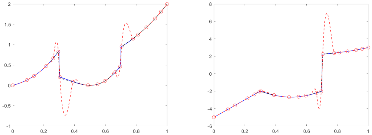
In our second experiment, we only performed a comparison between the presented $PPH$ subdivision scheme and the classical linear scheme with four points based on Lagrange interpolation. We plotted in Figure 1 the subdivision curve obtained for both methods, PPH and Lagrange, after $k=5$ levels of subdivision and starting from the nonuniform grid $X_1$ with 30 initial points used in the first numerical experiment and the associated point values of the function $f\left(x\right).$ The original function is also provided to compare the approximation capabilities of both subdivision methods. We see the original function in a solid blue line, the Lagrange subdivision scheme in a dashed red line, and the PPH subdivision scheme in a dash-dotted black line. As it can be appreciated in Figure 1, the Gibbs effects and undesirable oscillations due to the presence of a jump discontinuity are highly reduced with the PPH scheme in contrast with what happens with the linear scheme. Notice the high oscillations that appear near the jump discontinuities when using the linear scheme, which is known to happen when one implements any linear scheme. In Figure 1, to the right, we show a zoom of the area around the first jump discontinuity to observe more clearly the behavior of the nonlinear scheme. In Figure 2, we also plot the results obtained with the nonuniform grid $X_2$ with 20 non-equally spaced points considered in the previous experiment. We considered both functions $f\left(x\right)$ and $g\left(x\right).$ Again, the same type of Gibbs effects appear around the jump discontinuity for the linear method. The corner is not so problematic.

Figure 2. Comparison of the subdivision curve after $k=5$ subdivision levels for the Lagrange subdivision scheme in a dashed red line and the PPH subdivision scheme in a dash-dotted black line. The original function is also plotted in a solid blue line. The initial control points, plotted with red circles, come from one of the nonuniform grids X considered in our two experiments, the one that consists of 20 abscissas in the interval $[0,1].$ (Left) Subdivision curve for data coming from $f\left(x\right).$ (Right) Subdivision curve for data coming from $g\left(x\right).$

In Table 4, we see the errors $||f^k-{\mathcal{S}}^k{f}^0{||}_p,p=1,2,\infty ,$ committed by approximating the original data $f^k,$ i.e., the right point-values of the function $f\left(x\right)$ at the corresponding abscissas with ${\mathcal{S}}^k{f}^0$ for $k=5$ subdivision levels, where ${\mathcal{S}}^k{f}^0$ stands for the iterative application k times of the analyzed subdivision schemes, namely PPH and Lagrange, starting from the initial function point values $f^0$ at the given grid $X_1$ with 30 abscissae. In Table 5, we give the corresponding results for the grid $X_2$ with 20 abscissae. In Table 6, we consider this time to be the errors $||g^k-{\mathcal{S}}^k{g}^0{||}_p,p=1,2,\infty ,$ for the function $g\left(x\right)$ using the grid $X_2$ with 20 abscissae.

Table 4. Subdivision errors $\left|\right|f^k-{\mathcal{S}}^k{f}^0{\left|\right|}_p,p=1,2,\infty ,$ committed by approximating the original data $f^k$ with ${\mathcal{S}}^k{f}^0$ for $k=5$ subdivision levels starting from the initial function point values $f^0$ at the given grid $X_1$ with 30 points.

Method	$\left|\right|{\mathit{f}}^{\mathit{k}}-{\mathcal{S}}^{\mathit{k}}{\mathit{f}}^0{\left|\right|}_1$	$\left|\right|{\mathit{f}}^{\mathit{k}}-{\mathcal{S}}^{\mathit{k}}{\mathit{f}}^0{\left|\right|}_2$	$\left|\right|{\mathit{f}}^{\mathit{k}}-{\mathcal{S}}^{\mathit{k}}{\mathit{f}}^0{\left|\right|}_{\mathit{\infty }}$
PPH	$0.0098$	$0.0454$	$0.4239$
Lagrange	$0.0388$	$0.1355$	$0.9767$

Table 5. Subdivision errors $\left|\right|f^k-{\mathcal{S}}^k{f}^0{\left|\right|}_p,p=1,2,\infty ,$ committed by approximating the original data $f^k$ with ${\mathcal{S}}^k{f}^0$ for $k=5$ subdivision levels starting from the initial function point values $f^0$ at the given grid $X_2$ with 20 abscissae.

Method	$\left|\right|{\mathit{f}}^{\mathit{k}}-{\mathcal{S}}^{\mathit{k}}{\mathit{f}}^0{\left|\right|}_1$	$\left|\right|{\mathit{f}}^{\mathit{k}}-{\mathcal{S}}^{\mathit{k}}{\mathit{f}}^0{\left|\right|}_2$	$\left|\right|{\mathit{f}}^{\mathit{k}}-{\mathcal{S}}^{\mathit{k}}{\mathit{f}}^0{\left|\right|}_{\mathit{\infty }}$
PPH	$0.0163$	$0.0529$	$0.3412$
Lagrange	$0.0809$	$0.1849$	$0.8953$

Table 6. Subdivision errors $\left|\right|g^k-{\mathcal{S}}^k{g}^0{\left|\right|}_p,p=1,2,\infty ,$ committed by approximating the original data $g^k$ with ${\mathcal{S}}^k{g}^0$ for $k=5$ subdivision levels starting from the initial function point values $g^0$ at the given grid $X_2$ with 20 abscissae.

Method	$\left|\right|{\mathit{f}}^{\mathit{k}}-{\mathcal{S}}^{\mathit{k}}{\mathit{f}}^0{\left|\right|}_1$	$\left|\right|{\mathit{f}}^{\mathit{k}}-{\mathcal{S}}^{\mathit{k}}{\mathit{f}}^0{\left|\right|}_2$	$\left|\right|{\mathit{f}}^{\mathit{k}}-{\mathcal{S}}^{\mathit{k}}{\mathit{f}}^0{\left|\right|}_{\mathit{\infty }}$
PPH	$0.0580$	$0.2808$	$2.1087$
Lagrange	$0.2837$	$0.8468$	$4.6606$

7. Conclusions

We defined and analyzed the PPH subdivision scheme on nonuniform grids, which were derived from its associated reconstruction operator. We paid special attention to the case of $\sigma$ quasi-uniform grids and initial data coming from strictly convex (concave) smooth functions.

We theoretically proved some crucial issues when dealing with subdivision schemes, such as the existence of a contractive scheme for the first differences, convergence, smoothness of the limit function, and preservation of the convexity properties of the initial data.

In the numerical experiments section, we carried out some experiments that reinforce the theoretical results, in particular, we observed the Hölder continuity of the limit function, giving a numerical estimation of the exponent $\alpha$ that coincides with the result in Theorem 2. We also carried out another experiment to analyze the performance of the subdivision scheme with initial data that contain a numerical jump discontinuity, observing that Gibbs effects and oscillations are negligible. Finally, a potential real application in $2D$ was given by zooming in on some coarse data from geological areas corresponding to unaccessible seabeds.

References

1. Amat, S.; Donat, R.; Liandrat, J.; Trillo, J.C. Analysis of a new nonlinear subdivision scheme. Applications in image processing. Found. Comput. Math. 2006, 6, 193–225. [Google Scholar] [CrossRef]
2. Aràndiga, F.; Donat, R. Nonlinear Multi-scale Decomposition: The Approach of A.Harten. Numer. Algorithms 2000, 23, 175–216. [Google Scholar] [CrossRef]
3. Harten, A. Multiresolution representation of data II. SIAM J. Numer. Anal. 1996, 33, 1205–1256. [Google Scholar] [CrossRef]
4. Amat, S.; Ruiz, J.; Trillo, J.C.; Yáñez, D.F. On a family of non-oscillatory subdivision schemes having regularity Cr with r > 1. Numer. Algorithms 2020, 85, 543–569. [Google Scholar] [CrossRef]
5. Donat, R.; López Ureña, S. Nonlinear stationary subdivision schemes reproducing hyperbolic and trigonometric functions. Adv. Comput. Math. 2019, 45, 3137–3172. [Google Scholar] [CrossRef]
6. Dyn, N.; Levin, D.; Massopust, P. Attractors of trees of maps and of sequences of maps between spaces with applications to subdivision. J. Fixed Point Theory Appl. 2020, 22, 24. [Google Scholar] [CrossRef]
7. Levin, D.; Dyn, N.; Viswanathan, P.V. Non-stationary versions of fixed-point theory, with applications to fractals and subdivision. J. Fixed Point Theory Appl. 2019, 21, 26. [Google Scholar] [CrossRef]
8. Moosmüller, C.; Dyn, N. Increasing the smoothness of vector and Hermite subdivision schemes. IMA J. Numer. Anal. 2019, 39, 579–606. [Google Scholar] [CrossRef] [Green Version]
9. Amat, S.; Donat, R.; Trillo, J.C. Proving convexity preserving properties of interpolatory subdivision schemes through reconstruction operators. Appl. Math. Comput. 2013, 219, 7413–7421. [Google Scholar] [CrossRef]
10. Floater, M.S.; Michelli, C.A. Nonlinear Stationary Subdivision. Approx. Theory 1998, 212, 209–224. [Google Scholar]
11. Ortiz, P.; Trillo, J.C. On the convexity preservation of a quasi C3 nonlinear interpolatory reconstruction operator on σ quasi-uniform grids. Mathematics 2021, 9, 310. [Google Scholar] [CrossRef]
12. Ortiz, P.; Trillo, J.C. PPH nonlinear interpolatory reconstruction operator on non uniform grids: Adaptation around jump discontinuities and elimination of Gibbs phenomenon. Mathematics 2021, 9, 335. [Google Scholar] [CrossRef]