
A Low Dissipative and Stable Cell-Centered Finite Volume Method with the Simultaneous Approximation Term for Compressible Turbulent Flows


Abstract
1. Introduction
2. Governing Equations and Turbulence Modeling
2.1. Unfiltered Navier–Stokes Equations
2.2. Spatially Filtered Navier–Stokes Equations
2.3. Subgrid-Scale Modeling
3. Numerical Methods, Verification, and Validation
3.1. Two-Dimensional Propagating Inviscid Vortex
3.2. LES of Supersonic Turbulent Channel Flow
4. Simultaneous Approximation Term
4.1. SBP–SAT Approach
4.2. NSBP–SAT Approach for a Cell-Centered Finite-Volume Method
4.3. Two-Dimensional Acoustic Pulse
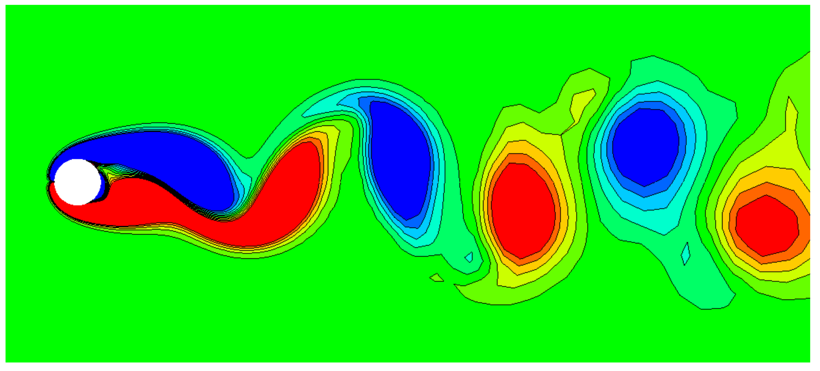
4.4. Low Reynolds Number Flow around a Two-Dimensional Circular Cylinder
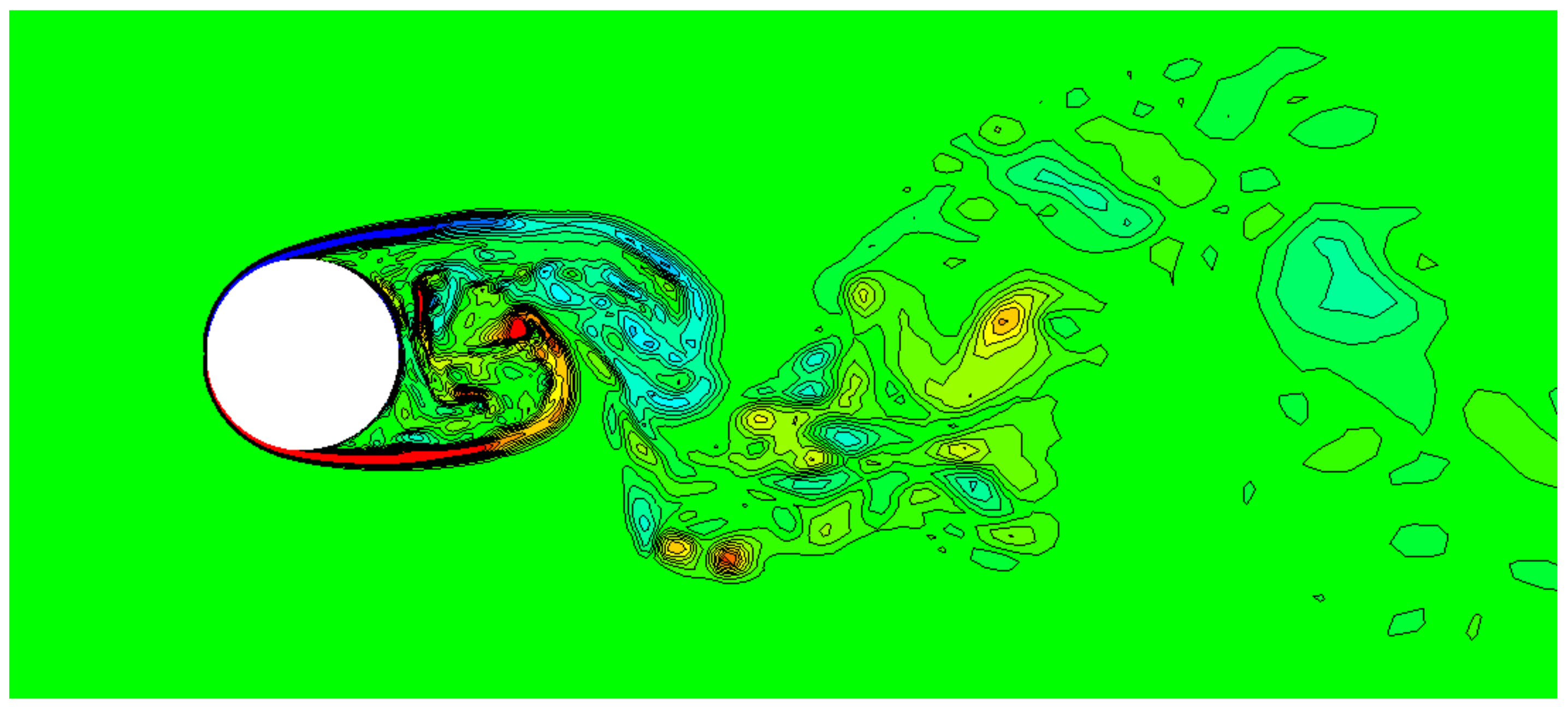
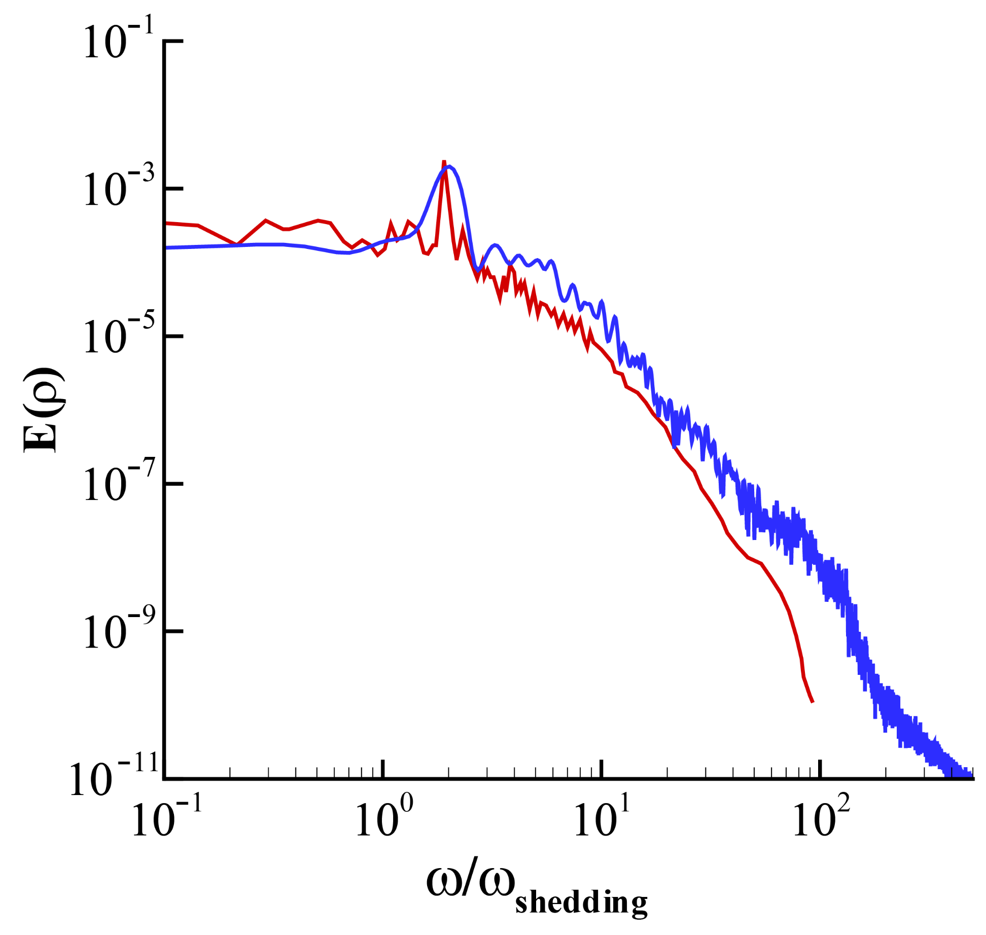
4.5. LES of Flow over a Circular Cylinder at M = 0.4
5. Comparative Study of the SAT and the CBC
5.1. Description of the Characteristic Boundary Condition
5.2. Characteristic Boundary Condition for a Cell-Centered FVM
5.3. Convecting Two-Dimensional Inviscid Vortex
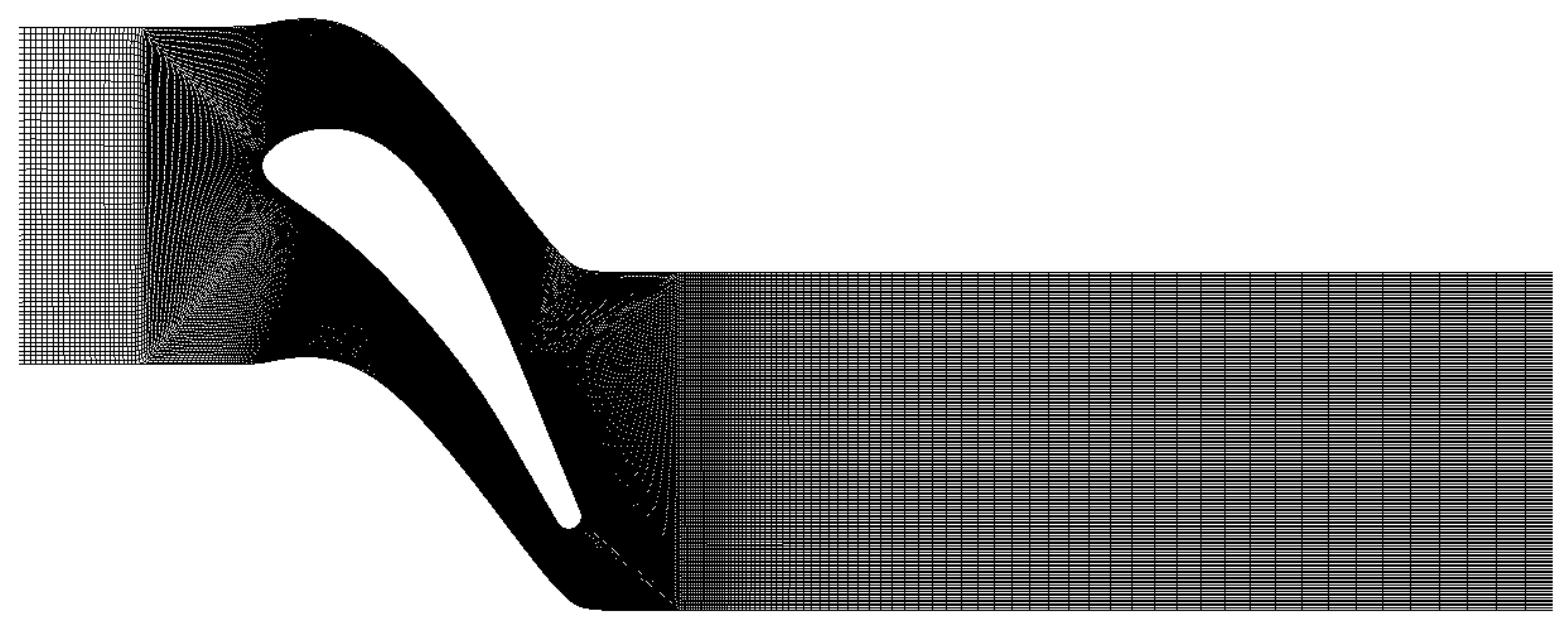
5.4. LES of Flow through the VKI Subsonic Turbine Cascade
6. Concluding Remarks
Author Contributions
Funding
Institutional Review Board Statement
Informed Consent Statement
Data Availability Statement
Conflicts of Interest
Abbreviations
| CBC | Characteristic boundary condition |
| DNS | Direct numerical simulation |
| ENO | Essentially non-oscillatory |
| EOCBC | Extrapolated original characteristic boundary condition |
| FDM | Finite-difference method |
| FVM | Finite-volume method |
| GBCBC | Gradient-based characteristic boundary condition |
| HLLC | Harten–Lax-van Leer–Contact |
| LES | Large eddy simulation |
| RMS | Root mean square |
| SAT | Simultaneous approximation term |
| SBP | Summation by parts |
| SGS | Subgrid scale |
| VKI | von Karman Institute for Fluid Dynamics |
References
- Mittal, R.; Moin, P. Suitability of upwind-biased finite difference schemes for large-eddy simulation of turbulent flows. AIAA J. 1997, 35, 1415–1417. [Google Scholar] [CrossRef]
- Poinsot, T.J.A.; Lele, S.K. Boundary conditions for direct simulations of compressible viscous flows. J. Comput. Phys. 1992, 101, 104–129. [Google Scholar] [CrossRef]
- Carpenter, M.H.; Gottlieb, D.; Abarbanel, S. Time-stable boundary conditions for finite-difference schemes solving hyperbolic systems: Methodology and application to high-order compact schemes. J. Comput. Phys. 1994, 111, 220–236. [Google Scholar] [CrossRef]
- Svärd, M.; Carpenter, M.H.; Nordström, J. A stable high-order finite difference scheme for the compressible Navier–Stokes equations, far-field boundary conditions. J. Comput. Phys. 2007, 225, 1020–1038. [Google Scholar] [CrossRef]
- Svärd, M.; Nordström, J. Review of summation-by-parts schemes for initial–boundary-value problems. J. Comput. Phys. 2014, 268, 17–38. [Google Scholar] [CrossRef]
- Fernández, D.C.D.R.; Hicken, J.E.; Zingg, D.W. Review of summation-by-parts operators with simultaneous approximation terms for the numerical solution of partial differential equations. Comput. Fluids 2014, 95, 171–196. [Google Scholar] [CrossRef]
- Nordström, J.; Forsberg, K.; Adamsson, C.; Eliasson, P. Finite volume methods, unstructured meshes and strict stability for hyperbolic problems. Appl. Numer. Math. 2003, 45, 453–473. [Google Scholar] [CrossRef]
- Shoeybi, M.; Svärd, M.; Ham, F.E.; Moin, P. An adaptive implicit–explicit scheme for the DNS and LES of compressible flows on unstructured grids. J. Comput. Phys. 2010, 229, 5944–5965. [Google Scholar] [CrossRef]
- Nordström, J.; Björck, M. Finite volume approximations and strict stability for hyperbolic problems. Appl. Numer. Math. 2001, 38, 237–255. [Google Scholar] [CrossRef]
- Khalighi, Y.; Ham, F.; Nichols, J.; Lele, S.; Moin, P. Unstructured large eddy simulation for prediction of noise issued from turbulent jets in various configurations. In Proceedings of the 17th AIAA/CEAS Aeroacoustics Conference (32nd AIAA Aeroacoustics Conference), Portland, OR, USA, 5 June–8 June 2011. AIAA 2011-2886. [Google Scholar]
- Peterson, D.M. Simulations of Injection, Mixing, and Combustion in Supersonic Flow Using a Hybrid RANS/LES Approach. Ph.D. Thesis, University of Minnesota, Minneapolis, MN, USA, 2011. [Google Scholar]
- Ma, P.C.; Lv, Y.; Ihme, M. An entropy-stable hybrid scheme for simulations of transcritical real-fluid flows. J. Comput. Phys. 2017, 340, 330–357. [Google Scholar] [CrossRef]
- Toro, E.F.; Spruce, M.; Speares, W. Restoration of the contact surface in the HLL-Riemann solver. Shock Waves 1994, 4, 25–34. [Google Scholar] [CrossRef]
- Garnier, E.; Adams, N.; Sagaut, P. Large Eddy Simulation for Compressible Flows; Springer Science & Business Media: Dordrecht, The Netherlands, 2009; pp. 6–8. [Google Scholar]
- Pope, S.B. Turbulent Flows; Cambridge University Press: Cambridge, UK, 2012; pp. 344–357. [Google Scholar]
- Deardorff, J.W. A numerical study of three-dimensional turbulent channel flow at large Reynolds numbers. J. Fluid Mech. 1970, 41, 453–480. [Google Scholar] [CrossRef]
- Okong’o, N.A.; Bellan, J. Consistent large-eddy simulation of a temporal mixing layer laden with evaporating drops. Part 1. Direct numerical simulation, formulation and a priori analysis. J. Fluid Mech. 2004, 499, 1–47. [Google Scholar] [CrossRef]
- Yoshizawa, A. Statistical theory for compressible turbulent shear flows, with the application to subgrid modeling. Phys. Fluids 1986, 29, 2152–2164. [Google Scholar] [CrossRef]
- Vreman, A.W. An eddy-viscosity subgrid-scale model for turbulent shear flow: Algebraic theory and applications. Phys. Fluids 2004, 16, 3670–3681. [Google Scholar] [CrossRef]
- Shu, C.W.; Osher, S. Efficient implementation of essentially non-oscillatory shock-capturing schemes. J. Comput. Phys. 1988, 77, 439–471. [Google Scholar] [CrossRef]
- Tucker, P.G. Novel MILES computations for jet flows and noise. Int. J. Heat Fluid Flow 2004, 25, 625–635. [Google Scholar] [CrossRef]
- Shur, M.L.; Spalart, P.R.; Strelets, M.K.; Travin, A.K. Towards the prediction of noise from jet engines. Int. J. Heat Fluid Flow 2003, 24, 551–561. [Google Scholar] [CrossRef]
- Xia, H.; Tucker, P.G.; Eastwood, S. Large-eddy simulations of chevron jet flows with noise predictions. Int. J. Heat Fluid Flow 2009, 30, 1067–1079. [Google Scholar] [CrossRef]
- Le, H.; Moin, P. An improvement of fractional step methods for the incompressible Navier-Stokes equations. J. Comput. Phys. 1991, 92, 369–379. [Google Scholar] [CrossRef]
- Lenormand, E.; Sagaut, P.; Phuoc, L.T.; Comte, P. Subgrid-scale models for large-eddy simulations of compressible wall bounded flows. AIAA J. 2000, 38, 1340–1350. [Google Scholar] [CrossRef]
- Moin, P.; Squires, K.; Cabot, W.; Lee, S. A dynamic subgrid-scale model for compressible turbulence and scalar transport. Phys. Fluids 1991, 3, 2746–2757. [Google Scholar] [CrossRef]
- Coleman, G.N.; Kim, J.; Moser, R.D. A numerical study of turbulent supersonic isothermal-wall channel flow. J. Fluid Mech. 1995, 305, 159–184. [Google Scholar] [CrossRef]
- Silvis, M.H.; Remmerswaal, R.A.; Verstappen, R. Physical consistency of subgrid-scale models for large-eddy simulation of incompressible turbulent flows. Phys. Fluids 2017, 29, 015105. [Google Scholar] [CrossRef]
- Shoeybi, M. A Hybrid Implicit-Explicit Method for the LES of Compressible Flows on Unstructured Grids. Ph.D. Thesis, Stanford University, Stanford, CA, USA, 2010. [Google Scholar]
- Svärd, M.; Nordström, J. A stable high-order finite difference scheme for the compressible Navier–Stokes equations: No-slip wall boundary conditions. J. Comput. Phys. 2008, 227, 4805–4824. [Google Scholar] [CrossRef]
- Fey, U.; König, M.; Eckelmann, H. A new Strouhal–Reynolds-number relationship for the circular cylinder in the range 47 < Re < 2 × 10⁵. Phys. Fluids 1998, 10, 1547–1549. [Google Scholar]
- Bodony, D.J. Analysis of sponge zones for computational fluid mechanics. J. Comput. Phys. 2006, 212, 681–702. [Google Scholar] [CrossRef]
- Mani, A.; Moin, P.; Wang, M. Computational study of optical distortions by separated shear layers and turbulent wakes. J. Fluid Mech. 2009, 625, 273–298. [Google Scholar] [CrossRef]
- Nagarajan, S.; Lele, S.K.; Ferziger, J.H. A robust high-order compact method for large eddy simulation. J. Comput. Phys. 2003, 191, 392–419. [Google Scholar] [CrossRef]
- Sayadi, T.; Moin, P. Large eddy simulation of controlled transition to turbulence. Phys. Fluids 2012, 24, 114103. [Google Scholar] [CrossRef]
- Kravchenko, A.G.; Moin, P. Numerical studies of flow over a circular cylinder at ReD = 3900. Phys. Fluids 2000, 12, 403–417. [Google Scholar] [CrossRef]
- Sagaut, P. Large Eddy Simulation for Incompressible Flows: An Introduction; Springer Science & Business Media: Berlin, Germany, 2006; p. 19. [Google Scholar]
- Thompson, K.W. Time dependent boundary conditions for hyperbolic systems. J. Comput. Phys. 1987, 68, 1–24. [Google Scholar] [CrossRef]
- Yoo, C.S.; Wang, Y.; Trouvé, A.; Im, H.G. Characteristic boundary conditions for direct simulations of turbulent counterflow flames. Combust. Theory Model. 2005, 9, 617–646. [Google Scholar] [CrossRef]
- Gross, A.; Fasel, H.F. Characteristic ghost cell boundary condition. AIAA J. 2007, 45, 302–306. [Google Scholar] [CrossRef]
- Motheau, E.; Almgren, A.; Bell, J.B. Navier–Stokes characteristic boundary conditions using ghost cells. AIAA J. 2017, 55, 3399–3408. [Google Scholar] [CrossRef]
- Kang, M.; You, D. Study of a non-reflecting characteristic boundary condition for compressible flow simulation using a cell-centered finite-volume method. J. Comput. Fluid. Eng. 2020, 25, 123–134. [Google Scholar] [CrossRef]
- Prosser, R. Improved boundary conditions for the direct numerical simulation of turbulent subsonic flows. I. Inviscid flows. J. Comput. Phys. 2005, 207, 736–768. [Google Scholar] [CrossRef]
- Lodato, G.; Domingo, P.; Vervisch, L. Three-dimensional boundary conditions for direct and large-eddy simulation of compressible viscous flows. J. Comput. Phys. 2008, 227, 5105–5143. [Google Scholar] [CrossRef]
- Granet, V.; Vermorel, O.; Léonard, T.; Gicquel, L.; Poinsot, T. Comparison of nonreflecting outlet boundary conditions for compressible solvers on unstructured grids. AIAA J. 2010, 48, 2348–2364. [Google Scholar] [CrossRef]
- Dixon, S.L.; Hall, C. Fluid Mechanics and Thermodynamics of Turbomachinery; Butterworth-Heinemann: Oxford, UK, 2013; pp. 22, 27. [Google Scholar]
- Hah, C. Large eddy simulation of transonic flow field in NASA rotor 37. In Proceedings of the 47th AIAA Aerospace Sciences Meeting Including the New Horizons Forum and Aerospace Exposition, Orlando, FL, USA, 5–8 January 2009. [Google Scholar]
- Eppler, R. Airfoil Design and Data; Springer Science & Business Media: Berlin, Germany, 2012; pp. 81, 140. [Google Scholar]
- Sieverding, C.H.; Richard, H.; Desse, J.M. Turbine blade trailing edge flow characteristics at high subsonic outlet Mach number. J. Turbomach. 2003, 125, 298–309. [Google Scholar] [CrossRef]
- Magagnato, F.; Pritz, B.; Gabi, M. Generation of inflow conditions for large-eddy simulation of compressible flows. In Proceedings of the 8th International Symposium on Experimental and Computational Aerothermodynamics of Internal Flows, Lyon, France, 2 July–6 July 2007. [Google Scholar]
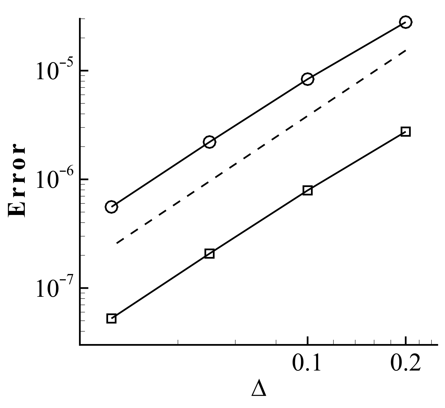
 , second-order convergence.
, second-order convergence.
, second-order convergence.
 , LES with cells;
  , LES with cells.
, LES with cells; , LES with cells.
, LES with cells.
, LES with cells; , LES with cells.


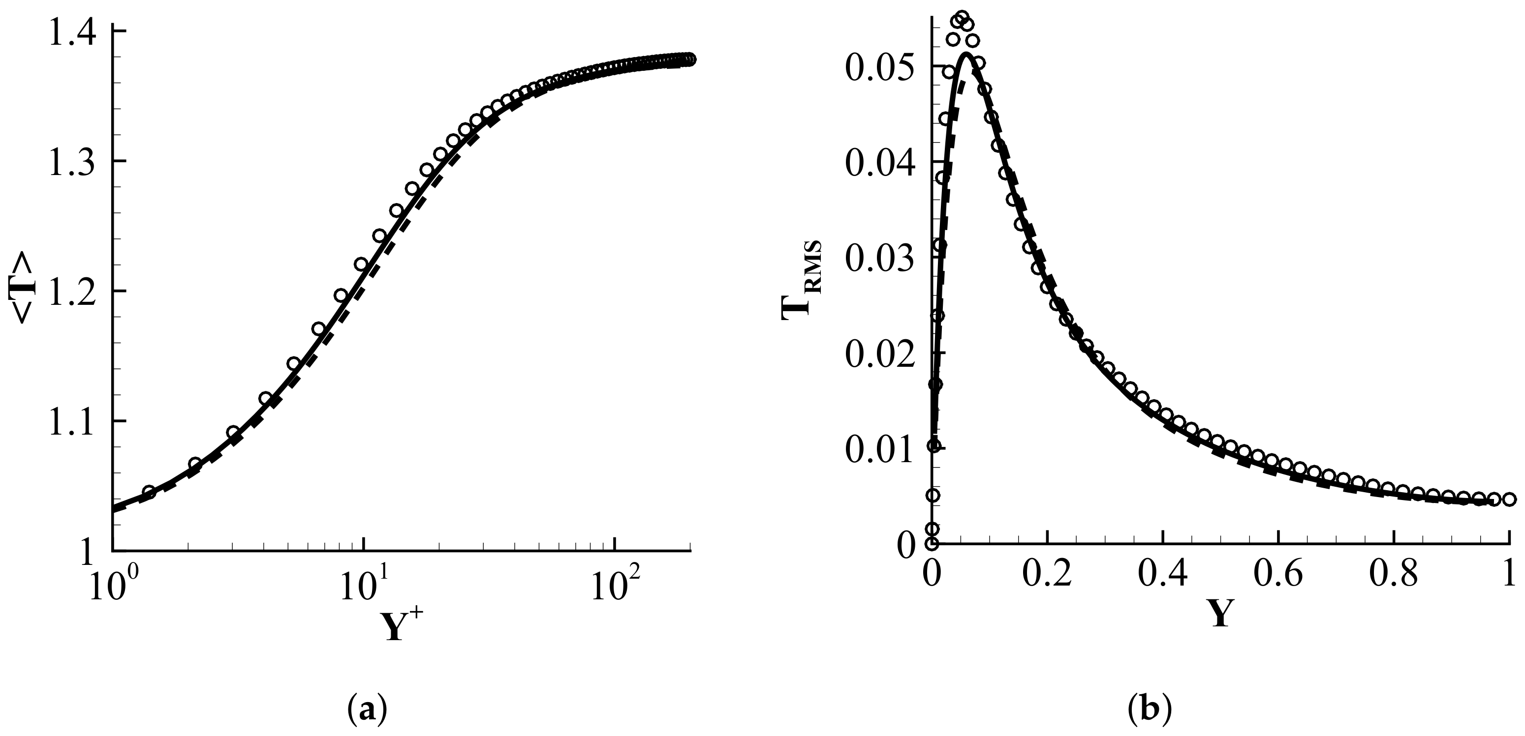
 , the present LES;
  , LES by Mani et al. [33].
, the present LES; , LES by Mani et al. [33].
, LES by Mani et al. [33].
, the present LES; , LES by Mani et al. [33].


| Average | Max. | Min. | ||
|---|---|---|---|---|
| Coarse-grid case | 1.346 | 0.3249 | −0.3249 | 0.167 |
| Fine-grid case | 1.344 | 0.3258 | −0.3258 | 0.167 |
| Svärd and Nordström [30] | 1.341 | 0.3268 | −0.3268 | 0.165 |
| Shoeybi et al. [8] | 1.347 | 0.168 | ||
| Fey et al. [31] | 0.165 ± 0.001 |
| Average | ||
|---|---|---|
| Present results | ||
| Mani et al. [33] |
Publisher’s Note: MDPI stays neutral with regard to jurisdictional claims in published maps and institutional affiliations. |
© 2021 by the authors. Licensee MDPI, Basel, Switzerland. This article is an open access article distributed under the terms and conditions of the Creative Commons Attribution (CC BY) license (https://creativecommons.org/licenses/by/4.0/).
Share and Cite
Kang, M.; You, D. A Low Dissipative and Stable Cell-Centered Finite Volume Method with the Simultaneous Approximation Term for Compressible Turbulent Flows. Mathematics 2021, 9, 1206. https://doi.org/10.3390/math9111206
Kang M, You D. A Low Dissipative and Stable Cell-Centered Finite Volume Method with the Simultaneous Approximation Term for Compressible Turbulent Flows. Mathematics. 2021; 9(11):1206. https://doi.org/10.3390/math9111206
Chicago/Turabian StyleKang, Myeongseok, and Donghyun You. 2021. "A Low Dissipative and Stable Cell-Centered Finite Volume Method with the Simultaneous Approximation Term for Compressible Turbulent Flows" Mathematics 9, no. 11: 1206. https://doi.org/10.3390/math9111206
APA StyleKang, M., & You, D. (2021). A Low Dissipative and Stable Cell-Centered Finite Volume Method with the Simultaneous Approximation Term for Compressible Turbulent Flows. Mathematics, 9(11), 1206. https://doi.org/10.3390/math9111206