Variational Fusion of Hyperspectral Data by Non-Local Filtering

Abstract

The fusion of multisensor data has attracted a lot of attention in computer vision, particularly among the remote sensing community. Hyperspectral image fusion consists in merging the spectral information of a hyperspectral image with the geometry of a multispectral one in order to infer an image with high spatial and spectral resolutions. In this paper, we propose a variational fusion model with a nonlocal regularization term that encodes patch-based filtering conditioned to the geometry of the multispectral data. We further incorporate a radiometric constraint that injects the high frequencies of the scene into the fused product with a band per band modulation according to the energy levels of the multispectral and hyperspectral images. The proposed approach proved robust to noise and aliasing. The experimental results demonstrate the performance of our method with respect to the state-of-the-art techniques on data acquired by commercial hyperspectral cameras and Earth observation satellites.

1. Introduction

Image fusion has been an active field of research due to the growing availability of data and the need of gathering information from different imaging sources [1,2]. In this setting, merging multisensor data in general and images with different spatial and spectral resolutions in particular has attracted a lot of attention in computer vision.

Hyperspectral (HS) imaging describes and characterizes the Earth surface components and processes thanks to the measurements of the interaction of light with objects, which is called spectral response. Everyday-life scenes captured by HS cameras [3] are used in many computer vision tasks such as recognition or surveillance. Furthermore, remote sensing HS data delivered by satellites through various missions help shed more light on many Earth phenomena [4,5].

Imaging sensor performances are mainly assessed with the Ground Sampling Distance (GSD) factor and the number of spectral bands. Lower GSD provides images with good spatial quality, while a higher number of spectral bands allows better spectral description of the captured scene. However, imaging sensors are subject to compromises due to various technical and economical constraints. For instance, the compromise between the GSD and the signal to noise ratio (SNR) is taken into account in order to maintain low-level noise in the images. The bandwidth capacity as well as the onboard storage are important limiting factors too. These tradeoffs lead to acquiring a multispectral (MS) image with high spatial but low spectral resolution, or an HS image with accurate spectral but poorer spatial resolution. Such a scenario opens the gate to fusion [6] and to super-resolution techniques [7,8].

Hyperspectral image fusion consists in merging the spectral information of an HS image with the geometry of an MS image in order to infer an image with high spatial and spectral resolutions. Since the fusion problem is generally ill posed, some state-of-the-art methods introduce prior knowledge through the Bayesian [9,10] or variational [11,12] frameworks. Other approaches associate fusion with super-resolution [13] or linear spectral unmixing [14]. With the increased prominence of deep learning, convolutional neural networks (CNNs) have been recently used [15,16].

A closely related problem to HS fusion is pansharpening [17,18]. The difference between the two is not only that the geometry is encoded in a grayscale image in the case of pansharpening, but also that the number of spectral bands to be spatially interpolated is much lower than in HS fusion. Nonetheless, pansharpening models can be well adapted to the fusion of HS and MS images [19].

In this paper, we propose to tackle HS fusion in the variational framework through the minimization of a convex energy. In order to deal with the ill-posed nature of the problem, we incorporate a nonlocal regularization term that encodes patch-based filtering conditioned to the geometry of the MS image. A radiometric constraint is also introduced in order to inject the high frequencies of the scene into the fused product with a band per band modulation according to the energy levels of the MS and HS images. The proposed model is compared with several state-of-the art techniques on both remote sensing imagery and data captured by HS cameras of everyday-life scenes. An ablation study on modules of our method is also included. This work extends our previous conference paper [20], which contains very preliminary results. By contrast, in this work we include additional and extensive analysis of the proposed fusion model. More specifically, we apply the saddle-point formulation and the primal dual scheme for solving the proposed variational model and we validate our fusion technique with a variety of experiments on different types of HS data.

The rest of the paper is organized as follows. In Section 2, we review the state of the art in HS fusion. Section 3 details the proposed variational model, while its robustness to different phenomena is analyzed in Section 4. The performance of the method is exhaustively evaluated in Section 5. Finally, conclusions are drawn in Section 6.

2. State of the Art

In this section, we outline the state of the art in HS fusion. For detailed surveys, we refer to [6,21].

Pansharpening has been widely used to enhance the spatial resolution of MS imagery by fusing MS data with a higher-resolution panchromatic image [17,18]. With the growing number of HS sensors, many methods throughout the literature adapted pansharpening to HS fusion. The first proposals in this direction were based on wavelets [22,23], but the quality of the fusion depends on the way MS data is interpolated in the spectral domain. Chen et al. [19] divided the spectrum of the HS image into many regions and applied a pansharpening algorithm in each one. Selva et al. [24] introduced hypersharpening, according to which each HS band is synthesized as a linear combination of the MS bands in order to produce a high-resolution image. The method is tested on the base of generalized Laplacian pyramid (GLP) [25]. Other classical pansharpening approaches such as Gram-Schmidt adaptive (GSA) [26] and smoothing filtered-based intensity modulation (SFIM) [27] have also been adapted to HS fusion [6].

The fusion problem is an ill-posed one, therefore, some state-of-the-art methods introduce prior knowledge on the image to be found based on various frameworks but usually within the variational or Bayesian one. Ballester et al. [28] were the first to introduce a variational formulation for pansharpening. The authors assumed that the low-resolution channels are a low-passed and downsampled version of the high-resolution ones. Then, they imposed a regularization term forces the edges of each spectral band to line up with those of the panchromatic one. Duran et al. [29] kept the same variational formulation and incorporated nonlocal regularization to harness the self-similarities in the panchromatic image. Posteriorly, the same authors [18] introduced a new constraint imposing the preservation of the radiometric ratio between the panchromatic image and each spectral band and obtained a model with no assumption on the co-registration of the spectral data. In the Bayesian setting, Fasbender et al. [30] pioneered a Bayesian fusion method that relies on statistical relationships between the MS bands and the panchromatic one without restrictive modeling hypotheses.

As in pansharpening, the HS fusion problem can be tackled in the variational framework. Wei et al. [12] proposed a variational fusion approach with a sparse regularization term that is determined based on the decomposition of the scene on a set of dictionaries. Simoes et al. [11] combined a total variation based regularization with two quadratic data-fitting terms accounting for blur, downsampling and noise. The authors also explored inherent redundancies within the images with data reduction techniques. Zhang et al. [31] presented a group spectral embedding fusion method exploring the multiple manifold structures of spectral bands and the low-rank structure of HS images. Bungert et al. [32] proposed a variational model for simultaneous image fusion and blind deblurring of HS images based on the directional total variation. Mifdal et al. [33] pioneered an optimal transport technique that models the fusion problem as the minimization of the sum of two regularized Wasserstein distances. However, the noise was not taken into account, therefore, a pre-processing step for the denoising of HS and MS data is required.

In the Bayesian setting, HS fusion methods integrate prior knowledge and posterior distribution on the data. Eismann and Hardie [9,10] developed a Bayesian method based on a maximum a posteriori estimation and a stochastic mixing model of the spectral scene (MAPMM). The aim of these estimations is to develop a cost function that optimizes the target image. Wei et al.  [34] designed a hierarchical Bayesian model with a prior distribution that exploits geometrical concepts encountered in spectral unmixing problems. The resulting posterior distribution is sampled using a Hamiltonian Monte Carlo algorithm. The same authors proposed in [35] a Sylvester equation-based fusion model, which they named FUSE, that allows the use of Bayesian estimators.

In hyperspectral imaging, each pixel is considered to be a mixture of various distinct materials (grass, road, cars, etc.) with certain proportions. The materials are represented in a matrix called endmembers and the propotions are stored in a abundance matrix. The unmixing method [36,37] for HS fusion is based on spectra separation techniques. In this setting, endmembers and abundance matrices are obtained from HS and MS data and the fused image is assumed to be the product of both matrices. Berné et al. [38] suggested a fusion method based on the decomposition of the HS data using non-negative matrix factorization (NMF). In [39], the spatial sparsity of the HS data was harnessed and only a few materials were assumed to constitute the composition of a pixel in the HS image. Yokoya et al. [14] presented an approach where HS and MS data are alternately unmixed to extract the endmember and abundance matrices, while Akhtar et al. [8] used dictionary learning for the estimation of such matrices. Finally, Lanaras et al. [40] introduced a linear mixing model for HS fusion which is solved with a projected gradient scheme.

Recently, deep learning and especially CNNs have been enjoying a huge success in many applications in the image processing field. CNNs models are composed of layers where convolution-based operations take place. Many deep architectures for super-resolution [41,42] and fusion methods [15,16,43] have been proposed so far. Palsson et al. [15] introduced a 3D CNN for HS fusion. In order to reduce the computational cost and make the method robust to noise, the authors reduced he dimensionality of the HS image before the fusion process. In [16], the authors presented a deep CNN with two branches devoted to HS and MS image features, respectively. Once the features are extracted, they are concatenated and put through the fully connected layers that provide as output the spectrum of the expected fused image. Xie et al. [43] constructed a model-based deep learning approach that harness the data generation model and the low-rankness along the spectral mode of the unknown image. Then, a deep network is designed to learn the proximal operator and model parameters. Recently, Dian et al. [44] suggested a CNN denoiser to regularize the fusion of HS and MS images. First, the high-resolution HS image is decomposed into subspace and coefficients. The subspace is learnt from the HS image using the singular value decomposition (SVD). Finally, a CNN trained for the denoising of gray images is used to regularize the estimation of coefficients with the use of the alternating direction method of multipliers (ADMM) algorithm.

3. Variational HS Fusion Method

In this section, we introduce a nonlocal variational HS fusion model. In addition to the classical data-fitting terms that penalize deviations from the generation models of MS and HS data, we incorporate nonlocal regularization conditioned to the geometry of the MS image and a radiometric constraint that introduces high frequencies of the captured scene into the fused image.

We assume that any single-channel image is given in a regular Cartesian grid and then rasterized by rows in a vector of length equal to the number of pixels. Therefore, the high-resolution HS fused image with H bands and N pixels is denoted by $u={(u_1,\dots ,u_H)}^{\top }\in {\mathbb{R}}^{H\times N}$, where $u_h={(u_h\left(x_1\right),\dots ,u_h\left(x_N\right))}^{\top }\in {\mathbb{R}}^N$ for each $h\in \{1,\dots ,H\}$ and $x_i$ denotes the linearized index of pixel coordinates.

Let $f={(f_1,\dots ,f_M)}^{\top }\in {\mathbb{R}}^{M\times N}$ denote the high-resolution MS image with M spectral bands and N pixels. Similarly, let $g={(g_1,\dots ,g_H)}^{\top }\in {\mathbb{R}}^{H\times N_l}$ be the low-resolution HS image with H spectral bands and $N_l=\frac{N}{l^2}$ pixels. In this setting, $M\ll N$ because of the spectral degradation of f, and $l\in {\mathbb{Z}}^{+}$ is the sampling factor modelling the spatial degradation of g.

For the sake of simplicity, we define the finite-dimensional vector spaces $\mathcal{X}={\mathbb{R}}^{H\times N}$, $\mathcal{Y}={\mathbb{R}}^{H\times N\times N}$, $\mathcal{Z}={\mathbb{R}}^{H\times N_l}$ and $\mathcal{W}={\mathbb{R}}^{M\times N}$ endowed with their standard scalar products. In this setting, we have that $u\in \mathcal{X}$, $g\in \mathcal{Z}$ and $f\in \mathcal{W}$. An element of $\mathcal{Y}$ is written as $p=(p_1,\dots ,p_H)\in \mathcal{Y}$, where $p_h={(p_h\left(x_1\right),\dots ,p_h\left(x_N\right))}^{\top }\in {\mathbb{R}}^{N\times N}$ for each $h\in \{1,\dots ,H\}$ and $p_h\left(x_i\right)={(p_h^1\left(x_i\right),\dots ,p_h^N\left(x_i\right))}^{\top }\in {\mathbb{R}}^N$ for each $i\in \{1,\dots ,N\}$.

The most common data observation models [45] relate the HS and MS data with u by means of

$$\begin{array}{cc}\hfill g_h& =DB{u}_h+{\epsilon }_h,\forall h\in \{1,\dots ,H\},\hfill \\ \hfill f_m& ={\left(Su\right)}_m+{\epsilon }_m,\forall m\in \{1,\dots ,M\},\hfill \end{array}$$

(1)

where B is the low-pass filter that models the point spread function of the HS sensors, D is the downsampling operator, S is the spectral degradation operator representing the responses of the MS sensors, ${\epsilon }_h$ and ${\epsilon }_m$ are the realization of i.i.d. zero-mean band-dependent Gaussian noise. For the sake of simplicity, we consider that B and D are the same for all bands. The operators in (1) can be obtained by registration and radiometric calibration so they are assumed to be known [14]. In the end, the MS image is supposed to be a spectrally degraded noisy version of u, while the HS image is a blurred, downsampled and noisy version of u.

Since recovering u from (1) is an ill-posed inverse problem, the choice of a good prior is required. We tackle it in the variational framework by introducing nonlocal regularization conditioned to the geometry of the MS image. Then, the proposed energy functional is

$$\begin{array}{cc}\hfill & \underset{u\in \mathcal{X}}{min}{\parallel {\nabla }_{\omega }u\parallel }_1+{\displaystyle \frac{\mu }{2}}\sum _{h=1}^H{\parallel DB{u}_h-g_h\parallel }_2^2\hfill \\ \hfill & +{\displaystyle \frac{\gamma }{2}}\sum _{m=1}^M{\parallel \left(Su\right)}_m-f_m{\parallel }_2^2+{\displaystyle \frac{\lambda }{2}}\sum _{h=1}^H{\parallel {\tilde{P}}_h{u}_h-P_h{\tilde{g}}_h\parallel }_2^2,\hfill \end{array}$$

(2)

where $\mu ,\gamma ,\lambda >0$ are trade-off parameters, ${\nabla }_{\omega }$ denotes the nonlocal gradient operator defined in terms of a similarity measure $\omega$, $P\in \mathcal{X}$ is a linear combination of the MS bands, $\tilde{P}\in \mathcal{X}$ is a linear combination of the low frequencies of the MS bands, and $\tilde{g}\in \mathcal{X}$ contains the low frequencies of the HS image in the spatial domain of u. The second and third energy terms are just the variational formulations of the generation models (1). The first term in (2) stands for the nonlocal regularization and the last one for the radiometric constraint. More details are given in next subsections.

3.1. Non-Local Filtering Conditioned to the Geometry of the MS Image

The nonlocal gradient operator ${\nabla }_{\omega }:\mathcal{X}\to \mathcal{Y}$ computes weighted differences between any pair of pixels in terms of a similarity measure $\left\{{\omega }_{h,i,j}\right\}$, with ${\omega }_{h,i,j}={\omega }_h(x_i,x_j)>0$ for $i,j\in \{1,\dots ,N\}$ and $h\in \{1,\dots ,H\}$. Thus, the nonlocal gradient of $u\in \mathcal{X}$ is ${\nabla }_{\omega }u=({\nabla }_{\omega }{u}_1,\dots ,{\nabla }_{\omega }{u}_H)\in \mathcal{Y}$ where ${\nabla }_{\omega }{u}_h={({\nabla }_{\omega }{u}_h\left(x_1\right),\dots ,{\nabla }_{\omega }{u}_h\left(x_N\right))}^{\top }\in {\mathbb{R}}^{N\times N}$ and ${\nabla }_{\omega }{u}_h\left(x_i\right)={({\nabla }_{\omega }{u}_h^1\left(x_i\right),\dots ,{\nabla }_{\omega }{u}_h^N\left(x_i\right))}^{\top }\in {\mathbb{R}}^N$ is a vector containing the weighted differences

$${\nabla }_{\omega }{u}_h^j\left(x_i\right)=\sqrt{{\omega }_{h,i,j}}\left(u_h\left(x_j\right)-u_h\left(x_i\right)\right).$$

(3)

The nonlocal divergence operator ${\mathrm{div}}_{\omega }:\mathcal{Y}\to \mathcal{X}$ is defined by the standard adjoint relation with the nonlocal gradient, that is, ${\langle {\nabla }_{\omega }u,p\rangle }_{\mathcal{Y}}=-{\langle u,{\mathrm{div}}_{\omega }p\rangle }_{\mathcal{X}}$ for every $u\in \mathcal{X}$ and $p\in \mathcal{Y}$. For general non symmetric weights $\omega$, this leads to the following expression:

$${\mathrm{div}}_{\omega }{p}_h\left(x_i\right)=\sum _{j=1}^N\left(p_h^j\left(x_i\right)\sqrt{{\omega }_{h,i,j}}-p_h^i\left(x_j\right)\sqrt{{\omega }_{h,j,i}}\right),$$

(4)

for each $h\in \{1,\dots ,H\}$ and $i\in \{1,\dots ,N\}$. We refer to [29] for a deeper insight on nonlocal vector calculus.

The nonlocal gradient ${\nabla }_{\omega }u$ can be understood as a 3D tensor with the dimensions corresponding to the spectral channels, the spatial extend, and the directional derivatives considered as linear operators containing the differences to other pixels defined as in (3). The smoothness of this tensor can be measured by applying a different norm along the different dimension. We use the ${\ell }^1$ norm along the spectral and spatial dimensions and the ${\ell }^2$ norm along the derivative dimension, that is,

$${\parallel {\nabla }_{\omega }u\parallel }_1=\sum _{h=1}^H\sum _{i=1}^N\left|{\nabla }_{\omega }{u}_h\left(x_i\right)\right|,$$

(5)

where $|·|$ denotes the Euclidean norm:

$$\left|{\nabla }_{\omega }{u}_h\left(x_i\right)\right|=\sqrt{\sum _{j=1}^N{\omega }_{h,i,j}{\left(u_h\left(x_j\right)-u_h\left(x_i\right)\right)}^2}.$$

(6)

The question whether a strong or a weak channel coupling leads to better results depends on the type of correlation in the data. It has been proved [46] that an ${\ell }^{\infty }$ coupling assumes the strongest inter-channel correlation, which is very common in natural RGB images. In our case, each HS band covers a different part of the spectrum and, thus, decorrelation can be in general presumed, which justifies the choice of the ${\ell }^1$ norm.

3.2. Weight Selection

The definitions of the nonlocal operators (3) and (4) heavily depend on the selection of the similarity measure $\omega$. We define them as bilateral weights that take into account the spatial closeness between pixels and also the similarity between patches in the high-resolution MS image $f\in {\mathbb{R}}^{M\times N}$, which describes accurately the geometry of the captured scene.

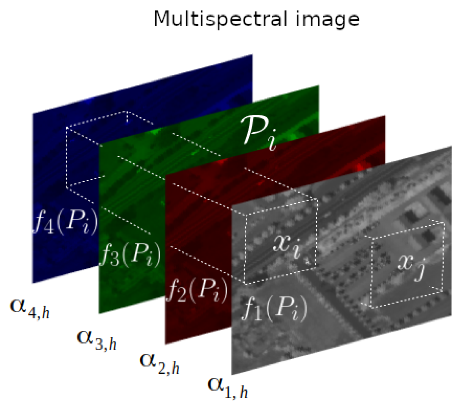
The similarity is computed by considering a 3D volume in the spectral domain centered at each pixel as illustrated in Figure 1. We first compute the Euclidean distance between the 2D patches on each MS band and then average the values linearly using the spectral response S. This would attribute to each band in the MS image its corresponding important in the HS one. The used spectral response S can be represented as the following $M\times H$ matrix:

$$S=\left(\begin{array}{ccccc}{s}_{11}& s_{12}& s_{13}& \cdots & s_{1H}\\ s_{21}& s_{22}& s_{23}& \cdots & s_{2H}\\ ⋮& ⋮& ⋮& ⋮& ⋮\\ s_{M1}& s_{M2}& s_{M3}& \cdots & s_{MH}\end{array}\right).$$

(7)

To some extent, the spectral response is used to interpolate the weights from M to H spectral bands, since they are computed on the MS image but finally differ for each HS band. While other strategies may also be appropriate, the spectral response is suitable because it is used to generate the MS data from the underlying high-resolution HS image.

Let ${\mathcal{P}}_i$ be a 3D volume centered at pixel $x_i$ and extending along the MS dimension. For each $m\in \{1,\dots ,M\}$, let $f_m\left(P_i\right)$ denote the 2D patch obtained as the projection of ${\mathcal{P}}_i$ onto the mth band, so that ${\mathcal{P}}_i$ has M times more pixels than $f_m\left(P_i\right)$. We assume that the radius of each patch $f_m\left(P_i\right)$ is ${\nu }_p\in {\mathbb{Z}}^{+}$. In order to reduce the computational time, the nonlocal operators are calculated in a restricted pixel neighbourhood. Therefore, a search window of radius ${\nu }_{\mathrm{nl}}\in {\mathbb{Z}}^{+}$ is considered at each pixel. In the end, we define the weights as in (8a), where the norms over pixel positions apply by considering the coordinates of each $x_i$ in the Cartesian grid before rasterization, ${\mathsf{\Gamma }}_i$ in (8b) is the normalization factor, and $h_{\mathrm{spt}},h_{\mathrm{sim}}>0$ act like filtering parameters that quantify the speed of decrease of the weights whenever the dissimilarity between the patches becomes important. The weight of the reference pixel with respect to itself is quite important, thus, ${\omega }_{h,i,i}$ is set to the maximum of the weights as given in (8c) in order to avoid excessive weighting. The weight distribution is in general sparse given that only a few nonzero weights are considered in a restricted pixel neighbourhood, thus the space $\mathcal{Y}$ is redefined to be ${\mathbb{R}}^{H\times N\times N_{\mathrm{nl}}}$ with $N_{\mathrm{nl}}={(2{\nu }_{\mathrm{nl}}+1)}^2\ll N$.

$${\omega }_{h,i,j}=\left\{\begin{array}{cc}{\displaystyle \frac{1}{{\mathsf{\Gamma }}_i}}exp\left(-{\displaystyle \frac{\parallel x_i-x_j{\parallel }_2^2}{h_{\mathrm{spt}}^2}}-{\displaystyle \frac{{\sum }_{m=1}^M{s}_{mh}{∥f_m\left(P_i\right)-f_m\left(P_j\right)∥}_2^2}{h_{\mathrm{sim}}^2{(2{\nu }_p+1)}^2{\sum }_{m=1}^M{s}_{mh}}}\right)\hfill & \mathrm{if}{\parallel x_i-x_j\parallel }_{\infty }\le {\nu }_{\mathrm{nl}}\hfill \\ 0\hfill & \mathrm{otherwise}\hfill \end{array}\right.$$

(8a)

$${\mathsf{\Gamma }}_i=\sum _{\{x_j:\parallel x_i-x_j{\parallel }_{\infty }\le {\nu }_{\mathrm{nl}}\}}exp\left(-{\displaystyle \frac{\parallel x_i-x_j{\parallel }_2^2}{h_{\mathrm{spt}}^2}}-{\displaystyle \frac{{\sum }_{m=1}^M{s}_{mh}{∥f_m\left(P_i\right)-f_m\left(P_j\right)∥}_2^2}{h_{\mathrm{sim}}^2{(2{\nu }_p+1)}^2{\sum }_{m=1}^M{s}_{mh}}}\right)$$

(8b)

$${\omega }_{h,i,i}=max\left\{{\omega }_{h,i,j}:{\parallel x_i-x_j\parallel }_{\infty }\le {\nu }_{\mathrm{nl}}\mathrm{and}{x}_j\ne x_i\right\}$$

(8c)

We have adopted a linear variant of the nonlocal regularization since the weights are kept constant along minimization. Similar formulations have been used for deblurring [47], segmentation [48] or super-resolution [49]. There are some inverse problems, such as inpainting [49] and compressive sensing [50], for which getting an accurate estimation of the weights is not feasible. In these scenarios, the regularization is non-linearly dependent on the image to be found, thus, it is necessary to update the weights at each iteration. This makes it hard to get a direct solution and also increases the computational complexity. In our case, given that the MS image provides a good estimation of the weights, a linear nonlocal formulation is more appropriate and also allows an efficient minimization scheme (see Section 3.4).

3.3. Radiometric Constraint

In order to preserve the geometry of the captured scene, we introduce a radiometric constraint that injects the high frequencies of the MS data into the desired fused image. This is based on a similar idea proposed in [18]. In Section 4, we experimentally show that this term allows recovering geometry, texture and fine details so it cannot be omitted in the proposed model.

Let us introduce some notations. We define $P\in \mathcal{X}$ as a linear combination of the MS bands weighted by the entries of the spectral response (7), that is,

$$P_h=\sum _{m=1}^M{\displaystyle \frac{s_{mh}}{s_h}}{f}_m,\forall h\in \{1,\dots ,H\},$$

(9)

where $s_h={\sum }_{m=1}^M{s}_{mh}$. Let $\tilde{g}\in \mathcal{X}$ be the low-resolution HS image upsampled to the high-resolution domain by bicubic interpolation. We apply the spatial degradation in (1) to f and obtain a low-resolution image which is then upsampled by bicubic interpolation, denoted by $\tilde{f}\in \mathcal{X}$. Therefore, $\tilde{f}$ and $\tilde{g}$ contain the low frequencies of the MS and HS data, respectively, and have the same spatial resolutions. We then compute $\tilde{P}\in \mathcal{X}$ as in (9) but using the spectral bands of the interpolated image $\tilde{f}$, that is,

$${\tilde{P}}_h=\sum _{m=1}^M\frac{s_{mh}}{s_h}{\tilde{f}}_m,\forall h\in \{1,\dots ,H\}.$$

We finally impose the radiometric constraint

$${\displaystyle \frac{u_h}{P_h}}={\displaystyle \frac{{\tilde{g}}_h}{{\tilde{P}}_h}},\forall h\in \{1,\dots ,H\},$$

(10)

the variational formulation of which corresponds to the last energy term in (2). The radiometric constraint (10) can be rewritten as

$$u_h-{\tilde{g}}_h=\frac{{\tilde{g}}_h}{{\tilde{P}}_h}\left(P_h-{\tilde{P}}_h\right),\forall h\in \{1,\dots ,H\}.$$

Therefore, we are forcing the high frequencies of each HS band of the fused image, given by $u_h-{\tilde{g}}_h$, to coincide with those of the MS image, given by $P_h-{\tilde{P}}_h$. Consequently, the spatial details of the MS image are injected into the fused product. The modulation coefficient $\frac{{\tilde{g}}_h}{{\tilde{P}}_h}$ can be different for each band and it takes into account the energy levels of the MS and HS data.

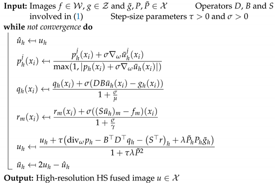
3.4. Saddle-Point Formulation and Primal-Dual Algorithm

The minimization problem (2) is convex but non smooth. In order to find a fast and a global optimal solution we use the first-order primal-dual algorithm introduced by Chambolle and Pock in [51] (CP algorithm). We refer to [52] for all details on convex analysis omitted in this subsection.

On the one hand, any proper, convex and lower semicontinuous function coincides with its second convex conjugate, thus, given that the convex conjugate of a norm is the indicator function of the unit dual norm ball, the dual formulation of (5) is

$${\parallel {\nabla }_{\omega }u\parallel }_1=\underset{p\in \mathcal{Y}}{max}\sum _{h=1}^H\left(\langle {\nabla }_{\omega }{u}_h,p_h\rangle -{\delta }_{{\mathcal{K}}_h}\left(p_h\right)\right),$$

where ${\mathcal{K}}_h=\{p_h\in {\mathbb{R}}^{N\times {(2{\nu }_{\mathrm{nl}}+1)}^2}:\parallel p_h{\parallel }_{\infty }\le 1\}$, ${\delta }_{{\mathcal{K}}_h}$ is the indicator function of ${\mathcal{K}}_h$, $\parallel p_h{\parallel }_{\infty }={max}_{1\le i\le N}\left|p_h\left(x_i\right)\right|$ and $|·|$ denotes the Euclidean norm as in (6).

On the other hand, the efficiency of the CP algorithm is based on the hypothesis that the proximity operators have closed-form representations or can be efficiently solved. This is the case of the $\lambda$-term in (2), but not of those related to the image generation models. For this reason, we dualize the functional with respect to the $\mu$- and $\gamma$-terms as follows:

$$\frac{\alpha }{2}{\parallel x\parallel }_2^2=\underset{y}{max}\langle x,y\rangle -\frac{1}{2\alpha }{\parallel y\parallel }_2^2.$$

The primal problem (2) can be finally rewritten as the saddle-point formulation

$$\begin{array}{cc}\hfill & \underset{u\in \mathcal{X}}{min}\underset{p\in \mathcal{Y},q\in \mathcal{Z},r\in \mathcal{W}}{max}\sum _{h=1}^H\left(\langle {\nabla }_{\omega }{u}_h,p_h\rangle -{\delta }_{{\mathcal{K}}_h}\left(p_h\right)\right)\hfill \\ \hfill & +{\displaystyle \frac{\lambda }{2}}\sum _{h=1}^H{\parallel {\tilde{P}}_h{u}_h-P_h{\tilde{g}}_h\parallel }_2^2\hfill \\ \hfill & +\sum _{h=1}^H\left(\langle DB{u}_h-g_h,q_h\rangle -{\displaystyle \frac{1}{2\mu }}{\parallel q_h\parallel }_2^2\right)\hfill \\ \hfill & +\sum _{m=1}^M\left(\langle {\left(Su\right)}_m-f_m,r_m\rangle -{\displaystyle \frac{1}{2\gamma }}{\parallel r_m\parallel }_2^2\right),\hfill \end{array}$$

where $u\in \mathcal{X}$ is the primal variable, while $p\in \mathcal{Y}$, $q\in \mathcal{Z}$ and $r\in \mathcal{W}$ are the dual variables related to the nonlocal regularization and the two dualized data-fitting terms, respectively.

The CP algorithm requires the use of the proximity operator, which generalizes the projection onto convex sets and is defined for a proper convex function $\phi$ as

$${\mathrm{prox}}_{ϵ}\phi \left(x\right)=\underset{y}{argmin}\left\{\phi \left(y\right)+\frac{1}{2ϵ}{\parallel x-y\parallel }^2\right\},$$

where $ϵ>0$ is a scaling parameter that controls the speed of the movement with which the proximal operator converges to the minimum of $\phi$. Thus, the proximity operator of

$$\begin{array}{cc}\hfill F^{\ast }(p,q,r)& =\sum _{h=1}^H\left({\delta }_{{\mathcal{K}}_h}\left(p_h\right)+\langle g_h,q_h\rangle +\frac{1}{2\mu }{\parallel q_h\parallel }_2^2\right)\hfill \\ \hfill & +\sum _{m=1}^M\left(\langle f_m,r_m\rangle +\frac{1}{2\gamma }{\parallel r_m\parallel }_2^2\right)\hfill \end{array}$$

with respect to p is an Euclidean projection onto the unit $L^2$ norm at each pixel and for each HS band. The remaining proximity operators of $F^{\ast }$ and that of

$$G\left(u\right)=\frac{\lambda }{2}\sum _{h=1}^H{\parallel {\tilde{P}}_h{u}_h-P_h{\tilde{g}}_h\parallel }_2^2$$

have easily computable closed-form expressions. Therefore, the primal-dual scheme for the proposed variational fusion model is given in Algorithm 1. It consists in an ascent step in the dual variables and a descent step in the primal variable followed by over-relaxation.

Algorithm 1: Primal-dual algorithm for minimizing the variational fusion model (2)

4. Method Analysis and Discussion

In this section, we analyze the contribution of the radiometric constraint to the final fused product, study the robustness of the proposed method to noise and aliasing, and discuss on the parameter selection.

For these experiments, we use Bookshelves from Harvard dataset [3] acquired by an HS camera that captures 31 spectral bands and Washington DC which is a remote sensing data [53] with 93 spectral bands. Since the ground truth images are available, we evaluate the results in terms of the root mean squared error (RMSE), which accounts for spatial distortions, and the spectral angle mapper (SAM), which measures the spectral quality.

The reference images are denoised with a routine provided by Naoto Yokoya (https://openremotesensing.net/knowledgebase/hyperspectral-and-multispectral-data-fusion/, accessed on 7 March 2021) [6] before data generation. We simulate the low-resolution HS images by Gaussian convolution of standard deviation ${\sigma }_{\mathrm{blur}}=2$ (unless otherwise stated) followed by downsampling of factor $l=4$. 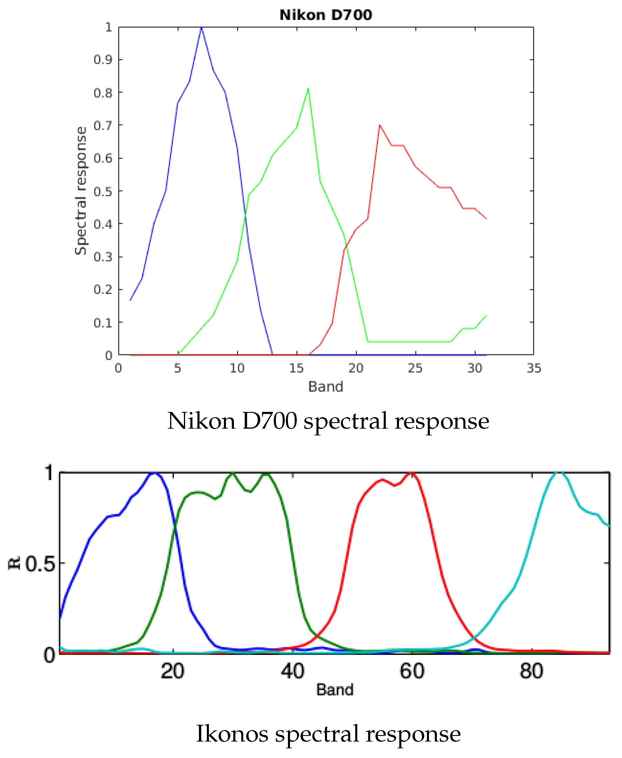The downsampling procedure consists in taking every lth pixel in each direction. The high-resolution MS images are obtained by considering the spectral degradation operator in (7) to be the Nikon D700 spectral response for all experiments on Bookshelves and the Ikonos spectral response on Washington DC (see Figure 2). Unless otherwise stated, we add white Gaussian noise to both HS and MS images in order to have a SNR of 45 dB. The trade-off parameters in (2) are optimized in terms of the lowest RMSE for each experiment in this section.

4.1. Analysis of the Radiometric Constraint

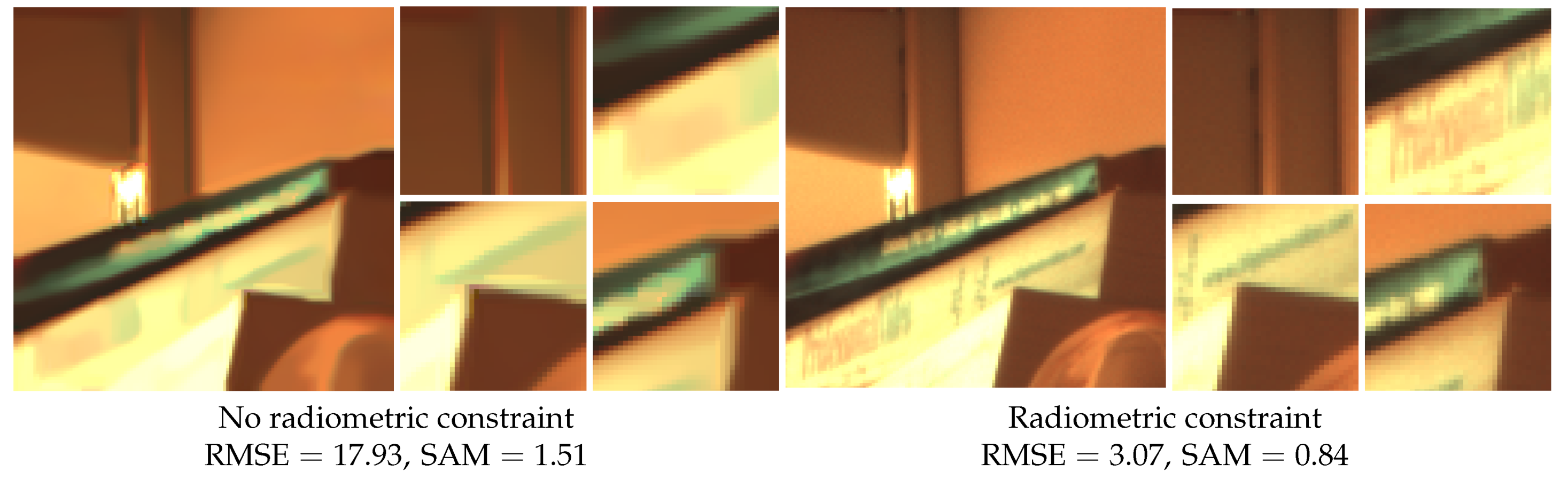
We analyze the contribution of the radiometric contraint (10) to the quality of the final fused product. We use Bookshelves and we launch Algorithm 1 to minimize, on the one hand, the full energy (2) and, on the other hand, the proposed energy without considering the radiometric constraint, which is formally equivalent to set $\lambda =0$ in (2). The respective fused images are shown in Figure 3.

If the radiometric constraint is omitted, spatial details are degraded and not correctly restored, see for instance the contours of the objects and the texts on the book spines. We also notice in this case the appearance of spectral artifacts such as the red spot on the shelf. On the contrary, the fused image obtained when using the full proposed model exhibits better spatial and spectral qualities. Therefore, the radiometric contraint plays an important role in recovering the geometry and the spatial details of the scene and also in avoiding spectral degradations. The numerical results in terms of RMSE and SAM indexes confirm the conclusions drawn visually.

4.2. Robustness to Aliasing in the Low-Resolution Data

Many image acquisition systems suffer from aliasing in the spectral bands that usually produces jagged edges, color distortions and stair-step effects. In the case of MS images, the modulation transfer function (MTF) has low values near Nyquist frequency which leads to avoiding undesirable aliasing effects. On the contrary, for HS images, the MTF has high values at Nyquist frequency which results in present aliasing effects in the spectral data as can be noticed in Figure 4.

In this subsection, the robustness of the variational fusion model to aliasing in the low-resolution HS data is analyzed. We use Washington DC and compare the results obtained on HS images generated with different degrees of aliasing induced by taking ${\sigma }_{\mathrm{blur}}\in \{1,1.3,1.5\}$. Figure 4 shows the respective HS images after bicubic interpolation and the fused results provided by the proposed method. Note that for lower values of ${\sigma }_{\mathrm{blur}}$, the initial data is more aliased but less blurred.

It is noticeable in the interpolated images the relationship between the aliasing and the standard deviation of the blurring kernel. Both the quality metrics and the visual inspection show the ability of our fusion technique to remove aliasing artifacts and drooling effects, i.e., the colors of the objects exceeding their contours, while increasing the resolution of the observations. While aliasing effects diminish, the RMSE of the fused images increases from ${\sigma }_{\mathrm{blur}}=1.3$ to ${\sigma }_{\mathrm{blur}}=1.5$ because more spatial details are compromised by the blur. Since the fused images obtained from data with very different degrees of aliasing are pretty similar, we can conclude that the proposed approach is robust to aliasing.

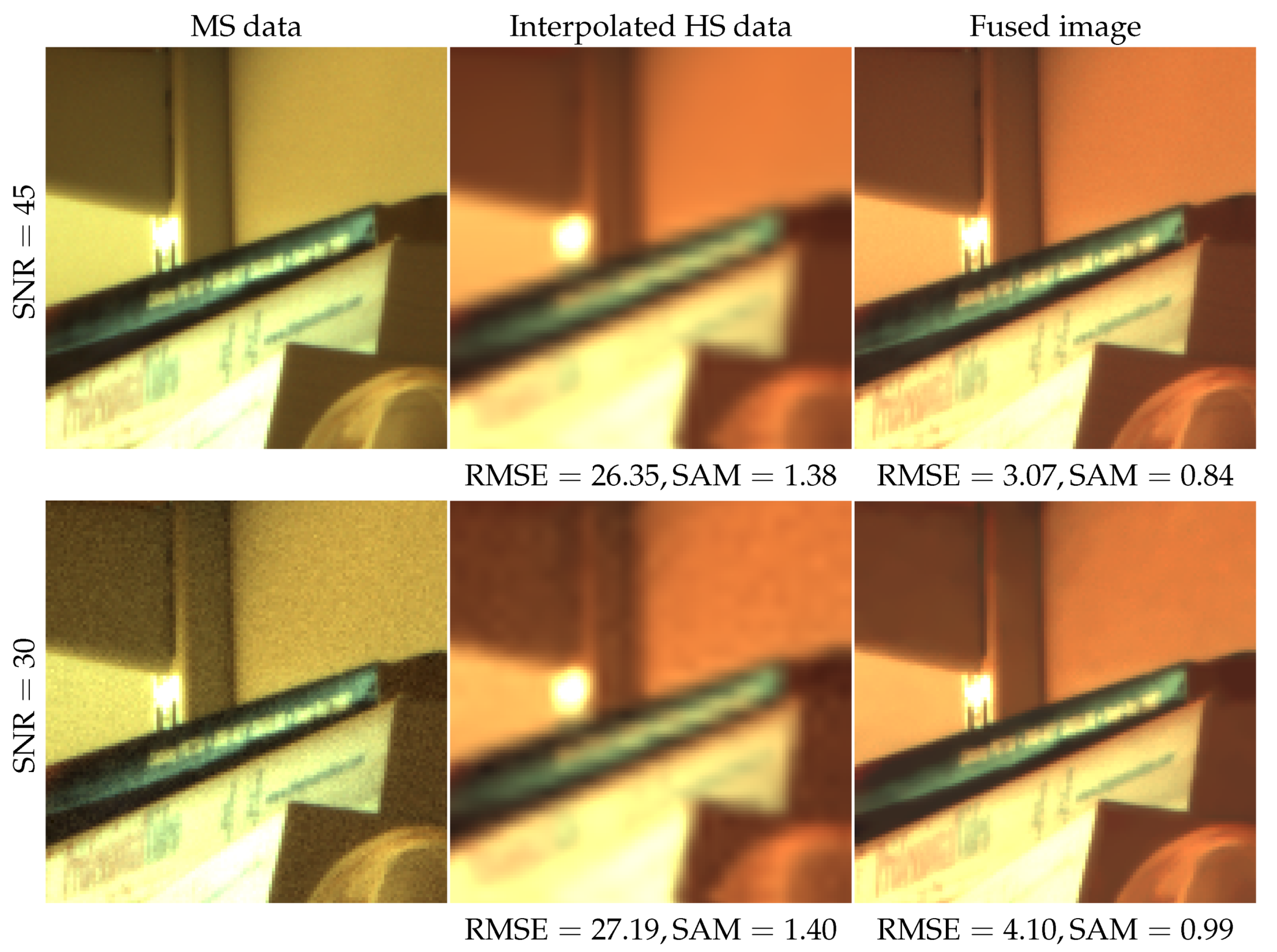
4.3. Robustness to Noise in the Data

We test now the robustness of the proposed fusion method to noise. We use Bookshelves and compare the results obtained by our algorithm on two sets of MS and HS images with different noise levels, $\mathrm{SNR}\in \{30,45\}$ dB. Figure 5 shows the MS images, the HS images after bicubic interpolation and the fused results.

The quality of the interpolated HS images decreases as the noise increases. On the contrary, we correctly deal with different noise levels. Even in the case of low SNR, our algorithm provides a noise-free image and correctly recovers the geometry of the scene. The results for different SNRs looking very similar and yielding almost identical RMSE and SAM values proves the robustness of the method to noise.

4.4. Parameter Selection

The convolution, downsampling and spectral operators used in the energy (2) are the same as those considered for HS and MS data simulation. In our case, we only considered Gaussian convolution kernels since we deal with the aliasing introduced by the relationship between the optics and the sensor size.

For the NL weights in (8), we restrict the nonlocal interactions to a search window of radius ${\nu }_{\mathrm{nl}}=7$, while the radius of the 2D patches considered on each MS band is ${\nu }_p=1$. The filtering parameters are set to $h_{\mathrm{spt}}=2.5$ and $h_{\mathrm{sim}}=10$. The trade-off parameters in the variational formulation (2) have been optimized in terms of the lowest RMSE on Bookshelves for Harvard dataset [3] and on Washington DC [53] for remote sensing data. All experiments have been performed using the same set of parameters.

5. Experimental Results

We evaluate the performance of the proposed variational fusion method and compare with several state-of-the-art and recent techniques on data acquired by commercial HS cameras and Earth observation satellites.

According to the reviews [6,21], we compare with the coupled non-negative matrix factorization unmixing technique [14] (CNMF), the convex variational model with total variation regularization of the subspace coefficients [11] (HySure), the Gram-Schmidt adaptive component-substitution method [6,26] (GSA-HS), the smoothing filtered-based intensity modulation technique [6,27] (SFIM-HS), the generalized Laplacian pyramid approach [6,25] (GLP-HS), the maximum a posteriori estimation with a stochastic mixing model [10] (MAPMM), the Sylvester-equation based Bayesian approach [35] (FUSE), the Wasserstein barycenter optimal transport method [33] (HMWB) and the CNN-FUS method which is based on a convolutional neural network [44]. For HMWB we use the code provided by the authors. Regarding CNN-FUS we use the network weights the authors suggested for any HS and MS image fusion. Finally, for all the other state-of-the-art techniques, we use the codes made available by Naoto Yokoya [6]. In all the experiments, we take the default parameters considered in the corresponding papers.

The availability of the ground truths allows an accurate quality assessment of the fused products. Therefore, we evaluate numerically the results in terms of RMSE and SAM as in the previous section, but also in terms of ERGAS, which measures the global quality of the fused product; $\mathrm{Q}{2}^n$, which evaluates the loss of correlation, luminance and contrast distortions; the cross correlation (CC), which characterizes the geometric distortion; and the degree of distortion (DD) between images. We refer to [6,12,21] for more details on these metrics.

We recall that, the reference images are denoised with a routine provided by Naoto Yokoya [6] before data generation. We simulate the MS and HS data according to the image formation models given in (1). Therefore, the low-resolution HS images are generated by Gaussian convolution of standard deviation ${\sigma }_{\mathrm{blur}}=2$ followed by downsampling of factor $l=4$. The high-resolution MS images are obtained by considering the spectral degradation operator to be the Nikon D700 spectral response on Harvard dataset and the Ikonos spectral response on remote sensing data (see Figure 2). We add white Gaussian noise to HS and MS images in order to have a SNR of 35 dB. From these noisy images, we generate $P_h$, ${\tilde{P}}_h$ and ${\tilde{g}}_h$ required in our model following the procedure described in Section 3.3.

Let us emphasize that neither pre-processing on the input data, which consists of 5 noisy images, nor post-processing on the obtained fused products are applied in the case of our algorithm. For the state-of-the-art methods that do not tackle noise in their models (GSA-HS, SFIM-HS, GLP-HS, MAPMM and HMWB), a post-procesing denoising step is carried out with the routine provided by Yokoya [6]. The HMWB method considers the images as probability measures and provides results that sum to one. Thus, in order to compare the fusion performances with the ones from HMWB, each fusion result from our method and from the state of the art is normalized by the total number of pixels so that it sums to one.

The experiments for this paper were run on a 2.70 GHz Intel Core i7-7500U Asus computer. The overall time for a fusion result is 1.5 min on average. This time includes the computation of the non-local weight matrix which is computed only once before the fusion process and maintained during the iterative procedure. The optimization scheme solved at each iteration contains complex different backward-forward implementations of the gradient and divergence operators that are time consuming. The computational time can be significantly reduced by harnessing parallel computing and better memory access schemes to speed up the weight computations and other steps necessary for the minimization process.

5.1. Performance Evaluation on Data Acquired by HS Cameras

We test the performance of our method on ten images from Harvard dataset [3], representing different indoor and outdoor scenes. These data were acquired by an HS commercial camera (Nuance FX, CRI Inc., Santa Maria, CA, USA)) that captures 31 narrow spectral bands with wavelengths ranging from $420$nm to $720$nm with a step of $10$nm. Each image has a resolution of $1392\times 1040$ pixels, but we cropped them to $512\times 512$ pixels. The reference images are displayed in Figure 6, where 5th, 10th and 25th bands are used to account for the blue, green and red channels. Since Nikon D700 spectral response is used, MS images with three spectral bands are generated.

Table 1. Average of the quality measures over all images of Figure 6, computed after removing a boundary of 5 pixels. RMSE and DD values are expressed in magnitude of ${10}^{-9}$. Best results are displayed in bold and the second best ones are underlined. The proposed method outperforms all other techniques with respect to all evaluation metrics.

	RMSE	SAM	ERGAS	CC	DD	Q2${}^{\mathit{n}}$
Reference	0	0	0	1	0	1
CNMF	10.4862	1.7887	2.3019	0.9917	5.5729	0.9353
HySure	8.0721	2.2296	2.1924	0.9925	5.0001	0.9329
GSA-HS	9.7863	2.3961	2.1880	0.9924	5.6908	0.9327
SFIM-HS	22.0725	1.7659	4.4102	0.9706	10.6725	0.8843
GLP-HS	20.3945	1.9569	4.0528	0.9751	10.6240	0.8921
MAPMM	24.7269	2.2269	4.9971	0.9599	12.2679	0.8530
FUSE	12.0888	1.9744	2.5190	0.9897	6.4420	0.9317
HMWB	8.1404	2.1985	2.8053	0.9835	4.7099	0.9060
CNN-FUS	7.9423	2.9849	2.3130	0.99151	4.929	0.9245
Ours	5.8112	1.6030	1.5313	0.9953	3.7399	0.9376

shows the average of the quality measures over all images of the Harvard dataset (Figure 6) after removing boundaries of 5 pixels. We note that the RMSE and DD values are in magnitude of ${10}^{-9}$. The best results are in bold and the second best ones are underlined. In view of RMSE and ERGAS values, SFIM-HS, GLP-HS and MAPMM are the less competitive in terms of spatial quality. These methods also introduce the largest degrees of distortion (DD) in the fused products. HySure, GSA-HS and CNN-FUS are more affected by spectral degradations as the SAM values point out. Regarding CNMF and FUSE, they seem to have good performance in terms of SAM with relatively high RMSE and DD values. Finally, HMWB has good performance is terms of spectral distortion as shown by the DD measure but performs poorly in ERGAS and Q$2^n$. The proposed fusion approach outperforms all the methods in terms of all numerical indexes.

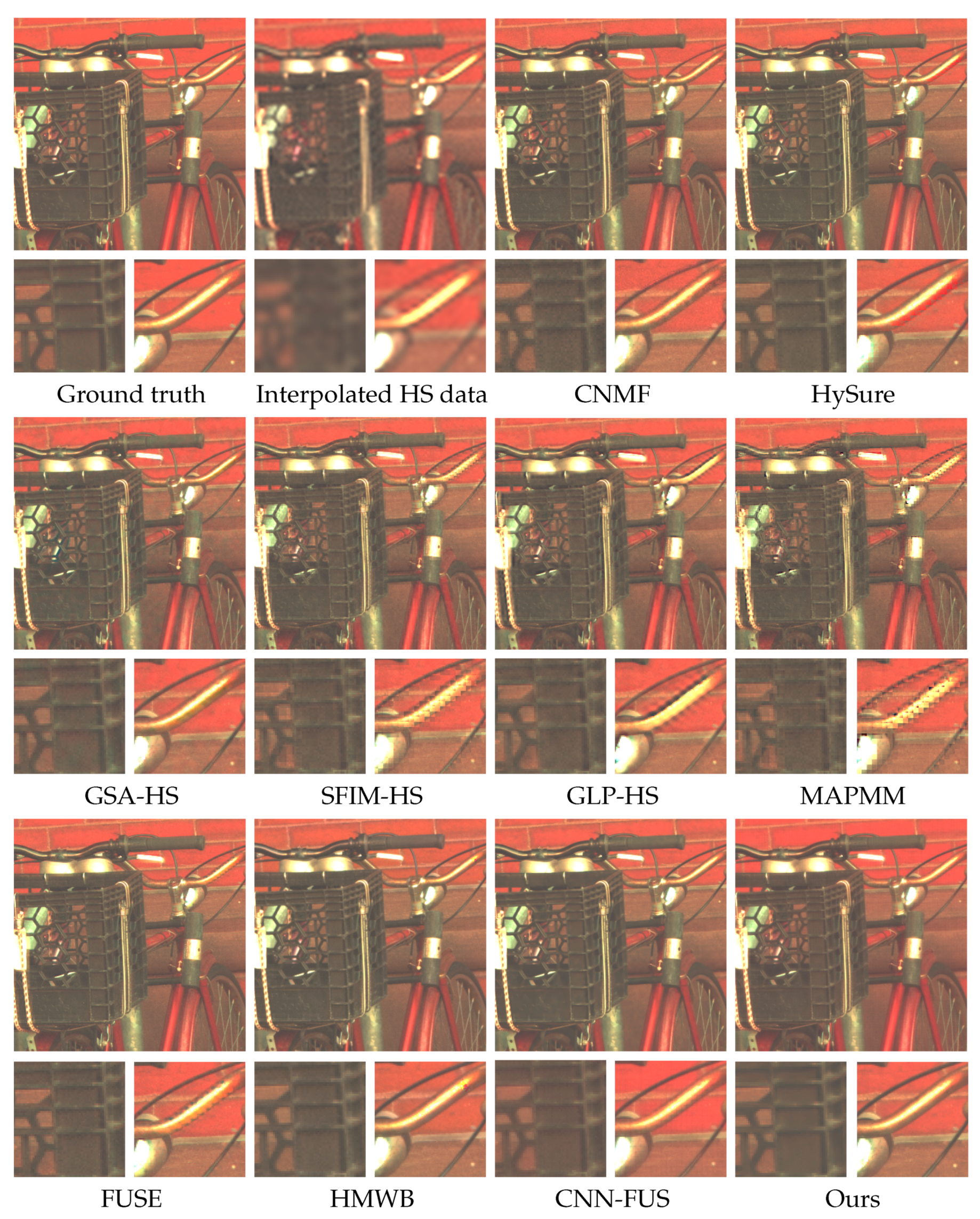
Figure 7 displays the fused images obtained by each technique on Bicycle. As can be noticed on the baskets, all results except the one from CNN-FUS, which is based on a CNN denoiser and ours are noisy. Unlike CNMF, CNN-FUS and our approach, the other methods are also affected by aliasing in the form of color spots and jagged edges, see the metal handlebars. Furthermore, HySure, SFIM-HS, GLP-HS, MAPMM and FUSE have problems at saturated areas such as the reflection on the headlight of the bike. Regarding HMWB and GSA-HS, they suffer from color spots on the metal handlebar and in other parts of the image. We also note that CNN-FUS suffers from repetitive squares that are visible on the handlbars and faint red pixels on the magnified part of the black box. The proposed fusion model successfully combines the geometry contained in the MS image with the spectral information of the HS image, while removing noise and aliasing effects.

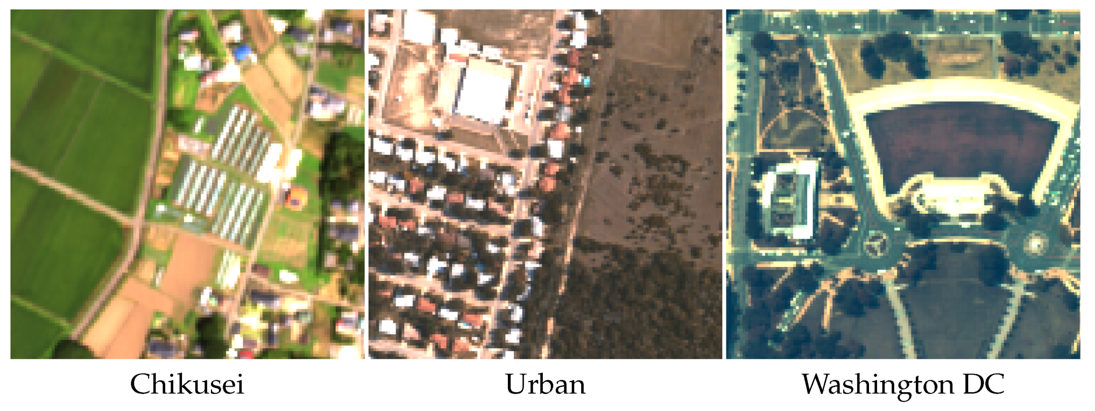
5.2. Performance Evaluation on Remote Sensing Data

In this subsection, we exhibit how fusion techniques behave on remote sensing data. In addition to Washington DC [53], we use Chikusei [54], acquired by the Headwall Hyperspec-VNIR-C imaging sensor with a GSD of $2.5$ m and 128 spectral bands, and Urban (https://www.erdc.usace.army.mil/Media/Fact-Sheets/Fact-Sheet-Article-View/Article/610433/hypercube/, accessed on 7 March 2021), acquired by the HYDICE imaging sensor with a GSD of $2$m and 210 spectral bands. We cropped all the images to $128\times 128$ pixels and reduced the spectral bands to 93. The reference images are shown in Figure 8, with 7th, 25th and 40th spectral bands being displayed to account for the blue, green and red channels. Since Ikonos spectral response is used, MS images with four spectral bands are generated.

The average of the quality measures over all the remote sensing images used in the experiments (Figure 8), are provided in

Table 2. Average of the quality measures over all remote sensing images of Figure 8, computed after removing a boundary of 5 pixels. RMSE and DD values are expressed in magnitude of ${10}^{-8}$. Best results are displayed in bold and second best ones are underlined. The proposed method outperforms all other techniques with respect to all metrics, except CNN-FUS for three metrics.

	RMSE	SAM	ERGAS	CC	DD	Q2${}^{\mathit{n}}$
Reference	0	0	0	1	0	1
CNMF	7.3652	3.2942	3.2900	0.9750	4.8122	0.9577
HySure	6.9567	4.1765	3.4362	0.9748	4.6931	0.9534
GSA-HS	6.7690	3.4157	2.5668	0.9821	4.4959	0.9676
SFIM-HS	10.8585	3.4718	4.5756	0.9440	6.9330	0.9233
GLP-HS	10.2542	3.6230	4.2168	0.9519	5.9117	0.9300
MAPMM	12.5035	4.1206	5.6333	0.9072	7.9438	0.8716
FUSE	9.8776	4.2944	3.9426	0.9550	6.2706	0.9387
HMWB	5.5557	3.1258	2.7468	0.9847	3.1855	0.9675
CNN-FUS	6.1420	3.4497	2.5052	0.9902	4.2926	0.9762
Ours	5.1813	2.8279	2.5589	0.9867	3.1628	0.9718

after removing boundaries of 5 pixels. The RMSE and DD values are expressed in magnitude of ${10}^{-8}$. The best results are displayed in bold and the second best ones are underlined. In the case of satellite data, our method gives the best result in RMSE, SAM and DD and the second best ones in ERGAS, CC and Q$2^n$ after the deep learning based technique CNN-FUS. It is expected that CNN-FUS performs better than our method in some quality metrics given that the used network was trained on multiple satellite images, which makes the fusion performance on satellite data better in some quantitative measures. However, as shown in the previous section, CNN-FUS does not provide the best results on Bicycles. This could be explained by the fact that the CNN-FUS network was not trained on images provided by hyperspectral cameras with a spatial resolution as high as Harvard dataset’s. This shows that deep learning based methods are constrained by the type of data the network was trained on, which limits the performance of the network on unseen data. Nonetheless, our method is more flexible and can be easily applied on any type of images. Regarding the other methods, SFIM-HS, GLP-HS, MAPMM and FUSE perform poorly especially in terms of RMSE and ERGAS. HySure and GSA-HS show good performances in terms of RMSE but high degrees of spectral distortion as shown by the DD index. CNMF and HMWB show competitive performances in terms of SAM with low values in Q$2^n$.

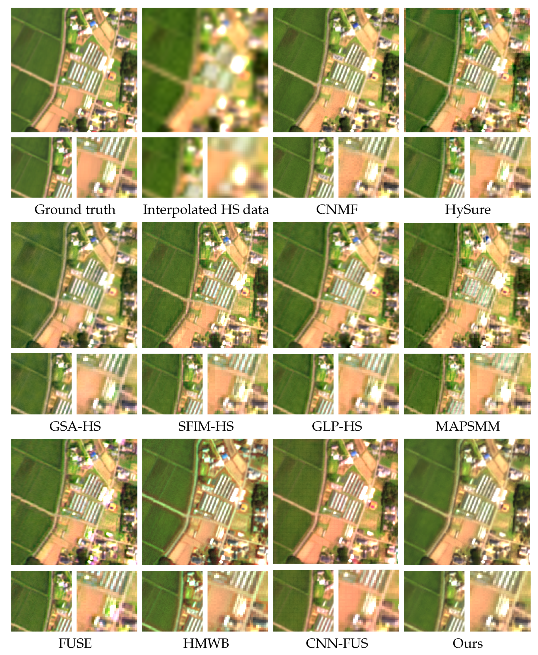
Figure 9 shows a visual comparison of the fused images for Chikusei. All state-of-the-art methods except CNN-FUS are not robust to noise. The proposed approach however is able to remove the noise while preserving the spatial details of the scene. Annoying artifacts further compromise the results provided by HySure, SFIM-HS, MAPMM and FUSE. We also observe that HMWB is not able to correctly recover the spectral information from the HS data, while GLP-HS has problems at saturated areas such as light reflections on the roofs. Moreover, GSA-HS and CNMF provide results visually close to ours but being noisy. Finally, although CNN-FUS produced a non-noisy result, some spatial artifacts are visible such as the repetitive small squares especially in the green parts, highlighted in the magnified images, and also the presence of pink colors on white buildings and elsewhere on the image.

6. Conclusions

We have presented a convex variational model for HS and MS data fusion based on the image formation models. According to these models, the low-resolution HS image is generated by low-pass filtering in the spatial domain followed by subsampling, while the high-resolution MS image is obtained by sampling in the spectral domain taking into account the spectral response function of each band of the MS instrument. The proposed energy functional incorporates a nonlocal regularization term that settles non-linear filtering conditioned to the geometry of the MS image. Furthermore, a radiometric constraint that incorporates modulated high frequencies from MS data into the fused product has been included. In order to compute the solution of the variational model, the saddle-point formulation of the energy has been presented and a primal-dual algorithm has been used for the optimization of the functional.

The analysis of the method has revealed that the radiometric constraint plays an important role in recovering the geometry and the spatial details of the scene and also in avoiding spectral degradation. Furthermore, we have experimentally proven the robustness of our approach to noise and aliasing even though the input data to our model, namely the multispectral, the hyperspectral and the three generated images were all affected by noise. An exhaustive performance comparison, with several classical state-of-the-art fusion techniques and a recent deep learning based one, was carried out. The qualitative measures on data acquired by commercial hyperspectral cameras showed the superiority of our method in all the indexes. Regarding the performances on remote sensing data, only the deep learning based method provides slightly better results in some of the quality metrics, but their fused images are affected by artifacts, which does not happen with the proposed model. Finally, unlike deep learning based techniques, our method can be easily adapted to various types of images from different sensors without any prior knowledge on the data.