Abstract
A single-server non-pre-emptive priority queueing system of a finite capacity with many types of customers is analyzed. Inter-arrival times can be correlated and batch arrivals are allowed. Possible unreliability of the server, implying the loss of a customer or the necessity of its service from the early beginning or some phase of the service, is taken into account. Initial priorities provided to various types of customers at the arrival moment can be varied (increased or decreased) after the random amount of time during the customer stay in the buffer. Such a type of queues arises in the modeling operation of various emergency care systems, information, and perishable goods delivering systems, etc. The stationary behavior of the system is described by the finite state multi-dimensional continuous-time Markov chain with the upper-Hessenberg block structure of the generator. The stationary distribution of the system states and some important characteristics of the system are calculated. The presented numerical examples illustrate opportunities to quantitatively evaluate the impact of the buffer capacity and customers’ mean arrival rate on the most important characteristics of the system. The possibility of solving optimization problems is briefly shown.
1. Introduction
Queueing theory provides a powerful tool for design, capacity planning, performance evaluation, and optimization of many real-world systems. In the simplest settings, all customers of a queueing system are assumed to be homogeneous, having equal requirements and rights to receive service. However, in many real-world systems, this is not true. Some customers or classes of customers, for certain reasons, are more important for the system and are provided higher priority in access to the servers comparing to other classes. These reasons can be versatile. For example, in information transmission systems, signaling information is much more important than the information sent by the users, time-sensitive information should be transferred earlier than the elastic insensitive information. In intellectual vehicular networks, the transmission of driving safety information is much more urgent than the transmission of the info-entertainment information. Processing of information generated by the certified user is more urgent than the processing of information by the cognitive user in cognitive radio systems. The handover user who arrived at the cell of a mobile network has to be treated differently than the new user trying to establish a connection within a given cell, etc. In emergency service systems, in particular, an emergency healthcare system, the patients can be sorted and treated by injury severity. In food delivery services, the most rapidly deteriorating (perishable) items have to be delivered first. In communication systems, the clients can sign agreements with different service levels (and different fees). The ultra-reliable low-latency communication (URLLC) applications in 5G networks have higher priority than the enhanced mobile broadband (eMBB) applications, etc. A proper choice of the priorities can significantly increase the economic profit gained from the operation of a corresponding system and revenue generating businesses. Therefore, the priority queueing models have attracted a lot of attention from researchers. In the overwhelming majority of the existing research, the priorities (non-pre-emptive or pre-emptive) are assigned from the early beginning and remain permanently valid.
However, there exist a lot of various situations where it is necessary to be more flexible and change the current priorities of customers. For example, in an emergency healthcare system, after assigning the priorities to various customers as the result of the initial triage, the state of the health of a patient can become essentially worse during his or her waiting for the treatment and his or her priority has to be increased. In dispatching the ambulance cars, the priority of an initially non-urgent patient can increase due to approaching some existing deadline for the provision of an ambulance. The same situation occurs in signal processing systems with information obsolescence in which the further processing of the signal becomes meaningless after some amount of time.
The short surveys of the literature devoted to the queueing systems with changing the priority of customers are given, e.g., in [1,2,3,4,5,6,7,8,9,10,11]. In [5,6,7,8], the change of the priority occurs deterministically as a function of the elapsed sojourn time. In the rest of the cited papers, the change of the priority occurs stochastically after some random time. In [1], a table giving the brief classification of the existing results for the case of the stochastic change is presented. The existing papers are classified according to the number of priority classes, arrival process, distribution of the service time, and time until the change of the priority and the obtained results. The model considered in paper [1] is the most general with respect to the pattern of the arrival process and the distribution of the service time and time until the change of the priority. The main restriction of this paper is that only the case of two priority classes is dealt with. The closest queueing system to the model considered in this paper was analyzed in paper [12]. That queueing system has a single-server and a buffer of a finite capacity. Arriving customers are heterogeneous and impatient. Impatience depends on the type of a customer. Different types of customers are assigned the different non-pre-emptive priorities at an arrival moment. However, after the exponentially distributed interval of time during the stay in the buffer, the established priority of a customer can increase. This can occur several times during the customer waiting time. The dynamics of the considered system is described in [12] by the multi-dimensional continuous-time Markov chain. The generator of this chain is obtained, the problem of computation of the stationary state probabilities is touched. Explicit formulas for computing the key performance measures of the system via the obtained stationary probabilities are derived. The dependencies of certain performance measures on the capacity of the buffer are graphically illustrated. The importance of account of correlation in the arrival process and variance of the service time is numerically confirmed.
The distinguishing features of the model considered in this paper comparing to [12] are the following ones:
- The batch arrival of customers of different classes in the batch marked Markov arrival process (BMMAP), which is typical in many real-world systems, is supposed while the customers arrive only one-by-one in the marked Markov arrival process (MMAP) in [12];
- The server is supposed to be unreliable with the options of the loss of a customer, during service of which the breakdown occurs, service repetition from the beginning or from the phase of service at which the breakdown occurs, while the server is assumed reliable in [12];
- Both possibilities of the priority increase and decrease are explored here while only the case of the possible increase of the priority is supposed in [12].
The brief outline of the paper is as follows. In Section 2, the mathematical model is described. In Section 3, the operation of the system is described by the multi-dimensional continuous-time Markov chain with the upper-Hessenberg block structure of the generator. Some results from [12] and their extensions are used to compute the blocks of the generator. A numerically stable algorithm for computation of the stationary distribution of this Markov chain, which essentially exploits the revealed structure of the generator, is presented. Formulas for computation of the key performance measures of the system based on the knowledge of the stationary distribution of the Markov chain are presented in Section 4. Section 5 contains the numerical results that show the dependencies of some performance measures (including the average number of customers of different types in the buffer and customer loss probabilities due to the buffer overflow, breakdown of the server, and impatience of the customers) on the buffer capacity and the average arrival rate. The possibility of the optimal choice of the capacity of the buffer, which guarantees that the loss probability does not exceed the pre-assigned small value, is illustrated. It is numerically shown that sometimes, due to the existence of customer losses caused not by the buffer overflow but by the server unreliability or customers impatience, it is not possible to decrease the loss probability to some admissible level by means of the corresponding increase of the buffer capacity. Section 6 concludes the paper.
2. Mathematical Model
We consider a single-server queueing system with a finite buffer of capacity N and R types of customers. The structure of the system is presented in Figure 1.
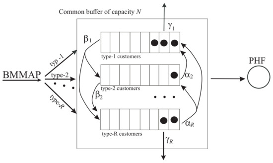
Figure 1.
Structure of the system.
Customers of different types have identical requirements to the service process but different priorities. We assume that the types of customers are enumerated in the decreasing order of the priority. This means that type-1 customers have the highest priority, etc., type-R customers have the lowest priority. We assume that a customer having the highest priority among the presented in the buffer is selected for service at any service completion epoch.
The input flow of customers is described by the . Customers arrival in the is defined by the irreducible continuous time Markov chain , having the finite state space . The sojourn time of the chain , in the state is exponentially distributed with a positive parameter . After this time expires, with probability this chain jumps into the state without generation of customers and with probability the chain jumps into the state and a batch consisting of k customers of type-r is generated. Here, we assume that the maximal batch size of type r customers is limited by the parameter . Let us denote as K the maximal batch size among all types of customers, i.e.,
The parameters defining the can be stored in the square matrices of size W defined by their entries:
The matrix
is a generator of the Markov chain
Let us denote as the stationary probability vector of the states of the Markov chain
This vector can be found as the unique solution to the system
Hereinafter, is a zero row vector and is the column vector consisting of ones.
The average intensity of type-r customers arrival is defined as
The average intensity of batches of type-r customers arrival is calculated by
The average intensity of customers arrival is defined as
For more information about the , see, e.g., [13].
If a batch of customers of any type arrives when the server is idle, the first customer of the batch immediately starts processing by the server (service), and the rest of the customers are placed into the buffer. If the capacity of the buffer is not enough for storing all the customers from the batch, the customers, for which there is not enough buffer space, leave the system permanently (are lost). This means that we assume the partial admission discipline.
During the stay in the buffer, each customer of type- can change (increase or decrease) its priority. Obviously, for most applications, it is sufficient to consider the model with increasing priority of customers. However, for the mathematical generality of the model and having in mind the potential application in information processing systems where long waiting implies the obsolescence of information and the decrease of its value, we consider the possibility of both increasing and decreasing the priority. We assume that after an exponentially distributed time with the parameter any type- customer becomes a type-l customer with the probability independently of other customers. Here, After the exponentially distributed time with the parameter any type-r customer becomes a type-l customer with the probability independently of other customers. Here,
Customers can be impatient and leave the buffer without service, independently of other customers. If, during an exponentially distributed with parameter time, a type-r customer does not succeed to enter the service, this customer departs from the system permanently (is lost), If, during the stay in the buffer, the customer changes his or her priority and becomes type- customer, the patience time restarts and has an exponential distribution with the parameter We denote
Customers’ service times have the so called phase-type distribution with failures (), see [14]. This distribution is an essential generalization of the classical phase-type distribution. The duration of a service time and the result of service are defined by the continuous-time underlying Markov chain having a finite state space Here, the states are transient while the states and are the absorbing states. The initial state of the underlying Markov chain at the service beginning moment is randomly chosen from the set of the transient states. The probabilities defining the choice are given by the components of the stochastic row vector The intensities of the transition between transient states (phases) of the process are defined by the entries of the sub-generator
The transition of the chain to one of the two absorbing states corresponds to the end of the current stage of the service. The transition intensities of the chain to the absorbing state are given by the components of the column vector The transitions to the absorbing state correspond to the successful service of a customer. The intensities of the transition to this state are given by the components of the column vector The transition of the chain to the absorbing state means the end of the stage of the service due to a failure occurrence. When a failure occurs, then the serviced customer is lost with probability restarts service from the early beginning with probability and continues service from the phase at which the failure occurred with probability
For more information about distribution and its properties see [14,15].
3. Process of the System States
The behavior of the system under study can be described by the regular irreducible continuous-time Markov chain
where, during the epoch
- is the number of customers in the system,
- is the state of the underlying process of the ,
- is the state of the underlying process of service process,
- is the number of type-r customers in the buffer, ,
To investigate the Markov chain let us enumerate its states in the direct lexicographic order of the components and , and the reverse lexicographic order of the components
Let us firstly consider the process Under the fixed total number n of customers in the buffer, the components of the R-dimensional process describe the dynamics of the number of customers of different types currently presenting in the buffer. To describe transition intensities of this process, we use several auxiliary matrices.
- (a)
- The intensities of transition of this process when some customer departs from the buffer due to impatience are the elements of the matrix
- (b)
- The intensities of transition of this process when some customer changes the priority are the elements of the matrix Here, the matrix H defines the intensities of increasing and decreasing of priorities. It is described by formula:
- (c)
- The transition probabilities of the process when a new customer arrives and is admitted to the system are the elements of the matrix Here, the entries of the row vector are the probabilities that the arrived to the system customer has type-
- (d)
- The transition probabilities of the process when new customer is picked up for service are the elements of the matrix This customer has the highest priority among all customers currently waiting in the system.
The algorithms for computation of the matrices and and their proofs are presented in [12].
Let us introduce the following notation:
- ⊗ and ⊕ indicate the symbols of the Kronecker product and sum of matrices, respectively, see [16];
- where is the diagonal matrix with the diagonal elements listed in the brackets;
By analyzing all possible transitions of the Markov chain during an interval of infinitesimal length and rewriting the intensities of these transitions in the block matrix form, we obtain the following result.
Theorem 1.
The infinitesimal generator Q of the Markov chain has the following block-tridiagonal structure
The non-zero blocks are defined as follows:
where
where
Proof.
The proof of the theorem is based on the analysis of all possible transitions of the Markov chain during the time interval of infinitesimally small length. The diagonal entries of the matrices are negative. The moduli of these elements define the total intensity of the exit of the Markov chain from the corresponding state.
- In the case the system is empty and the Markov chain can only leave its state when the underlying process of the arrival flow makes a transition from one state to another. The intensities of such transitions are defined by the modulus of the diagonal entries of the matrix
- In the case the server is busy and the buffer is empty. In this case, the Markov chain can leave its current state also due to a transition in the underlying process of service. The intensities of the underlying process of service exit from its states are given as the modulus of the diagonal entries of the matrix S and the total intensities of transitions of the service and arrival process in the case are given as the modulus of the corresponding entries of the matrix . However, not all the transitions of the service process lead to the change of the state of the chain There are possible situations when the service process transits from some state to the second absorbing state, a failure occurs and a customer who received service when a failure occurred, restarts the service from the same state. When such a situation occurs, the chain does not exit from its state. The intensities of such transitions are given by the diagonal entries of the matrix Thus, the total intensities of the leaving the states of the Markov chain in the case are given by the modulus of the corresponding entries of the matrix defined by formula (1);
- In the case there are customers in the buffer. Therefore, in contrast to the case the Markov chain can also leave its state due to a transition of the process that describes the dynamics of the types of the customers staying in the buffer. The intensities of transitions of the process are given as the modulus of the diagonal entries of the matrix . Thus, the total intensities of the leaving the states of the Markov chain in the case are given by the modulus of the corresponding entries of matrix (2);
- In the case the Markov chain can leave its state due to the same reasons as in the previous case. The reason why we separately consider this case is the following. When the buffer is full, the situation is possible when the underlying process of the makes a transition from one state to the same state with the generation of a batch of customers (transitions to the same state without a batch generation are not allowed in ). Since the buffer is full, the arriving batch will be lost. So, such a transition does not change the state of the Markov chain and it is required to add to the negative diagonal entries of the matrix the positive diagonal entries of the matrix . Thus, the total intensities of the exit from the states of the Markov chain in the case are given by the modulus of the corresponding entries of matrix (3).
The non-diagonal entries of the matrices are positive and define the intensities of the Markov chain transitions that do not lead to the change the number of customers in the system These transitions are:
- The transitions of the underlying process without generation of a batch (the intensities are defined by non-diagonal entries of the matrix ) in the case
- The transitions of the service process to the second absorbing state which are accompanied with the restart of the service of a customer from the beginning from another state (they are defined by the non-diagonal entries of the matrix ) in the case
- The transitions of the process due to the change of the priority by some customer (the intensities of such transitions are defined by non-diagonal entries of the matrix ) in the case
- The transitions of the underlying process with generation of a batch to the same state (the intensities are defined by non-diagonal entries of the matrix ) in the case
Taking into account all these reasonings, we obtain the form of the diagonal blocks of the generator Q.
The entries of the matrices are positive and define the intensities of the Markov chain transitions that lead to the increase in the number of customers in the system from n to . The entries of the matrix define the intensity of the chain transitions that lead to the increase in the number of customers in the system from 0 to 1. Such transitions occur when exactly one customer of any type arrives at the empty system. In this case, we have to establish the state of the service process according to the probabilistic vector Thus, the matrix has form (4).
The entries of the matrices define the intensity of the chain transitions that lead to the increase in the number of customers in the system from 0 to n. Such transitions occur when exactly n customers of any type arrive at the empty system. In this case, except for the establishing the state of the underlying process of service, we also have to establish the states of the process that describes the transitions of the number of different types of customers in the buffer using the matrices , in the case of type-r customers arrival. Note, the arrival of n type-r customers is not possible when n is greater than the maximal batch size For accounting such situations we introduce the matrices . Thus, the matrices have form (5).
The matrix is not zero only when The entries of this matrix give the transitions of the chain that lead to the arrival of more than N customers to the empty system. The explanation of form (6) of the matrix is the same as in the previous case. The form of the matrices and can be explained similarly as above, only taking into account that there is no need to establish the state of the service process because the server is busy in these cases. Taking into account all these reasonings we obtain the form of the blocks of the generator Q.
The entries of the matrices are positive and define the intensities of the Markov chain transitions that lead to the decrease in the number of customers in the system by one. In the case such a decrease occurs when the service of a customer is successfully finished or terminated due to a failure occurrence with subsequent loss of the customer under the service. The intensities of such transitions are given by the entries of the matrix In the case such a decrease also can occur due to the successful service or loss of a customer due to the failure. Since the buffer is not empty, in such a situation it is necessary to choose a customer with the highest priority from the buffer and establish the state of a new service process. Besides this, such a decrease can occur due to the customer loss from the buffer due to impatience. The intensities of such transitions are given by the matrix Taking into account all these reasonings, we obtain the form of the blocks of the generator Q. Since the customers are serviced only one by one, the service completion of two or more customers during a infinitesimally small time interval is impossible. Thus, are zero matrices. □
The Markov chain has a finite state space and is irreducible. This implies that, the steady-state probabilities of the system
exist for all values of the system parameters.
Let these probabilities be enumerated in the reverse lexicographic order of the components and the direct lexicographic order of the components and into the row vectors of
The vectors satisfy the following system of equilibrium (Chapman-Kolmogorov) equations:
where Q is the infinitesimal generator of the Markov chain .
If the number of equations of system (7) is large, to solve it one should use an algorithm that takes into account the sparse structure of the generator We propose the following Algorithm 1.
The idea of this algorithm is to substitute the system (7) with the system of equilibrium equations for the family of specially constructed censored Markov chain with varying censoring levels for the initial Markov chain This idea is borrowed from the paper [17] where the analyzed Markov chain had an infinite state space. The presented above algorithm is essentially less memory consuming than the algorithm that is the direct adaptation of the algorithm from [17]. The latter algorithm has a step similar to step 3 in the presented algorithm. However, in [17] the sequence of the matrices of size is recursively computed and stored while in the presented algorithm we recursively compute and store only the row vectors of size
| Algorithm 1: Computation of the probability vectors |
|
4. Performance Measures
When the stationary probabilities have been computed, we can find different system performance measures.
The average number of customers in the buffer is
The average number of type- customers in the buffer can be computed as
Here, the matrix is computed by the same formulas as the matrix with replacement of the vector of impatience rates by the stochastic vector
The output rate of successfully serviced customers is
The output rate of customers who leave the system due to service failure is
The output rate of customers who leave the buffer due to impatience is
The probability of loss of an arbitrary customer is computed as
The probability of loss of an arbitrary customer due to service failure is computed as
The probability of loss of an arbitrary customer due to impatience is computed as
The output rate of the type- customers who leave the buffer due to impatience is
where is the row vector of size R with all zero entries except the r-th entry which is equal to
The average rate of changing the types- of a customer to type- is computed as
The average rate of of changing the types- of a customer to the type- is computed as
The probability that an arbitrary type-r customer will be lost due to impatience can be computed
Here, we assume that and
The probability of an arbitrary type-r customer loss upon arrival is
The probability of an arbitrary customer loss upon arrival is
Remark 1.
To control the accuracy of calculations, the following equality can be used
5. Numerical Example
In this numerical experiment, we assume that the number of types of customers is
The matrices and , which define the , are given by
These matrices provide the value of intensities such as The total customers arrival intensity is
We assume that the distribution of the service time is defined by the vectors the matrix and the probabilities
The mean service time (successful or not) is
The intensities and probabilities that define the changes of customers priorities are the following: , The intensities of impatience are
Let us vary the values of the buffer capacity N over the interval with step 1. Also, we vary the values of the total arrival intensity over the interval with step 0.25. It is done using multiplication of the matrices and by the corresponding intensity For example, the with matrices and has the total arrival intensity
Figure 2, Figure 3, Figure 4 and Figure 5 illustrate the dependence of the average number of customer in the buffer and average number of type- customers in the buffer on the buffer capacity N and average total arrival rate
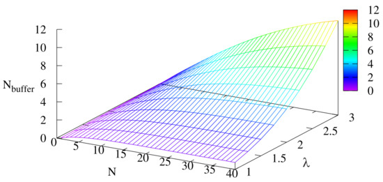
Figure 2.
Dependence of on N and .
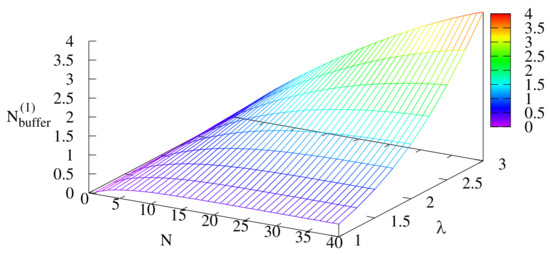
Figure 3.
Dependence of on N and .
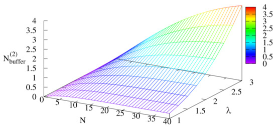
Figure 4.
Dependence of on N and .
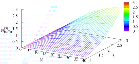
Figure 5.
Dependence of on N and .
As it is seen from Figure 2, Figure 3, Figure 4 and Figure 5, the average numbers of customers (total and of each type) in the buffer increase with the increase of the buffer capacity and the average arrival rate.
Figure 6 illustrates the dependence of the probability of an arbitrary customer loss upon arrival on the buffer capacity N and average total arrival rate
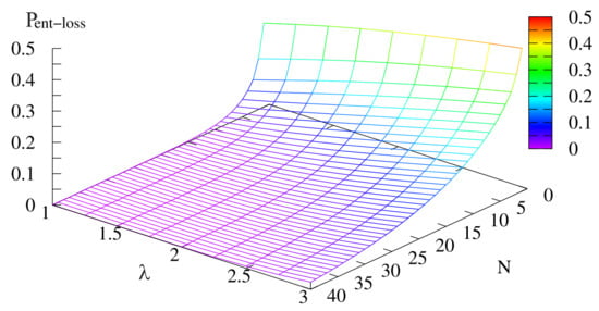
Figure 6.
Dependence of the probability on N and .
The loss probability decreases with the increase of the buffer capacity N and increases with the increase of the arrival intensity . Our results allow us to estimate this intuitively clear dependence quantitatively.
Figure 7 shows the dependence of the probability of loss of an arbitrary customer due to service failure on the buffer capacity N and average total arrival rate
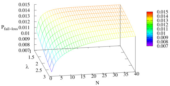
Figure 7.
Dependence of the probability on N and .
The loss probability increases with the increase of the buffer capacity N and decreases with the increase of the arrival intensity . When the buffer capacity N increases and the arrival intensity decreases, the share of customers that succeed to reach the server grows, which implies the increase of the loss probability
Figure 8 illustrates the dependence of the probability of loss of an arbitrary customer due to impatience on the buffer capacity N and average total arrival rate
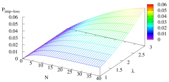
Figure 8.
Dependence of the probability on N and .
The loss probability grows with the increase of the buffer capacity N. It can be explained as follows. With the growth of N, the number of customers staying in the buffer increases, and more customers leave the buffer due to impatience. The behavior of the loss probability with the increase of can be not monotonic. For example, for for the loss probability , for the loss probability , and for the loss probability . This is because the increase of leads, on the one hand, to the increase in the number of customers in the buffer that has to increase the probability but on the other hand, the increase of implies the growth of the share of the customers that leave the system upon arrival and cannot be lost due to impatience.
Figure 9 illustrates the dependence of the loss probability of an arbitrary customer on the buffer capacity N and average total arrival rate
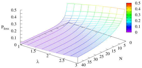
Figure 9.
Dependence of the probability on N and .
As it is seen from Figure 9, the loss probability increases with the increase of the average total arrival rate and the decrease of the buffer capacity
Using the obtained results we can solve various optimization problems. For example, let the optimization problem be formulated as follows: it is required to determine the minimal buffer capacity that guarantees the fulfillment of the inequality
In the considered example, for the average total arrival rate the optimal value of the buffer capacity is and the corresponding loss probability is equal to
For the average total arrival rate the optimal value of the buffer capacity is and the corresponding loss probability is equal to
For the average total arrival rate the optimal value of the buffer capacity is and the corresponding loss probability is equal to
For the average total arrival rate the optimal value of the buffer capacity is and the corresponding loss probability is equal to
For the average total arrival rate the optimal value of the buffer capacity is and the corresponding loss probability is equal to
For the average total arrival rates and 3, it is impossible to determine the optimal buffer size only from the values presented on Figure 9 because for all these arrival intensities. In the case of the optimal solution doesn’t exist because the value of the probability of loss of an arbitrary customer due to impatience when is equal to 0.05445345, and as we mentioned above, this probability grows with the increase of buffer capacity N. So, the loss probability in the case is greater than 0.05445345 for all
In the cases and the probability of loss of a customer due to impatience when is less than 0.05 (0.04119366 and 0.0478299, respectively). However, the sum of probabilities and is 0.05485347 in the case and 0.061301324 in the case and exceeds the value 0.05. Since the loss probability also increases with increase of N, the optimal solution doesn’t exist in the case and
In the case of it is necessary to increase the buffer capacity to obtain the optimal solution. In the considered example, the optimal buffer capacity is , and the corresponding loss probability is equal to
6. Conclusions
A single-server queueing model with a buffer of a finite capacity, heterogeneous correlated arrival process with the possibility of batch arrivals and non-pre-emptive priorities is analyzed. Customers are impatient with the impatience rate depending on the type of the customer. The server is unreliable. The priorities can be changed (increased or decreased) randomly in the Markov manner during the customer’s stay in the buffer. The stationary behavior of the system having the listed features is analyzed via the analysis of the properly constructed Markov chain. The numerical results give some insight into the dependence of the main performance measures of the system on the total arrival rate and capacity of the buffer. The possibility of achieving the admissible value of an arbitrary customer loss probability via the proper choice of the buffer capacity is discussed.
As the directions for further research, generalizations of the model to the cases with a dependence of service time distribution on the type of a customer, possibility of the service pre-emption and the loss of the customers whose service is interrupted or their retrials deserve investigation in the future.
Author Contributions
Conceptualization, S.D. and A.D.; methodology, S.D., O.D., and K.S.; software, S.D. and O.D.; validation, S.D. and O.D.; formal analysis, S.D., K.S., and A.D.; investigation, A.D.; writing, original draft preparation, K.S. and A.D.; writing, review and editing A.D. and K.S.; supervision A.D. and K.S.; project administration O.D. and A.D. All authors read and agreed to the published version of the manuscript.
Funding
The publication was prepared with the support by the RUDN University Strategic Academic Leadership Program.
Institutional Review Board Statement
Not applicable.
Informed Consent Statement
Not applicable.
Data Availability Statement
Not applicable.
Conflicts of Interest
The authors declare no conflict of interest.
References
- Klimenok, V.; Dudin, A.; Dudina, O.; Kochetkova, I. Queuing System with Two Types of Customers and Dynamic Change of a Priority. Mathematics 2020, 8, 824. [Google Scholar] [CrossRef]
- Cao, P.; Xie, J. Optimal control of a multiclass queueing system when customers can change types. Queueing Syst. 2016, 82, 285–313. [Google Scholar] [CrossRef]
- He, Q.-M.; Xie, J.; Zhao, X. Priority Queue with Customer Upgrades. Nav. Res. Logist. 2012, 59, 362–375. [Google Scholar] [CrossRef]
- Xie, J.; Cao, P.; Huang, B.; Ong, M.E.H. Determining the conditions for reverse triage in emergency medical services using queuing theory. Int. J. Prod. Res. 2012, 54, 3347–3364. [Google Scholar] [CrossRef]
- Fajardo, V.A.; Drekic, S. Waiting Time Distributions in the Preemptive Accumulating Priority Queue. Methodol. Comput. Appl. Probab. 2017, 19, 255–284. [Google Scholar] [CrossRef]
- Mojalal, M.; Stanford, D.A.; Caron, R.J. The lower-class waiting time distribution in the delayed accumulating priority queue. INFOR Inf. Syst. Oper. Res. 2020, 58, 60–86. [Google Scholar] [CrossRef]
- Sharma, K.C.; Sharma, G.C. A delay dependent queue without preemption with general linearly increasing priority function. J. Oper. Res. Soc. 1994, 45, 948–953. [Google Scholar] [CrossRef]
- Stanford, D.A.; Taylor, P.; Ziedins, I. Waiting time distributions in the accumulating priority queue. Queueing Syst. 2014, 77, 297–330. [Google Scholar] [CrossRef]
- Xie, O.; He, Q.-M.; Zhao, X. Stability of a priority queueing system with customer transfers. Oper. Res. Lett. 2008, 36, 705–709. [Google Scholar] [CrossRef]
- Xie, J.; Zhu, T.; Chao, A.K.; Wang, S. Performance analysis of service systems with priority upgrades. Ann. Oper. Res. 2017, 253, 683–705. [Google Scholar] [CrossRef]
- Cildoz, M.; Ibarra, A.; Mallor, F. Accumulating priority queues versus pure priority queues for managing patients in emergency departments. Oper. Res. Health Care 2019, 23, 100224. [Google Scholar] [CrossRef]
- Lee, S.K.; Dudin, S.; Dudina, O.; Kim, C.S.; Klimenok, V. A Priority Queue with Many Customer Types, Correlated Arrivals and Changing Priorities. Mathematics 2020, 8, 1292. [Google Scholar] [CrossRef]
- Khalid, A.; Dudin, A.; Mushko, V. Novel queueing model for multimedia over downlink in 3.5 G wireless network. J. Commun. Softw. Syst. 2006, 2, 68–80. [Google Scholar]
- Dudin, A.; Dudin, S. Analysis of a Priority Queue with Phase-Type Service and Failures. Int. J. Stoch. Anal. 2016, 2016, 9152701. [Google Scholar] [CrossRef]
- Dudin, S.; Dudina, O. Retrial multi-server queuing system with PHF service time distribution as a model of a channel with unreliable transmission of information. Appl. Math. Model. 2019, 65, 676–695. [Google Scholar] [CrossRef]
- Graham, A. Kronecker Products and Matrix Calculus with Applications; Horwood, E., Ed.; Courier Dover Publications: Cichester, UK, 1981. [Google Scholar]
- Klimenok, V.I.; Dudin, A.N. Multi-dimensional asymptotically quasi-Toeplitz Markov chains and their application in queueing theory. Queueing Syst. 2006, 54, 245–259. [Google Scholar] [CrossRef]
Publisher’s Note: MDPI stays neutral with regard to jurisdictional claims in published maps and institutional affiliations. |
© 2021 by the authors. Licensee MDPI, Basel, Switzerland. This article is an open access article distributed under the terms and conditions of the Creative Commons Attribution (CC BY) license (https://creativecommons.org/licenses/by/4.0/).