1. Introduction
An involute of a curve in Euclidean plane
is a curve to which all tangent lines of the initial curve at corresponding points are orthogonal. If
is a curve in
parametrized by arc length, then the parametrizations of its involutes are
where
is a constant, and
. It is clear that all involutes for different constants
a are mutually parallel curves. An evolute of a curve
c in
is a curve
e whose involute is the very curve
c, so evolutes and involutes are, in a sense, inverses of each other. Involutes and evolutes of curves in Euclidean plane were introduced already in 1670’s by Huygens in relation to his work with pendular motion and the isochronous pendulum [
1].
When a curve
c parametrized by arc length is given, then its evolute is sought-after in the form
, where
is the unit normal field of
c. The condition that tangent lines of a curve and its evolute are orthogonal which implies
where
is the curvature of
c. So, the evolute is a curve that consists of centers of curvatures of an initial curve
c. We can state again that, when the evolute is given, the initial curve can be reconstructed: it is an involute (one of the parallel) of the evolute. Parallel curves have the same evolute. It is also to be noted that an evolute can be obtained as the envelope of the normal lines of an initial curve, and thus it is related to phenomena in optics as a curve where the light rays concentrate after being reflected on the initial curve as a mirror.
For spatial curves in Euclidean 3-space, the situation is more complex (see a discussion in [
2]). The most classical definition can be found by Eisenhart [
3] where an involute is defined by the identity (
1) for curves parametrized by arc length. For each involute, there is a one-parameter family of evolutes, that is, curves whose initial curve is their involute. Again, for a curve
where
u is the arc length parameter, and an involute for
, they are
where
and
are the principal normal and binormal fields of a curve
c,
radius of curvature, and
its torsion.
The notions of involute and evolute are transferred analogously to Lorentz–Minkowski 3-space
. Consider
a non-degenerate curve. An involute
i of
c is a curve whose every point
lies on the tangent of
c at
, and the tangents of
c and
i at
and
are orthogonal. The parametrization is (
1) again. If the curve
c is timelike or it is spacelike with non-null normal, involutes have been studied in [
4,
5,
6], where parametrizations of associated evolutes, as adaptations of (
2) to
, were obtained too. The authors did not directly verify that the curves form a pair of curves related to each other by an invertible process, but it could be easily concluded from the definition. The remaining case when a curve is spacelike with null normals is considered in [
7] where it has been stated that involutes of pseudo-null curves do not exist. The authors in [
7] correctly concluded that the possible involutes should be null curves, but overlooked to recognize that these are null straight lines in the calculations that follow. In this paper we reexamine that result proving that involutes of such curves are straight lines. Such a situation does not exist in Euclidean case, straight lines do not have evolutes. The involute–evolute pairs of two spacelike curves, respectively, of a null curve and a spacelike curve, in four-dimensional Minkowski space were studied in [
8], respectively, in [
9], while the involutes of null Cartan curves in higher dimensions were analyzed in [
10].
The organization of the paper is the following. In
Section 2 we recall some basics of Lorentz–Minkowski space
, specially on the Frenet apparatus of null curves. The associated null frame of these curves is not unique and depends on the parametrization of the curve.
Section 3 is devoted to investigation of involutes of pseudo-null curves proving that they are null straight lines. In
Section 4 we consider the problem of reconstruction of pseudo-null curves from a given null straight line as its involute. For each null frame of a null straight line we find a pseudo-null curve as a solution of a differential equation and, what is more important, we are able to prove that for the different null frames, the pseudo-null curves are congruent. It is valuable to notice that examples that appear in this section are related to those in
Section 3, thus they verify a practical mechanism of construction of pseudo-null curves. Finally we complete the paper with
Section 5.
2. Preliminaries
The Lorentz–Minkowski 3-space
is the real affine space
whose underlying vector space is endowed with the Lorentzian pseudo-scalar product
where
and
. A vector
x in
is called spacelike if
or
, timelike if
and null (lightlike) if
and
. The pseudo-norm of a vector
x is defined as the real number
. The causal character of a regular curve is determined by the causal character of its velocity vector. A surface is called spacelike (resp. timelike, null) if the induced metric is positive definite (resp. indefinite, of rank 1). We will assume that the causal character is the same in all the points of a curve or a surface.
A
pseudo-null curve
is a spacelike curve whose acceleration is a null vector. Assume that
c is parametrized by arc length. The Frenet apparatus is the following [
11]. The principal normal vector is
. The binormal vector
is chosen so that
is the null field orthogonal to
with
. Then the Frenet equations are
Here
is called the pseudo-torsion. The curvature
can be either 0 (and
c is a straight line), or
. It is also a known result that every pseudo-null curve is a planar curve, lying in a lightlike plane ([
12,
13]). In what follows in this paper, we will suppose that the spacelike curves are not straight lines. Notice that the following holds
, but not necessarily always with + sign. Different approaches in framing a pseudo-null curve were offered in [
14,
15].
An
involute of
c is a curve that orthogonally intersects all the tangents of the curve
c at the corresponding points. Then
for some smooth function
. Since
, we deduce by the Frenet equations that
, hence
, where
. Thus the parametrization of any involute of
c is
where
.
The process of obtaining the involute holds for non-degenerate curves of
yielding the same parametrization (
4). A bit different is the case when
c is a null curve because we cannot parametrize it by arc length. If the same definition of involute is accepted in this situation, then we would have
and
. Under the condition of orthogonality,
implies
everywhere. However, since
c is null,
and differentiating with respect to
u, we deduce
. As a consequence, any curve parametrized by
for arbitrary
would satisfy the property that its tangents lines are orthogonal to
c at corresponding points.
We also need to recall the Frenet apparatus for null curves of
. Assume that
is a null curve. Then we can define a null frame
along
c satisfying
where
, and
,
[
16]. The vector fields
satisfy analogues of the Frenet formulas
where the functions
are called the
curvature functions of a curve
c with respect to a frame
L. A null frame with these properties is not unique, so a null curve and a frame must be given together. The curvatures
can be determined from
,
,
. It is also possible to construct analogous frames that satisfy
.
Let us consider a null curve
generally framed by a null frame
satisfying (
5) and (
6) and having
. We will show that
is a null straight line. This is a consequence of the next result that characterizes a straight line in
independently of its parametrization.
Proposition 1. Let be a regular curve. Then c parametrizes a straight line if and only if and are collinear everywhere.
Proof. Assume that c parametrizes a straight line. Then there are , , and a smooth function such that . Then and , obtaining that and are collinear everywhere.
To prove the converse, let be a curve such that for some function . Then , . Integrating we obtain , , or equivalently, , where . Then , where and . Since c is regular, . Integrating again, for some and this proves that c parametrizes a straight line. □
Corollary 1. Null curves in are straight lines if and only if everywhere.
Proof. Assume that
c is a null straight line. We know that
. Differentiating
and from (
6), we have
. From the proposition,
and
are collinear everywhere, so we deduce
, that is,
everywhere.
For the converse, assume
everywhere. Then the first equation in (
6) yields
. Thus
showing that
and
are collinear because
A and
are too. □
A different proof of this statement can be found in [
13].
3. Involutes of a Pseudo-Null Curve
In this section, we investigate the involutes of pseudo-null curves and next, we consider the inverse problem of reconstruction starting from the involute and looking for the curve whose involute is the given curve. We assume that the pseudo-null curve is not a straight line and use
Theorem 1. Involutes of a pseudo-null curve are null straight lines.
Proof. The expression of the involute in (
4) together with (
3) imply
In particular, and are collinear everywhere and Proposition 1 completes the proof. □
For a pseudo-null curve
c, we consider its tangent developable, that is, a ruled surface consisting of all tangents to
c, which are in the case of pseudo-null curve all spacelike. This surface can be parametrized by
. However, since
c is a curve lying in a lightlike plane, the tangent developable is part of the very same lightlike plane. As such it belongs to the class of so-called lightlike developables ([
12,
17]). Furthermore, motivated by the statement that holds in Euclidean space that every curve on the tangent developable of
c that is an orthogonal trajectory of the rulings is an involute of
c ([
3]), we prove the following result.
Proposition 2. Let c be a pseudo-null curve. Then every null curve on its tangent developable is an involute of c.
Proof. Let
be a curve on the developable tangent
. Then
Notice that
. Then
is an involute of
c if and only if
, or equivalently,
everywhere, which means that
is a null curve. □
Moreover, we can additionally state that such null curves are null straight lines, the only null curves in a lightlike plane.
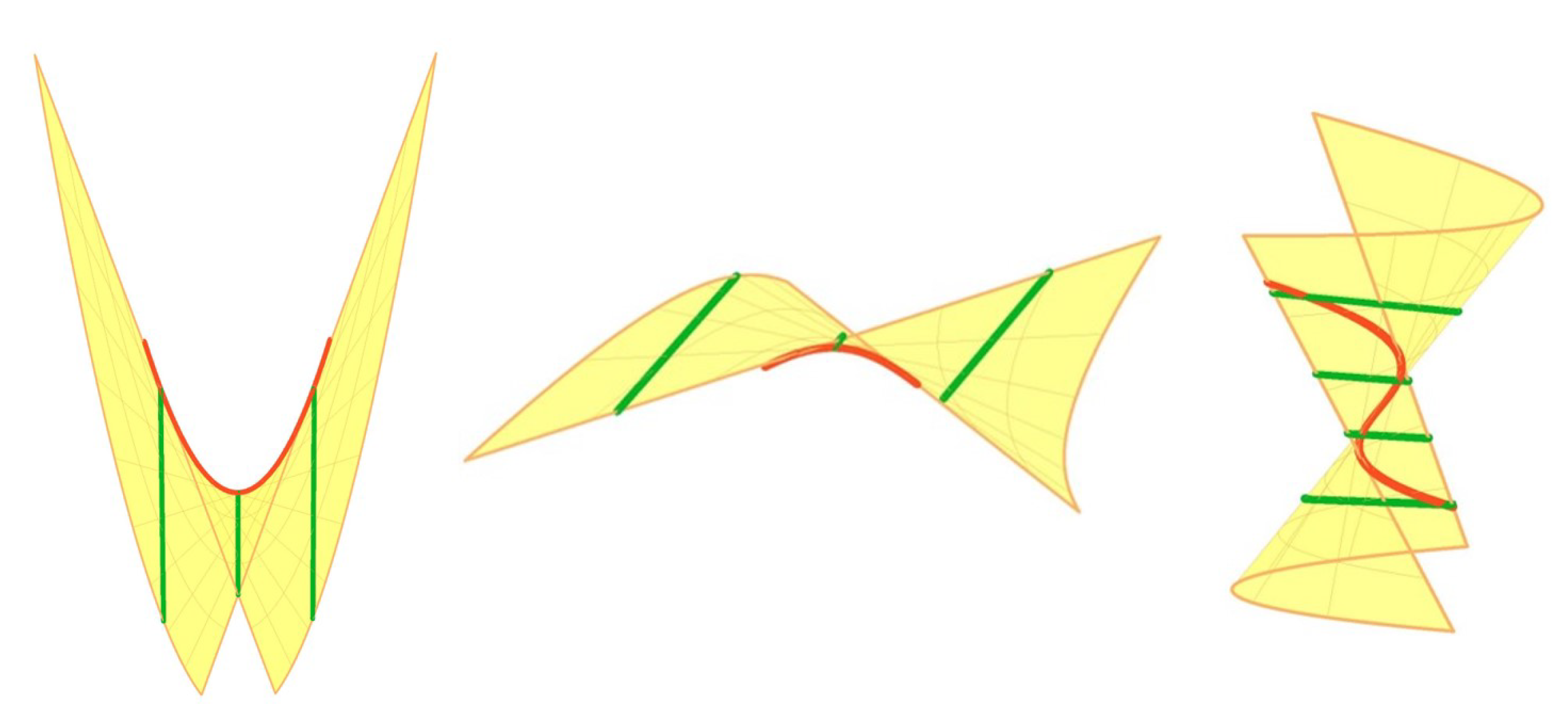
In the following three examples, we calculate the involutes of pseudo-null curves which were classified by Walrave [
18].
Example 1. The only pseudo-null curve with the pseudo-torsion is the curve It is a (Euclidean) parabola in the lightlike plane with the axis of null direction , therefore a circle in a lightlike plane. The developable tangent of is parametrized byand its involutes are(see Figure 1 (left)). The involutes are intersections of planes and (), and therefore null straight lines. Example 2. The only pseudo-null curve with the non-zero constant pseudo-torsion is the curve in the lightlike plane The tangent developable of is parametrized byand its involutes are(see Figure 1 (middle)). The involutes are intersections of planes and , , and therefore null straight lines. Example 3. Let be the pseudo-null curve It is a pseudo-null curve lying in the lightlike plane . Its pseudo-torsion is . The tangent developable of is parametrized by It represents the lightlike plane . The involutes of c arewhere (see Figure 1 (right)). Remark 1. The intrinsic geometry of curves in a lightlike (isotropic) plane can be considered in terms of geometry of curves in the isotropic plane as developed in, e.g., [19]. Isotropic plane is a vector space equipped with a degenerate scalar product , for . There is a unique isotropic direction in generated by . For a non-isotropic curve , , the isotropic Frenet frame is defined by the fields and which are orthogonal with respect to . The isotropic curvature is defined by the Frenet formulasand expressed by . The induced metric of a lightlike plane in Lorentz–Minkowski 3-space is a degenerate of index 1, and as such can be related to the metric of . Let us describe the pseudo-null curve (7) in Example 1 which lies in the lightlike plane π given by , as a curve in the isotropic plane . The local coordinates in the plane π can be introduced by, for instance, , . Then , , or in the local coordinates , . Therefore the isotropic curvature of c is equal to Since the curve (7) has constant isotropic curvature, it is a circle in , as stated in Example 1. Thus the curvature of a curve c appears to be more informative than its vanishing pseudo-torsion τ. Theory of curves of Lorentz–Minkowski space lying in the lightlike planes can be generally related to theory of curves in which is considered in [20]. 4. Reconstruction by the Involutes
Once we have proved that the involutes of a pseudo-null curve are null straight lines, we address with the inverse process that can be expressed with the next
Question. For a given null straight line, is it possible to find a pseudo-null curve whose involute is the initial straight line?
We follow the notation of
Section 3. The given involute
is a null straight line. Let
be a null frame and let
be the Frenet frame of
c. In order to understand the relation between both curves, first we notice that starting from definition (
4), the initial curve
c can be expressed as
We express the frame
in terms of the Frenet frame of
c. First, let
. On the other hand, since
then
, where
,
. We write the second vector
B as
. From the condition
it follows that
. Furthermore, since
B is a null vector,
, it follows
. Therefore,
B is
Finally, we determine the third vector
C. The spacelike vector
C is given by
, and therefore
Notice that here we used the assumption
. If the opposite vector is obtained, then we would frame a straight line accordingly by
. Now, direct calculation implies that the curvatures of the involute are
Observe that vanishing of
was expected because
is a straight line (Corollary 1). Returning with the previous computations, from the expression of
A and
C,
Furthermore, eliminating
from the identities of
and
,
for a certain function
. We are now in position to answer to the problem of reconstruction of the pseudo-null curve whose involute is prescribed. We change the perspective about what is given; it is the involute and we are looking for the initial pseudo-null curve.
Theorem 2. Let be a null straight line framed by a null frame . Then a curve parametrized byis a pseudo-null curve with as its involute, where is a constant and a function that satisfies the first order linear ordinary differential equation Furthermore, all these planar curves are contained in lightlike planes orthogonal to .
Proof. From (
16) it follows that
where the last equality is obtained by substituting
from (
17). Therefore,
Since
is a unitary spacelike vector and
a null vector, the curve
e is a pseudo-null curve parametrized by arc length. Its tangents are orthogonal to tangents of
,
. Finally, we check whether an involute of
e is the initial null straight line
. Using (
16) and (
18), an involute of
e for an arbitrary constant
is
Thus if , we obtain the initial curve as required.
For the last statement, we can assume that A is constant because is a straight line. Then it suffices to observe that all the velocity vectors are orthogonal to A. □
The previous theorem provides, for a given constant , a family of curves regulated by the function with a straight line as their involute. Their pseudo-torsion is calculated as follows:
Corollary 2. The pseudo-torsion of curves e is given by Proof. Using (
18) for
and (
19) for
we obtain
Since
, by using the Frenet formula
we obtain
which implies the required formula. □
Corollary 3. The pseudo-torsion τ of the pseudo-null curves e does not depend on the initial framings of the null straight line .
Proof. Let
be a null straight line framed by different null frames
and
. Then
Furthermore,
. Now, Equation (
21) implies
and we have
Therefore (
20) implies the statement. □
From the previous Corollary we can conclude that different null framings of a given parametrization of a null straight line generate congruent pseudo-null curves e for a given constant .
In the last part of this section, we have shown examples of how Theorem 2 can be employed. We begin by observing that among various frames for a null straight line, frames with fields
constant are of special interest due to their simplicity. They satisfy also
,
, and have
. The initial pseudo-null curve can be easily reconstructed by (
16) with
satisfying
In this case, the pseudo-torsion of the initial pseudo-null curve
is given by (
20)
Notice that the pseudo-torsion is related only to the curvature of the null straight line. In previous Examples we have , , which give , , , respectively. Different straight lines with the same curvature , even more, with curvatures that are equal to up to a multiplicative constant, generate congruent pseudo-null curves.
Proposition 3. Let be a null straight line, , where A is a constant vector (direction vector). It is always possible to frame with a null frame consisting of constant vectors.
Proof. If we prescribe , then a frame for c satisfies which implies the conclusion. □
Remark 2. Notice that not every frame having the vector A constant needs to be such. If we prescribe , then we will have not constant. For example, for with we obtain , . Notice also that a frame consisting of constant vectors is not unique.
A (single) null straight line can generate different pseudo-null curves
e, depending on its parametrization. However, in Corollary 3 we have seen that a given parametrization
of a straight line generates congruent pseudo-null curves regardless of its null framings. Now we also examine relative positions of pseudo-null curves
e regarding different null frames of
. A way for obtaining null frames for a given
is explained in [
16]. Considering any two positive smooth functions
and
, any other null frame of a null curve is given by
Theorem 3. Let be a null straight line framed by a null frame , where is constant. Let be the pseudo-null curve with as its involute. Then the curve for the null frame (22) with as the involute is related to in the following waywhere is a constant. Proof. For the null frame where
is constant, we have
. If we write
(see (
21)), then
and
For the null frame
we have from Theorem 2
For the null frame
, we have
Let
. Then using (
17) for
and
,
If we now replace the values of
and
from (
23) in the above expression, we deduce
, so
f is constant and completes the proof. □
We point out that if in the above theorem is not constant, then . With the same computations, we obtain that and it is not possible to obtain an simple expression for f.
We finish this section with examples of the use of Theorem 2 on the curves obtained in examples presented in
Section 3.
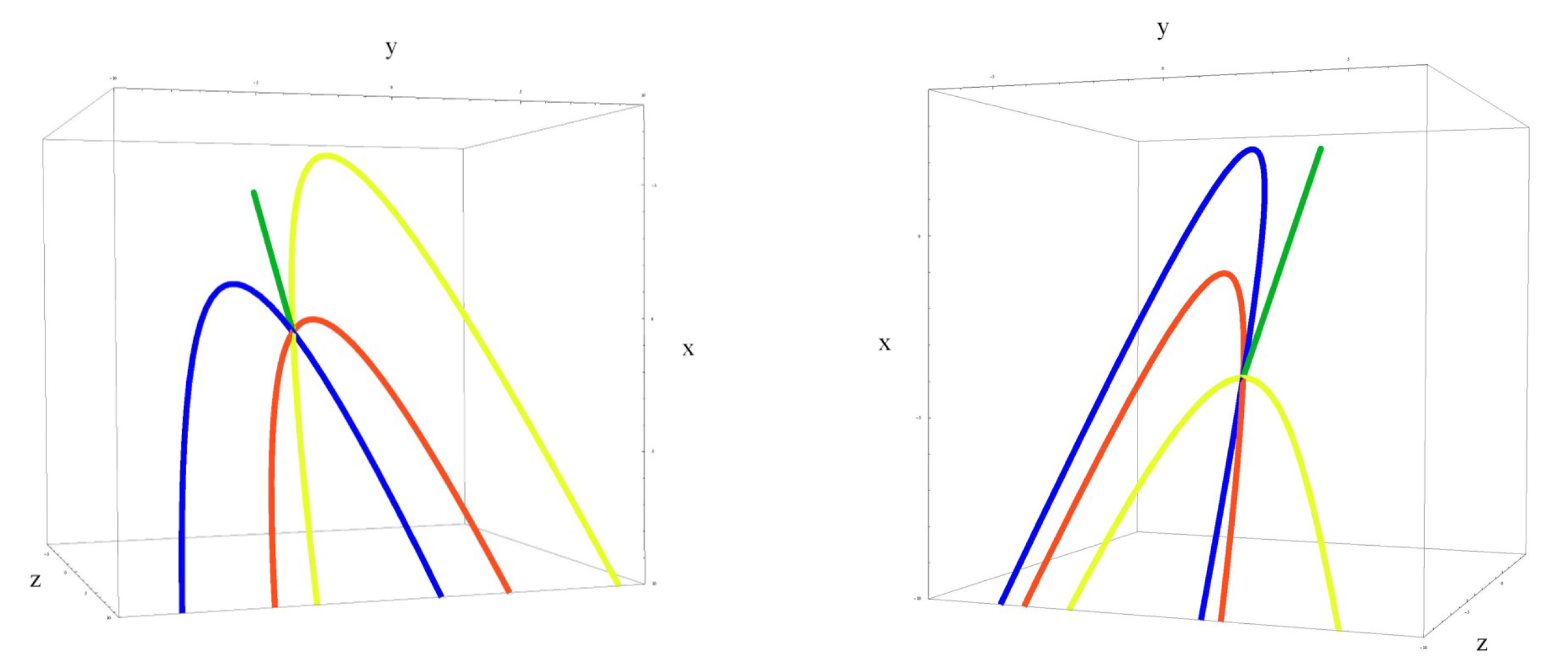
Example 4. We revisit Example 1. Consider the null straight linewhere , parametrized in (9). Then . If we take and the null framethen . Equation (17) is whose solution is , . Then is the involute of the curvesChoosing we recover the initial curve of Example 1. We could also consider another null frame with and non-constant vector fields, Here the curvatures are , . Equation (17) reduces to whose solution is , . The straight line is the involute of the curves For , the initial curve of the Example 1 is obtained. See Figure 2 (left). Regarding different frames chosen, we can notice that they are related by , in (22). Theorem 3 gives the mutual relation of the corresponding evolutes. Example 5. Consider the null straight lineof Example 2. The computation of gives Then we take and the frame Then . Equation (17) is , and its solution is . Then is the involute of the family curves, The choice gives the initial curve (10). See Figure 2 (right). Let us consider another frame for this null straight line. We choose another constant null frame Then again we have , with all other curvatures vanishing, and , , as for the first frame. Then is the involute of the following curves The choice generates the initial curve, see Figure 2 (right). We can notice that frames are related by in (22). Theorem 3 gives Example 6. Consider the null straight linewhere , given in (15). The computation of gives First, consider framed by Then , . Equation (17) reduces to whose solution is . Then is the involute of the family of curves The choice gives the initial curve (13), see Figure 3 (left). For the second frame for , we chose the vectors B and C that are not constant. So, letwhere m and are constant. Then and Equation (17) reduces to whose solution is Then is the involute of the curve where it is The choice and gives the initial curve (13), see Figure 3 (right). Given frames for the null straight line are related by the functions , . Theorem 3 gives their mutual relation.


