Article

A Functional Interpolation Approach to Compute Periodic Orbits in the Circular-Restricted Three-Body Problem

1
Aerospace Engineering, Texas A&M University, College Station, TX 77843, USA
2
Mission Design and Navigation Section, Jet Propulsion Laboratory, California Institute of Technology, Pasadena, CA 91125, USA
*
Author to whom correspondence should be addressed.
Mathematics 2021, 9(11), 1210; https://doi.org/10.3390/math9111210
Submission received: 10 May 2021 / Revised: 24 May 2021 / Accepted: 25 May 2021 / Published: 27 May 2021
(This article belongs to the Section Functional Interpolation)

Abstract

:
In this paper, we develop a method to solve for periodic orbits, i.e., Lyapunov and Halo orbits, using a functional interpolation scheme called the Theory of Functional Connections (TFC). Using this technique, a periodic constraint is analytically embedded into the TFC constrained expression. By doing this, the system of differential equations governing the three-body problem is transformed into an unconstrained optimization problem where simple numerical schemes can be used to find a solution, e.g., nonlinear least-squares is used. This allows for a simpler numerical implementation with comparable accuracy and speed to the traditional differential corrector method.

1. Introduction

According to Poincaré, “periodic orbits” provide the only gateway into the otherwise impenetrable domain of nonlinear dynamics. With the advent of space exploration, periodic orbits have become an indispensable part of missions in space. The amazing fish-like Apollo orbit was the first three-body orbit used for space missions. The second three-body orbit used for space missions was the Halo orbit, discovered by Robert Farquhar in his Ph.D. thesis [1] under John Breakwell [2]. In 1978, Farquhar convinced NASA and led the International Sun-Earth Explorer 3 mission (ISEE3) to study the Sun from a Halo orbit around the Earth’s L1 Lagrange point. Farquhar’s original idea was to place a satellite in Halo orbit around the Lunar L2 for telecommunication support for the backside of the Moon. Today, this is indeed part of NASA’s planned return of humans to the Moon in the next few years.
Computing Halo orbits, and finding nonlinear periodic orbits in general, has become an important part of modern mission design. This paper introduces a novel, simple, and efficient method for finding periodic orbits using the Theory of Functional Connections (TFC) [3,4]. First, we review perhaps the most popular standard method for computing periodic orbits: the differential correction method (also called shooting method), such as presented by Kathleen Howell [5]. One begins with an approximate solution obtained typically from normal form expansions. Using the variational equation, the guess solution is iteratively corrected for periodicity. Assuming that the initial guess is in a reasonable basis of attraction to a periodic orbit, the process converges to a periodic orbit. In Hamiltonian systems, periodic orbits typically occur in one-parameter families. Often, there are multiple families nearby. Hence, the convergence may not always lead to the desired orbit. Moreover, control over the specific features of the periodic orbit, such as its period or energy, requires additional work—for example, using continuation methods to reach the exact orbit desired. Using TFC, the functional interpolation theory, a simpler formulation and more efficient algorithm for finding periodic orbits is possible.
With this work, we removed the need for a shooting method by analytically embedding the boundary conditions in the solution space using TFC [3,4]. These expressions, which will be explicitly derived in the following sections, transform a differential equation subject to constraints into an unconstrained problem, reducing the whole solution function space to only the subspace satisfying the constraints. This method drastically simplifies the problem and allows for simple numerical implementation; in our case, we utilize a nonlinear least-squares technique.

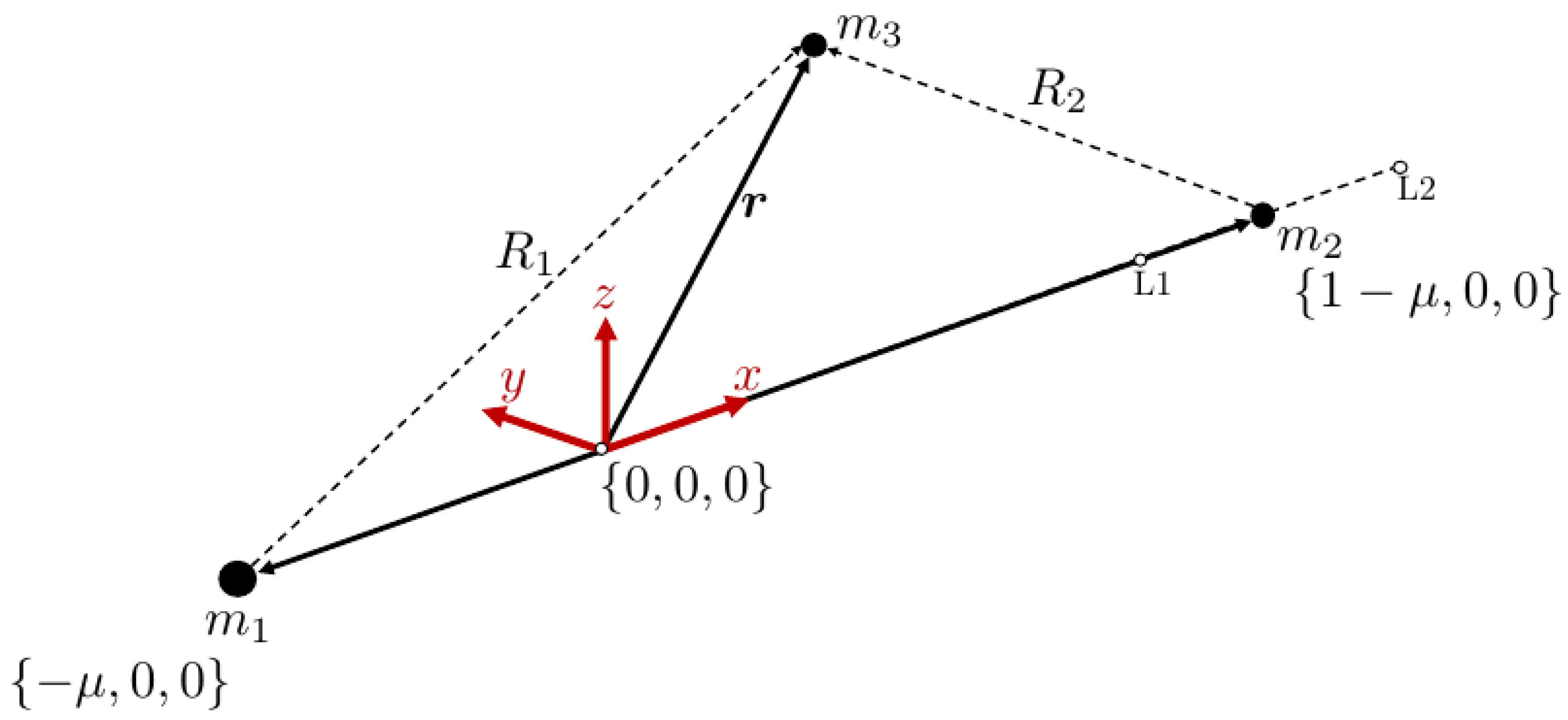
2. Circular-Restricted Three-Body Problem

The circular-restricted three-body problem (CR3BP) is a dynamical model used to describe the motion of a particle r = { x , y , z } T of negligible mass under the influence of a primary body of mass m 1 and the secondary body of mass m 2 . Furthermore, the orbits of m 1 and m 2 are subject to circular motion about the system’s barycenter and lie in the x-y plane as depicted in Figure 1. Following this, the system can be non-dimensionalized by the following scaled units: unit mass is defined as m 1 + m 2 ; unit length is taken as the separation between m 1 and m 2 ; the unit time is chosen such that the orbital periods of m 1 and m 2 about the system’s barycenter are 2 π . By following these steps, the system can be reduced to a single parameter called the mass parameter, μ , where,
μ = m 2 m 1 + m 2
From this, we define the terms μ 1 and μ 2 based on Equation (1) as
μ 1 = 1 μ and μ 2 = μ .
Using this definition of the system, the equations of motion can be derived in the rotating frame, leading to the following system of equations:
x ¨ 2 y ˙ = Ω x y ¨ + 2 x ˙ = Ω y z ¨ = Ω z
such that the shorthand dot notation is used to signify a derivative with respect to time (e.g., x ˙ : = d x d t ). Additionally, Ω is defined as
Ω ( x , y , z ) : = 1 2 ( x 2 + y 2 ) + 1 μ R 1 + μ R 2 + 1 2 ( 1 μ ) μ
where R 1 = ( x + μ ) 2 + y 2 + z 2 and R 2 = ( x + μ 1 ) 2 + y 2 + z 2 are the distances to the primaries. Furthermore, the equations of motion are Hamiltonian and independent of time and, thanks to Noether’s theorem, have an energy integral of motion E , where, in the celestial mechanics community, the Jacobi constant is used, which is C : = 2 E and given as
C = 2 Ω ( x ˙ + y ˙ + z ˙ ) = ( x 2 + y 2 ) + 2 1 μ R 1 + 2 μ R 2 + ( 1 μ ) μ ( x ˙ + y ˙ + z ˙ ) .
Moving forward, we solve the dynamics defined by the system of equations in Equation (2) such that the orbit is at a fixed energy level (or rather Jacobi constant) using Equation (4). For our implementation, it is useful to define the residuals of these equations:
0 = F x : = x ¨ 2 y ˙ Ω x
0 = F y : = y ¨ + 2 x ˙ Ω y
0 = F z : = z ¨ Ω z
0 = F c : = ( x 2 + y 2 ) + 2 1 μ R 1 + 2 μ R 2 + ( 1 μ ) μ ( x ˙ + y ˙ + z ˙ ) C
Next, we generate analytical expressions for the states to guarantee a periodic orbit.
However, before moving forward, it is necessary to summarize the major steps of the differential corrector method [5], since this technique is used as a baseline to compare results with the proposed method. In general, the differential correction method can be classified as a shooting method since it relies on transforming the boundary-value problem into an initial-value problem where the initial conditions are iteratively adjusted. First, unlike the the proposed technique, the differential correction method can take advantage of the symmetry of the orbits about the x-z plane, which leads to the following conditions:
X ( 0 ) = x 0 , 0 , z 0 , 0 , y ˙ 0 , 0 T
and
X ( T / 2 ) = x , 0 , z , 0 , y ˙ , 0 T
where Equations (9) and (10) represent the initial state and the state at half of the period, T, where the orbit crosses the x-z plane (the sign of the y variable). Therefore, the equations of motion only need to be propagated to this sign change. At this point, if the values of | x ˙ | and | z ˙ | are zeros within an acceptable tolerance (Ref. [5] uses 10 8 ), then the orbit is considered periodic. If they are not, the initial conditions are updated by determining
δ X ( 0 ) = δ x 0 , 0 , δ z 0 , 0 , δ y ˙ 0 , 0 T
and adding the result to Equation (9). The values in Equation (11) are determined by the state transitions matrix calculated in the propagation step and the fact that the only changes to state should be the variables x ˙ and z ˙ , which should be equal to the negative of their values at T / 2 , i.e., δ x ˙ should be x ˙ (see Refs. [2,5] for the detailed equations). After updating the initial conditions, the equations of motion are propagated again and the process continues until the periodic conditions are met.

3. Solving the Problem Using the Theory of Functional Connections Framework

The numerical technique to solve differential equations based on the Theory of Functional Connections [4] has produced machine error accuracy within milliseconds for both linear and nonlinear [6] differential equations for a wide array of constraint cases. In fact, several works have already adopted the TFC framework to solve mathematical problems including hybrid systems [7], optimal control problems [8,9], quadratic and nonlinear programming [10], and other applications [11,12].
The foundation of this approach is the ability to derive a class of functionals, called constrained expressions, which have the characteristic of always analytically satisfying assigned linear constraints. Using these constrained expressions, the differential equation can be transformed into an algebraic expression that can ultimately be solved via a variety of optimization techniques. In general, the TFC methodology provides functional interpolation by embedding a set of k linear constraints. Let g ( t ) be a general function in our unconstrained function space, G. We define next the subspace, Γ G , of constrained functions, x ( t , g ( t ) ) , subject to these k linear constraints written as the following functional:
x ( t , g ( t ) ) = g ( t ) + j = 1 k ϕ j ( t )   ρ j ( t , g ( t ) ) ,
where g ( t ) is a free function, and ϕ j ( t ) are switching functions—by definition, a function is equal to 1 when evaluated at the constraint it is referencing, and equal to 0 when evaluated at all other constraints. In our case, the switching functions are composed of a set of mutually linearly independent functions called support functions, s k ( t ) , with unknown coefficients α i j , such that ϕ j ( t ) = s i ( t )   α i j ; however, the switching functions can be very general depending on the nature of the original function space, G.
Furthermore, ρ j ( t , g ( t ) ) are called projection functionals, since they are derived by setting the constraint function equal to zero and replacing x ( t ) with g ( t ) . The following step-by-step procedure can be used to derive a constrained expression from Equation (12):
1.
Choose k linearly independent support functions, s k ( t ) .
2.
Write each switching function as a linear combination of the support functions with k unknown coefficients.
3.
Based on the switching function definition, write a system of equations to solve for the unknown α i j coefficients.

3.1. Derivation of Constrained Expression

First, since, in our problem, the orbital period is unknown, let us normalize the time domain from t [ 0 , T ] , where t 0 = 0 ,   t f = T , to τ [ 1 , + 1 ] , where τ 0 = 1 ,   τ f = + 1 . The simplest mapping is a linear one as follows:
τ ( t ) = τ 0 + τ f τ 0 t f t 0 ( t t 0 ) t = t 0 + t f t 0 τ f τ 0 ( τ τ 0 ) .
where we defined the following coefficient term of the derivative of τ with respect to t. (Note: here, we define the coefficient term as the square of b in order to ensure that the ratio is always positive, i.e., the problem domain is always consistent. This is important in numerical implementation when solving for the value of b.)
b 2 : = d τ d t = τ f τ 0 t f t 0 ,
Now, we write the constrained expression in terms of this new variable τ . Let us define the position vector of the spacecraft as r ( τ ) = { r x ( τ ) , r y ( τ ) , r z ( τ ) } T = { x ( τ ) , y ( τ ) , z ( τ ) } T . Since the problem presented in this paper is to find periodic orbits in the CR3BP, we can use the TFC expression to satisfy the following constraints:
r i ( τ 0 ) = r i ( τ f ) = α i and r i ( τ 0 ) = r i ( τ f ) = β i b 2
or, in other words, the trajectory must return to the initial state at some period. Since the constraints for each component of the vector r i ( τ ) are of the same form, Equation (12) can be easily adapted to the vector form:
r i ( τ , g i ( τ ) ) = g i ( τ ) + j = 1 k ϕ j ( τ )   ρ j ( t , g i ( τ ) ) ,
Following the process detailed in the prior section, one must first choose the support functions s k ( τ ) . For these specific constraints, the support functions are defined in the same manner as Ref. [9], where s k ( τ ) = τ ( k 1 ) . Now, the definition of the switching functions is used to produce a set of equations. For example, the first switching function has the four following equations:
ϕ 1 ( τ 0 ) = 1 , ϕ 1 ( τ f ) = 0 , ϕ 1 ( τ 0 ) = 0 , and ϕ 1 ( τ f ) = 0 ,
These equations are expanded in terms of the support functions:
ϕ 1 ( τ 0 ) = ( 1 ) · α 11 + ( τ 0 ) · α 21 + ( τ 0 2 ) · α 31 + ( τ 0 3 ) · α 41 = 1 ϕ 1 ( τ f ) = ( 1 ) · α 11 + ( τ f ) · α 21 + ( τ f 2 ) · α 31 + ( τ f 3 ) · α 41 = 0 ϕ 1 ( τ 0 ) = ( 0 ) · α 11 + ( 1 ) · α 21 + ( 2 τ 0 ) · α 31 + ( 3 τ 0 2 ) · α 41 = 0 ϕ 1 ( τ f ) = ( 0 ) · α 11 + ( 1 ) · α 21 + ( 2 τ f ) · α 31 + ( 3 τ f 2 ) · α 41 = 0
which can be written in matrix form as
1 τ 0 τ 0 2 τ 0 3 1 τ f τ f 2 τ f 3 0 1 2 τ 0 3 τ 0 2 0 1 2 τ f 3 τ f 2 α 11 α 21 α 31 α 41 = 1 0 0 0 .
The same is done for the other three switching functions to produce a set of equations that can be solved by matrix inversion, where τ 0 = 1 and τ f = 1 .
1 τ 0 τ 0 2 τ 0 3 1 τ f τ f 2 τ f 3 0 1 2 τ 0 3 τ 0 2 0 1 2 τ f 3 τ f 2 α 11 α 12 α 13 α 14 α 21 α 22 α 23 α 24 α 31 α 32 α 33 α 34 α 41 α 42 α 43 α 44 = 1 0 0 0 0 1 0 0 0 0 1 0 0 0 0 1 .
that is,
α 11 α 12 α 13 α 14 α 21 α 22 α 23 α 24 α 31 α 32 α 33 α 34 α 41 α 42 α 43 α 44 = 1 τ 0 τ 0 2 τ 0 3 1 τ f τ f 2 τ f 3 0 1 2 τ 0 3 τ 0 2 0 1 2 τ f 3 τ f 2 1 = 1 4 2 2 1 1 3 3 1 1 0 0 1 1 1 1 1 1 .
This leads to the switching functions,
ϕ 1 ( τ ) = 1 4 2 3 τ + τ 3 ϕ 2 ( τ ) = 1 4 2 + 3 τ τ 3 ϕ 3 ( τ ) = 1 4 1 τ τ 2 + τ 3 ϕ 4 ( τ ) = 1 4 1 τ + τ 2 + τ 3 .
By their definition, the projection functionals are
ρ 1 = α i g i ( τ 0 ) ρ 2 = α i g i ( τ f ) ρ 3 = β i b 2 g i ( τ 0 ) ρ 4 = β i b 2 g i ( τ f )
Collecting these terms in the form of Equation (15), the constrained expression and its derivatives can be expressed as
r i ( τ , g i ( τ ) ) = g i ( τ ) + ϕ 1 ( τ ) α i g ( τ 0 ) + ϕ 2 ( τ ) α i g ( τ f )   + ϕ 3 ( τ ) β i b 2 g ( τ 0 ) + ϕ 4 ( τ ) β i b 2 g ( τ f )
In order to use this expression in our differential equation, we need to utilize the mapping parameter b from Equation (14), where
d r i d t r ˙ i = b 2 d r i d τ r i .

3.2. Definition of the Free Function g j ( τ )

For this application, let the free function be expressed as a linear combination of basis functions multiplied with unknown coefficients according to
g i ( τ ) = j = 1 m a i j   T j ( τ ) = ξ i T   h ( τ )
where h R m is a vector of the basis functions T j ( τ ) and ξ i R m is the unknown coefficient vector associated with the ith vector component. Like the original work on the solution of ordinary differential equations with TFC [6], we utilize Chebyshev orthogonal polynomials in the paper. The orthogonal polynomial representations are generally preferred due to their approximating and convergence properties. For example, Chebyshev polynomials generate a function that minimizes the maximum error in its application, and, therefore, they are well suited to approximating other functions [13,14].
However, due to the structure of the constrained expression, the free functions can be defined by a variety of function approximation methods, including other orthogonal polynomial sets and techniques in the field of machine learning. In fact, the application to neural networks (NN) was studied in Ref. [11], and promising results have been obtained by using the Extreme Learning Machine (ELM) [15], which is a single-layer feed-forward NN. The interested reader is directed to Ref. [16] for an in-depth look at the ELM implementation with TFC and Ref. [17] for applications of this technique to problems in spaceflight.

3.3. Discretization of the Domain

In order to solve problems numerically, the problem domain (and therefore the basis function domain) must be discretized. Since this article uses Chebyshev orthogonal polynomials, an optimal discretization scheme is the Chebyshev–Gauss–Lobatto nodes [18,19] shown in Equation (18). For N + 1 points, the discrete points are calculated as
τ k = cos k π N for k = 0 , 1 , 2 , , N .
Compared with the uniform distribution, the collocation point distribution results in a much slower increase in the condition number of the matrix to be inverted in the least-squares as the number of basis functions, m 2 , increases. The collocation points can be realized in the problem domain through the relationship provided in Equation (13).

3.4. Solution of the Resulting Algebraic Equation

By defining g i ( t ) according to Equation (17), our definition of Equations (2) and (3) is converted into four algebraic equations:
F ˜ i ( τ , Ξ ) = 0   for   i = x , y , z , c
defined from Equation (5) through Equation (8). Note that the tilde symbol (∼) is used to signify that the differential Equation (5) through Equation (8) have been transformed into a new set of equations with embedded constraints. Additionally, Ξ represents the unknown parameters of this transformed set of equations, and these are defined in the following equations.
Next, we evaluate the three differential equations and one algebraic equation given by Equation (19) at the discretization points to construct a loss vector of the residuals of these equations.
L i ( Ξ ) = F ˜ i ( τ 0 , Ξ ) , , F ˜ i ( τ k , Ξ ) , , F ˜ i ( τ f , Ξ ) T = 0 T
with the total loss vector of
L ( Ξ ) = L x T ( Ξ ) , L y T ( Ξ ) , L z T ( Ξ ) , L c T ( Ξ ) T = 0 4 N × 1 T
where the unknown vector, of size composed of 3 m + 7 terms, is defined as
Ξ = ξ x T , ξ y T , ξ z T , α T , β T , b T = 0 T
Since the governing dynamics of the circular-restricted three-body problem are nonlinear, the unknown parameters occur nonlinearly in the loss vector, Equation (20). Therefore, a nonlinear least-squares technique was utilized using Equation (21) to update the parameters:
Ξ k + 1 = Ξ k + Δ Ξ k
where Equation (22) is the classical least-squares equation using the Moore–Penrose inverse of the Jacobian of Equation (20):
Δ Ξ k = J T ( Ξ k )   J ( Ξ k ) 1 J T ( Ξ k )   L ( Ξ k ) ,
This nonlinear least-squares method, known as the Gauss–Newton algorithm, is a modification of Newton’s method for finding a minimum of a function—in our case, minimizing the sum of the squared residual values in Equation (20).
The iteration continues until one of the following conditions is met:
max | L ( Ξ k ) | < ε max | Δ Ξ k | < ε ,
based on the user defined tolerance, ε , or the iteration exceeding some user-defined maximum.

4. Numerical Test

In the numerical implementation, all Jacobians were calculated using the JAX package [20,21] utilizing automatic differentiation [22]. In the nonlinear least-squares steps, NumPy’s pinv() was used to calculate the Moore–Penrose pseudo-inverse through singular-value decomposition (SVD). Additionally, a just-in-time compiler was used to optimize the code. All timing was handled by the process_time() from the Python package time. For all problems, we considered the Earth–Moon system with the parameters given in Table 1. Additionally, for the TFC implementation, the parameters used are summarized in Table 2.

4.1. Initialization

For all numerical tests, the unknown vector must be initialized. First, the terms ξ x , ξ y , and ξ z were all initialized by a null vector, which ultimately represents the simplest interpolating expression for the state variables. This initialization represents the worst-case scenario when there is no estimation of the trajectory, but just fitting the constraints. Next, the other unknown values of α , β , and b (which are associated with the position, velocity, and the period of the orbit) were initialized using Richardson’s third-order analytical method for Halo-type periodic motion [23]. This initialization was used to find the first orbit of the specified Jacobi constants. For the following orbits, the desired Jacobi constant was incrementally increased, and the converged values from the prior Jacobi constant level were used to initialize each following step.
The same process was utilized for the differential corrector method [5], which was implemented to compare with TFC. In the differential corrector inner-loop, the desired Jacobi constant was obtained by an iterative least-squares approach to update the initial guess.

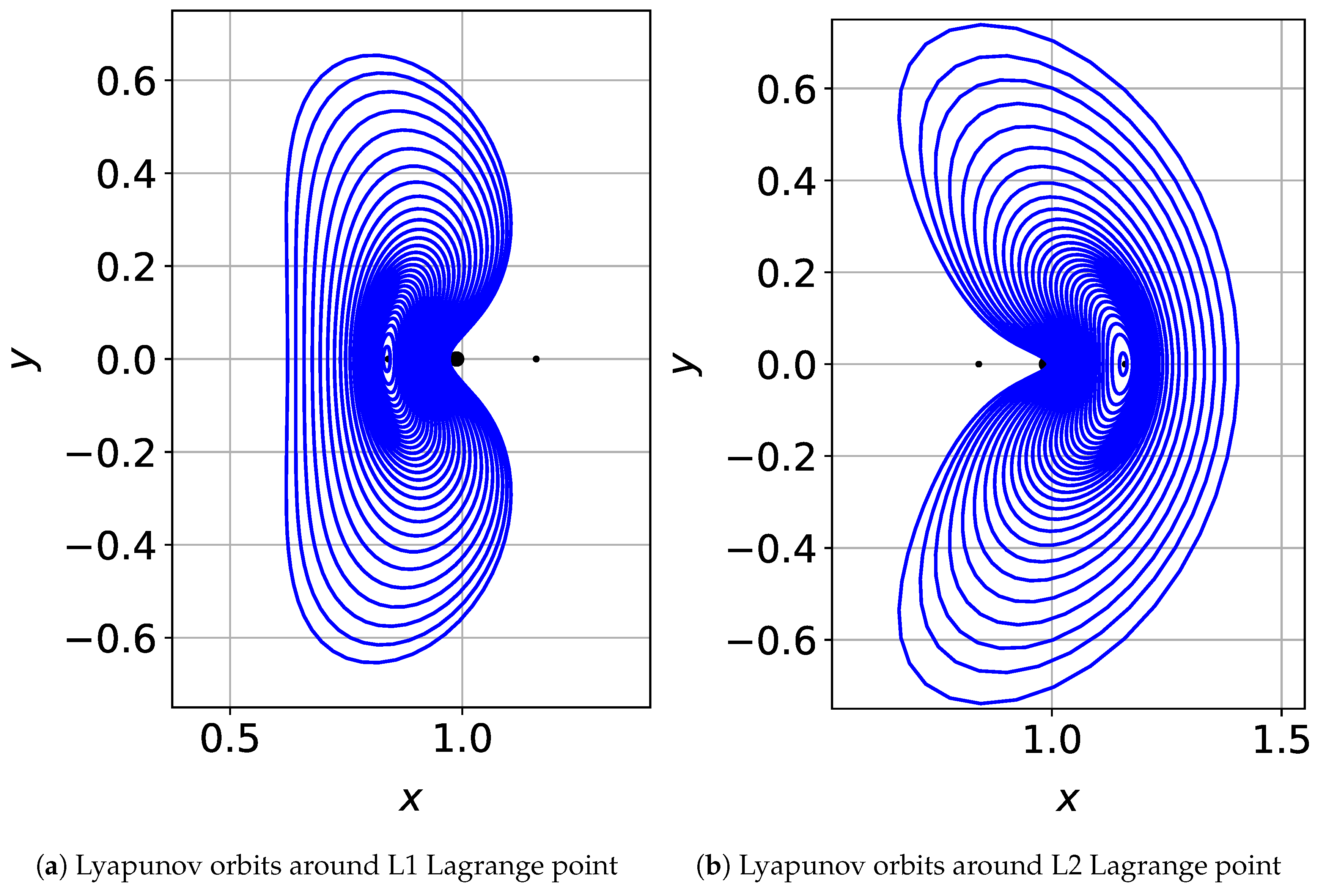
4.2. Lyapunov Orbits

First, the TFC method was used to explore the computation of Lyapunov orbits, which lie in the x-y plane, the orbital plane of the two primaries. For our test, the Lyapunov orbits were computed over a range of Jacobi constants, starting close to the equilibrium point’s specific energy levels and terminating at a Jacobi constant of 2.92. The associated trajectories for the orbits around L1 and L2 are provided in Figure 2a,b.
For the solution of Lyapunov orbits, it was important to transform the time for orbits of lower Jacobi constants, i.e., orbits closer to the secondary body, m 2 . This was done by the time transformation from Ref. [5], where t ζ , such that
d t d ζ = R 2 .
This produces the following chain of transformations t ζ τ , or rather [ 0 , T ] [ 0 , ζ f ] [ 1 , + 1 ] , which produces the final transformation:
r ˙ i ( t ) = d r i d t = d r i d τ · d τ d ζ · d ζ d t = b 2 R 2 r i ( τ )
To stress the importance of this scaling, Figure 3 shows both the scaled and non-scaled TFC solution for Lyapunov orbits around L1 (Figure 3a) and L2 (Figure 3b).
It can be seen that this scaling has a drastic effect on the accuracy of the converged solution. For orbits around L1, without scaling, significant accuracy loss is observed starting at a Jacobi constant of around 3.15. For orbits around L2, this accuracy reduction starts at a Jacobi constant of around 3.06, but is just as drastic.
Additionally, a comparison with the differential corrector method is provided in terms of speed and accuracy. Figure 4 compares the residuals for both methods, where it can be seen that the TFC approach is around two orders of magnitude more accurate than the differential corrector at higher Jacobi constants. Furthermore, the computation of the TFC solution is slightly faster, a little over 0.25 s in the extreme case, as displayed in Figure 5.
To further understand the computation time associated with the TFC approach, consider the computational breakdown given in Figure 6. Additionally, the statistics associated with this breakdown, in terms of mean and standard deviation, are given in Table 3. In the TFC method, the three major computations in each nonlinear least-squares iteration are evaluating the loss vector, the Jacobian, and the least-squares. Figure 6 shows that around 77% of the total computation time is associated with the least-squares portion. This should come as no surprise since the Jacobian is a 4 N × 2 m matrix— 560 × 260 for this problem.
While the least-squares, i.e., matrix inversion, is the main bottleneck with the computational efficiency, a marginal speed gain could be achieved by removing the reliance on automatic differential through JAX [20,21] for the computation of the loss vector and Jacobian. Admittedly, these two could be “hard-coded” since the partial derivatives populating the Jacobian can be analytically derived. However, the speed gain associated with this is unknown and should be the focus of future implementations and numerical tests.
Similar to the L1 Lagrange point test, Figure 2a displays the computed trajectories around the L2 Lagrange point. Additionally, as in Figure 4 and Figure 5, the accuracy and computation time for these tests are provided in Figure 7 and Figure 8. In Figure 7, the TFC method is more accurate, albeit only slightly. At a Jacobi constant level of around 3.00 and above, the differential corrector method does not converge, as shown by the jump in accuracy. At this Jacobi constant level, the TFC method’s accuracy starts to decrease before failing to converge at the Jacobi constant value of 2.92. This drop-off in the accuracy of the TFC method can easily be seen by analyzing Figure 8, where the red box highlights where the TFC method’s max iteration limit is reached. In other words, at the Jacobi constant levels lower than 3.00, the representation of the orbit through the free function composed of Chebyshev polynomials starts to fail.
In both Lyapunov orbits around L1 and L2, the reduction in accuracy can be attributed to the definition of the free function, g ( x ) , not fully capturing the solution space of the trajectory. As the Jacobi constant decreases, the complexity of the trajectory’s shape increases and therefore an increasing number of basis functions is needed. However, contrary to this, increasing the basis terms to more than 130 does not provide a more accurate solution in the numerical implementation. Therefore, when solving lower Jacobi constant level Lyapunov orbits, a different definition of the free function must be used; future effort should focus on exploring other basis types.

4.3. Halo Orbits

Next, the proposed technique was utilized to compute Halo orbits around L1 and L2. These orbits differ from the Lyapunov orbit because they are not restricted to the x-y plane and are therefore three-dimensional. In fact, this family of orbits is a bifurcation of the Lyapunov orbits computed in the previous section and is characterized by “northern” and “southern” bifurcations. However, using the TFC method to compute these Halo orbits, the only difference is in the initialization of the α , β , and b parameters. Additionally, for Halo orbits, the time transformation introduced in Equation (23) was not used because it produced unfavorable convergence properties, i.e., the method would simply converge to the Lyapunov family of orbits. First, we look at the computation of the “northern” family of Halo orbits around L1 and L2, as plotted in Figure 9.
In these plots, we can see that, around the L1 equilibrium point, the method converged to Lyapunov orbits for higher Jacobi constants. However, as the Jacobi constant decreases below 3.025, the method does not converge to a periodic orbit, as shown by the increase in residuals around the Jacobi constant value of 3.025. At the other equilibrium point, L2, the method converges for all Jacobi constant values; however, at values below 3.025, the solution jumps to a circular orbit around the Moon. Therefore, these orbits were not plotted. This “jumping” from the Halo orbit bifurcation to the circle orbit bifurcation is the major drawback with the algorithm in its current state; however, it is noted that the differential corrector approach also suffers from this. The reason that the TFC method exhibits this behavior is that the numerical solution, i.e. the nonlinear least-squares optimization step, has no information on the desired bifurcation. Therefore, the solution becomes closely linked to (1) the initialization of the unknown parameters and (2) the definition of the free function g ( x ) . In other words, the initialized parameters will converge to the closest local minimum.
Like the Lyapunov orbit tests, the loss vector’s maximum residual was recorded and is plotted in Figure 10. For almost all converged solutions, the residuals were on the order of O ( 10 14 ) ; however, around a Jacobi constant level of 3.025, the accuracy decreases for orbits around L1. The convergence for Halo orbits took longer, with some cases taking 8 s, while, on average, the solution time was around 2 s, as shown in Figure 11. Similar to the “northern” Halo orbits plotted in Figure 9, the Halo orbits of the “southern” bifurcation were computed with similar findings and, therefore, omitted from this paper for brevity.

5. Conclusions

In this paper, we implemented a functional interpolation method, based on the Theory of Functional Connections (TFC), to computed periodic orbits, i.e., Lyapunov and Halo orbits, in the circular-restricted three-body problem. The TFC approach allowed for the analytical embedding of the periodic constraint, such that the orbit’s initial and final position and velocity repeated after some period T. This process reduces the search space of the numerical algorithm to only those trajectories satisfying the periodic constraint.
In general, the method produced comparable results to the differential corrector method; however, the ease of implementation of the TFC method provides one benefit. For example, when using the TFC method, the user only needs to code the loss vector, Equation (20), and the parameter update is handled through automatic differentiation. For readers interested in this implementation, the authors direct them to the TFC GitHub (https://github.com/leakec/tfc, accessed on 15 February 2021) [24], where both codes for the Lyapunov (https://github.com/leakec/tfc/tree/main/examples/Hunter_Johnston_Dissertation/Chapter_4/Example_4_8, accessed on 15 February 2021) and Halo (https://github.com/leakec/tfc/tree/main/examples/Hunter_Johnston_Dissertation/Chapter_4/Example_4_9, accessed on 15 February 2021) orbit cases are provided. In addition to the code used to produce the results of this paper, this toolbox provides examples to the solution of a wide variety of ODEs and PDEs.
In all, this work was the first time that the TFC method was utilized to enforce the constraints of periodic orbits. Future work in this area should focus on two major aspects in order to increase speed, accuracy, and robustness of the technique, which are summarized below:
  • Definition of the free function. In this study, Chebyshev orthogonal polynomials were used to define the free function; however, a large number of basis terms were needed to accurately describe the trajectories for both Lyapunov and Halo orbits. One idea to remedy this is to use a hybrid basis composed of terms to capture the periodic and non-periodic portions separately.
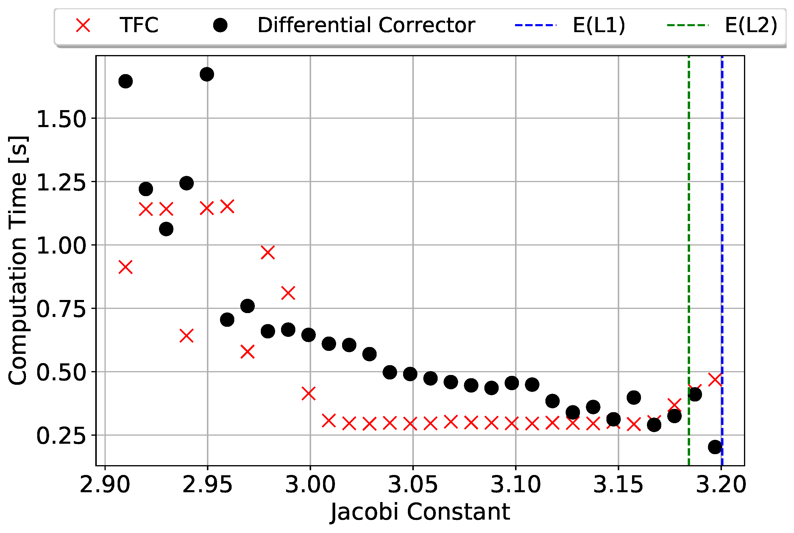
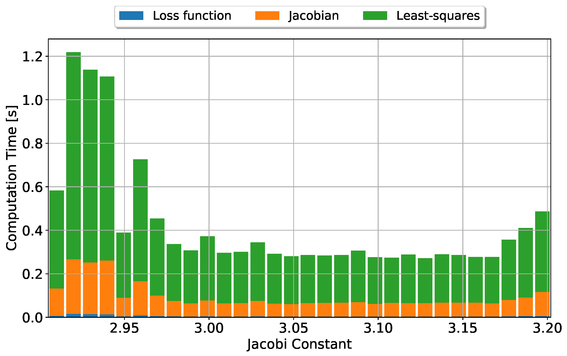
  • Faster least-squares implementation. As seen in Figure 6, the major bottleneck with computation time lies in the least-squares portion, which is an order of magnitude slower than the evaluation of the loss vector and Jacobian combined. The authors acknowledge that a more efficient algorithm than NumPy’s pinv() could be implemented.

Author Contributions

Conceptualization, H.J. and M.W.L.; Formal analysis, H.J.; Methodology, H.J.; Software, H.J.; Supervision, M.W.L. and D.M.; Validation, H.J.; Writing—original draft, H.J. and M.W.L.; Writing—review and editing, H.J., M.W.L. and D.M. All authors have read and agreed to the published version of the manuscript.

Funding

This research was carried out in part at the Texas A&M University, supported by a NASA Space Technology Research Fellowship, Johnston (NSTRF 2019) Grant#: 80NSSC19K1149. This research was carried out in part at the Jet Propulsion Laboratory, California Institute of Technology, under a contract with the National Aeronautics and Space Administration (80NM0018D0004).

Institutional Review Board Statement

Not applicable.

Informed Consent Statement

Not applicable.

Data Availability Statement

The code presented in this paper is available at: https://github.com/leakec/tfc/, accessed on 15 February 2021.

Acknowledgments

Many thanks to JPL and Section 392 for hosting the first author’s summer internship in 2020.

Conflicts of Interest

The authors declare no conflict of interest.

Abbreviations

The following abbreviations are used in this manuscript:
CR3BPcircular-restricted three-body problem
ELMExtreme Learning Machine
ISEE3International Sun-Earth Explorer 3
JPLJet Propulsion Laboratory
NASANational Aeronautics and Space Administration
NNneural networks
NSTRFNASA Space Technology Research Fellowship
ODEordinary differential equation
PDEpartial differential equation
SVDsingular-value decomposition
TFCTheory of Functional Connections

References

  1. Farquhar, R.W. The Control and Use of Libration-Point Satellites. Ph.D. Thesis, Department of Aeronautics and Astronautics, Stanford University, Stanford, CA, USA, 1968. [Google Scholar]
  2. Breakwell, J.V.; Brown, J.V. The ‘Halo’family of 3-Dimensional Periodic Orbits in the Earth-Moon Restricted 3-Body Problem. Celest. Mech. 1979, 20, 389–404. [Google Scholar] [CrossRef]
  3. Mortari, D. The Theory of Connections: Connecting Points. Mathematics 2017, 5, 57. [Google Scholar] [CrossRef] [Green Version]
  4. Leake, C.; Johnston, H.; Mortari, D. The Multivariate Theory of Functional Connections: Theory, Proofs, and Application in Partial Differential Equations. Mathematics 2020, 8, 1303. [Google Scholar] [CrossRef]
  5. Howell, K. Three-dimensional, Periodic, Halo Orbits. Celest. Mech. 1984, 32, 53–71. [Google Scholar] [CrossRef]
  6. Mortari, D.; Johnston, H.; Smith, L. High Accuracy Least-squares Solutions of Nonlinear Differential Equations. J. Comput. Appl. Math. 2019, 293–307. [Google Scholar] [CrossRef] [PubMed]
  7. Johnston, H.; Mortari, D. Least-squares Solutions of Boundary-value Problems in Hybrid Systems. J. Comput. Appl. Math. 2021, 393, 113524. [Google Scholar] [CrossRef]
  8. Furfaro, R.; Mortari, D. Least-squares Solution of a Class of Optimal Space Guidance Problems via Theory of Connections. Acta Astronaut. 2020, 168, 92–103. [Google Scholar] [CrossRef]
  9. Johnston, H.; Schiassi, E.; Furfaro, R.; Mortari, D. Fuel-Efficient Powered Descent Guidance on Large Planetary Bodies via Theory of Functional Connections. J. Astronaut. Sci. 2020, 67, 1521–1552. [Google Scholar] [CrossRef] [PubMed]
  10. Mortari, D.; Mai, T.; Efendiev, Y. Theory of Functional Connections Applied to Nonlinear Programming under Equality Constraints. In Proceedings of the 2019 AAS/AIAA Astrodynamics Specialist Conference, Portland, ME, USA, 11–15 August 2019. Paper AAS 19-675. [Google Scholar]
  11. Leake, C.; Mortari, D. Deep Theory of Functional Connections: A New Method for Estimating the Solutions of Partial Differential Equations. Mach. Learn. Knowl. Extr. 2020, 2, 37–55. [Google Scholar] [CrossRef] [PubMed] [Green Version]
  12. Leake, C.; Johnston, H.; Smith, L.; Mortari, D. Analytically Embedding Differential Equation Constraints into Least Squares Support Vector Machines Using the Theory of Functional Connections. Mach. Learn. Knowl. Extr. 2019, 1, 1058–1083. [Google Scholar] [CrossRef] [PubMed] [Green Version]
  13. Gil, A.; Segura, J.; Temme, N. Numerical Methods for Special Functions; Society for Industrial and Applied Mathematics: Philadelphia, PA, USA, 2007; pp. 51–80. [Google Scholar] [CrossRef] [Green Version]
  14. Lanczos, C. Applied Analysis; Dover Publications, Inc.: New York, NY, USA, 1957; p. 453. [Google Scholar]
  15. Huang, G.B.; Zhu, Q.Y.; Siew, C.K. Extreme Learning Machine: Theory and Applications. Neurocomputing 2006, 70, 489–501. [Google Scholar] [CrossRef]
  16. Schiassi, E.; Leake, C.; De Florio, M.; Johnston, H.; Furfaro, R.; Mortari, D. Extreme Theory of Functional Connections: A Physics-Informed Neural Network Method for Solving Parametric Differential Equations. arXiv 2020, arXiv:2005.10632. [Google Scholar]
  17. Schiassi, E.; D’Ambrosio, A.; Johnston, H.; de Florio, M.; Furfaro, R.; Curti, F.; Mortari, D. Physics-Informed Extreme Theory of Functional Connections Applied to Optimal Orbit Transfer. In Proceedings of the AAS/AIAA Astrodynamics Specialist Conference, Lake Tahoe, CA, USA, 9–13 August 2020. AAS 20-524. [Google Scholar]
  18. Lanczos, C. Applied Analysis. In Progress in Industrial Mathematics at ECMI 2008; Dover Publications, Inc.: New York, NY, USA, 1957; p. 504. [Google Scholar]
  19. Wright, K. Chebyshev Collocation Methods for Ordinary Differential Equations. Comput. J. 1964, 6, 358–365. [Google Scholar] [CrossRef] [Green Version]
  20. Frostig, R.; Johnson, M.; Leary, C. Compiling Machine Learning Programs via High-level Tracing. In Proceedings of the SysML Conference, Stanford, CA, USA, 15–16 February 2018. [Google Scholar]
  21. Bradbury, J.; Frostig, R.; Hawkins, P.; Johnson, M.J.; Leary, C.; Maclaurin, D.; Wanderman-Milne, S. JAX: Composable Transformations of Python+NumPy Programs. 2018. Available online: http://github.com/google/jax (accessed on 5 February 2021).
  22. Baydin, A.G.; Pearlmutter, B.A.; Radul, A.A.; Siskind, J.M. Automatic Differentiation in Machine Learning: A Survey. J. Mach. Learn. Res. 2018, 18, 1–43. [Google Scholar]
  23. Richardson, D.L. Analytic Construction of Periodic Orbits about the Collinear Points. Celest. Mech. 1980, 22, 241–253. [Google Scholar] [CrossRef]
  24. Leake, C.; Johnston, H. TFC: A Functional Interpolation Framework. 2020. Available online: https://github.com/leakec/tfc (accessed on 15 February 2021).
Figure 1. Geometry of the circular-restricted three-body problem where the secondary body, m 2 , is in a circular orbit around the primary body, m 1 . The third-body, whose mass is m 3 m 2 < m 1 , is negligible and at a distance R 1 from m 1 , R 2 from m 2 , and r from the system’s barycenter (the system’s center of mass).
Mathematics 09 01210 g001
Figure 2. Trajectories of Lyapunov orbits for the Earth–Moon system ranging from energies close to the L1/L2 equilibrium points to 2.92.
Mathematics 09 01210 g002
Figure 3. Accuracy comparison of the scaled vs. non-scaled solution of Lyapunov orbits. The scaled solution utilizes the time transformation given by Equation (23) and clearly produces more accurate results as the Jacobi constant decreases. The scaled formulation was used in all of the following results for Lyapunov orbits.
Mathematics 09 01210 g003
Figure 4. Maximum residuals of the loss vector for the TFC method solving for the trajectories plotted in Figure 2a compared to that of the differential corrector. The lines of E(L1) and E(L2) represent the energy of the L1 and L2 Lagrange points, respectively. The TFC approach has a slight accuracy advantage (an order of magnitude) as compared to the differential corrector method at higher Jacobi constants.
Mathematics 09 01210 g004
Figure 5. Computational time of the the TFC method for the trajectories plotted in Figure 2a compared to that of the differential corrector. The TFC method holds a slight speed gain over the differential corrector.
Mathematics 09 01210 g005
Figure 6. Breakdown of computation time for the trajectories solved in Figure 2a. Each bar represents the total computation time (all nonlinear least-squares iterations). On average, the evaluation of the loss vector (Equation (20)), the Jacobian, and the nonlinear least-squares represent 1.3%, 21.4%, and 77.3% of the computation time, respectively. A further breakdown of the computation time statistics is provided in Table 3.
Mathematics 09 01210 g006
Figure 7. Maximum residuals of the loss vector for the TFC method solving for the trajectories plotted in Figure 2b as compared to the differential corrector. For the trajectories around L2, the differential corrector diverged around a Jacobi constant level of 3.00, while the TFC method was able to solve the problem with diminishing accuracy. The black box highlights the diverged cases.
Mathematics 09 01210 g007
Figure 8. Computational time of the TFC method for the trajectories plotted in Figure 2b compared to that of the differential corrector. Again, the black box highlights where the differential corrector diverged. Additionally, the red box shows where the TFC method reached its maximum allowed iterations of 20. These cases are correlated to the reduction in accuracy seen in Figure 7.
Mathematics 09 01210 g008
Figure 9. Halo orbits of the “northern” bifurcation around both L1 and L2 Lagrange points.
Mathematics 09 01210 g009
Figure 10. Maximum residuals of the loss vector for the TFC method solving for the trajectories plotted in Figure 9. For almost all cases, the solution accuracy is on the order of O ( 10 14 ) . However, around a Jacobi constant level of 3.025, the accuracy decreases for orbits around L1. The solutions for orbits around L2 lower than 3.025 are not plotted because, while they converged to a valid period orbit with high accuracy, it was not a Halo-type orbit.
Mathematics 09 01210 g010
Figure 11. Computational time of the TFC method for the solution of “northern” Halo orbits around L1 and L2 plotted in Figure 9. At first glance, it can easily be seen that the computation of these orbits took around twice as long to compute as the Lyapunov orbits. One cause of the increased computation time is that the system of equations increased since more points and basis functions were need in the computation of these orbits.
Mathematics 09 01210 g011
Table 1. Earth–Moon system parameters.
VariableValue
Earth mass m 1 (kg) 5.9724 × 10 24
Moon mass m 2 (kg) 7.3460 × 10 22
Table 2. TFC algorithm parameters.
VariableValue
N [number of points]140 [Lyapunov]  or  200 [Halo]
m [basis terms]130 [Lyapunov]  or  190 [Halo]
ε [tolerance] 2.22 × 10 16
Maximum iterations20
Least-squares methodnumpy.pinv()
Table 3. Statistics associated with the computational breakdown given in Figure 6.
VariableAverage (ms)Standard Deviation (ms)
Loss vector5.693.46
Jacobian91.155.8
Least-squares329.8203.8
Publisher’s Note: MDPI stays neutral with regard to jurisdictional claims in published maps and institutional affiliations.

